Combining Pattern Classifiers, 2nd Edition

(1)

Combining

Pattern Classifiers

Methods and Algorithms,

Second Edition

(2)

(3)

(4)

(5)

COMBINING PATTERN

CLASSIFIERS

Methods and Algorithms

Second Edition

(6)

Published by John Wiley & Sons, Inc., Hoboken, New Jersey. Published simultaneously in Canada.

No part of this publication may be reproduced, stored in a retrieval system, or transmitted in any form or by any means, electronic, mechanical, photocopying, recording, scanning, or otherwise, except as permitted under Section 107 or 108 of the 1976 United States Copyright Act, without either the prior written permission of the Publisher, or authorization through payment of the appropriate per-copy fee to the Copyright Clearance Center, Inc., 222 Rosewood Drive, Danvers, MA 01923, (978) 750-8400, fax (978) 646-8600, or on the web at www.copyright.com. Requests to the Publisher for permission should be addressed to the Permissions Department, John Wiley & Sons, Inc., 111 River Street, Hoboken, NJ 07030, (201) 748-6011, fax (201) 748-6008.

Limit of Liability/Disclaimer of Warranty: While the publisher and author have used their best efforts in preparing this book, they make no representations or warranties with respect to the accuracy or completeness of the contents of this book and specifically disclaim any implied warranties of merchantability or fitness for a particular purpose. No warranty may be created or extended by sales representatives or written sales materials. The advice and strategies contained herin may not be suitable for your situation. You should consult with a professional where appropriate. Neither the publisher nor author shall be liable for any loss of profit or any other commercial damages, including but not limited to special, incidental, consequential, or other damages.

For general information on our other products and services please contact our Customer Care Department with the U.S. at 877-762-2974, outside the U.S. at 317-572-3993 or fax 317-572-4002. Wiley also publishes its books in a variety of electronic formats. Some content that appears in print, however, may not be available in electronic format.

MATLAB®is a trademark of The MathWorks, Inc. and is used with permission. The MathWorks does not warrant the accuracy of the text or exercises in this book. This book’s use or discussion of MATLAB®software or related products does not constitute endorsement or sponsorship by The MathWorks of a particular pedagogical approach or particular use of the MATLAB®software. Library of Congress Cataloging-in-Publication Data

Kuncheva, Ludmila I. (Ludmila Ilieva), 1959–

Combining pattern classifiers : methods and algorithms / Ludmila I. Kuncheva. – Second edition. pages cm

Includes index.

ISBN 978-1-118-31523-1 (hardback)

1. Pattern recognition systems. 2. Image processing–Digital techniques. I. Title. TK7882.P3K83 2014

006.4–dc23

2014014214 Printed in the United States of America.

(7)

(8)

(9)

PREFACE

Pattern recognition is everywhere. It is the technology behind automatically identi-fying fraudulent bank transactions, giving verbal instructions to your mobile phone, predicting oil deposit odds, or segmenting a brain tumour within a magnetic resonance image.

A decade has passed since the first edition of this book. Combining classifiers, also known as “classifier ensembles,” has flourished into a prolific discipline. Viewed from the top, classifier ensembles reside at the intersection of engineering, comput-ing, and mathematics. Zoomed in, classifier ensembles are fuelled by advances in pattern recognition, machine learning and data mining, among others. An ensem-ble aggregates the “opinions” of several pattern classifiers in the hope that the new opinion will be better than the individual ones.Vox populi, vox Dei.

The interest in classifier ensembles received a welcome boost due to the high-profile Netflix contest. The world’s research creativeness was challenged using a difficult task and a substantial reward. The problem was to predict whether a person will enjoy a movie based on their past movie preferences. A Grand Prize of $1,000,000 was to be awarded to the team who first achieved a 10% improvement on the clas-sification accuracy of the existing system Cinematch. The contest was launched in October 2006, and the prize was awarded in September 2009. The winning solution was nothing else but a rather fancy classifier ensemble.

What is wrong with the good old single classifiers? Jokingly, I often put up a slide in presentations, with a multiple-choice question. The question is “Why classifier ensembles?” and the three possible answers are:

(a) because we like to complicate entities beyond necessity (anti-Occam’s razor);

(18)

(b) because we are lazy and stupid and cannot be bothered to design and train one single sophisticated classifier; and

(c) because democracy is so important to our society, it must be important to classification.

Funnily enough, the real answer hinges on choice (b). Of course, it is not a matter of laziness or stupidity, but the realization that a complex problem can be elegantly solved using simple and manageable tools. Recall the invention of the error back-propagation algorithm followed by the dramatic resurfacing of neural networks in the 1980s. Neural networks were proved to be universal approximators with unlim-ited flexibility. They could approximate any classification boundary in any number of dimensions. This capability, however, comes at a price. Large structures with a vast number of parameters have to be trained. The initial excitement cooled down as it transpired that massive structures cannot be easily trained with suffi-cient guarantees of good generalization performance. Until recently, a typical neural network classifier contained one hidden layer with a dozen neurons, sacrificing the so acclaimed flexibility but gaining credibility. Enter classifier ensembles! Ensembles of simple neural networks are among the most versatile and successful ensemble methods.

But the story does not end here. Recent studies have rekindled the excitement of using massive neural networks drawing upon hardware advances such as parallel computations using graphics processing units (GPU) [75]. The giant data sets neces-sary for training such structures are generated by small distortions of the available set. These conceptually different rival approaches to machine learning can be regarded as divide-and-conquer and brute force, respectively. It seems that the jury is still out about their relative merits. In this book we adopt the divide-and-conquer approach.

THE PLAYING FIELD

Writing the first edition of the book felt like the overwhelming task of bringing structure and organization to a hoarder’s attic. The scenery has changed markedly since then. The series of workshops on Multiple Classifier Systems (MCS), run since 2000 by Fabio Roli and Josef Kittler [338], served as a beacon, inspiration, and guidance for experienced and new researchers alike. Excellent surveys shaped the field, among which are the works by Polikar [311], Brown [53], and Valentini and Re [397]. Better still, four recent texts together present accessible, in-depth, comprehensive, and exquisite coverage of the classifier ensemble area: Rokach [335], Zhou [439], Schapire and Freund [351], and Seni and Elder [355]. This gives me the comfort and luxury to be able to skim over topics which are discussed at length and in-depth elsewhere, and pick ones which I believe deserve more exposure or which I just find curious.

(19)

PREFACE xvii

Although I venture an opinion based on general consensus and examples in the text, this should not be regarded as a guide for preferring one method to another.

SOFTWARE

A rich set of classifier ensemble methods is implemented in WEKA1[167], a collec-tion of machine learning algorithms for data-mining tasks. PRTools2is a MATLAB toolbox for pattern recognition developed by the Pattern Recognition Research Group of the TU Delft, The Netherlands, led by Professor R. P. W. (Bob) Duin. An industry-oriented spin-off toolbox, called “perClass”3was designed later. Classifier ensembles feature prominently in both packages.

PRTools and perClass are instruments for advanced MATLAB programmers and can also be used by practitioners after a short training. The recent edition of MATLAB Statistics toolbox (2013b) includes a classifier ensemble suite as well.

Snippets of MATLAB DIY (do-it-yourself) code for illustrating methodologies and concepts are given in the chapter appendices. MATLAB was seen as a suitable language for such illustrations because it often looks like executable pseudo-code. A programming language is like a living creature—it grows, develops, changes, and breeds. The code in the book is written by today’s versions, styles, and conventions. It does not, by any means, measure up to the richness, elegance, and sophistication of PRTools and perClass. Aimed at simplicity, the code is not fool-proof nor is it optimized for time or other efficiency criteria. Its sole purpose is to enable the reader to grasp the ideas and run their own small-scale experiments.

STRUCTURE AND WHAT IS NEW IN THE SECOND EDITION

The book is organized as follows.

Chapter 1, Fundamentals, gives an introduction of the main concepts in pattern recognition, Bayes decision theory, and experimental comparison of classifiers. A new treatment of the classifier comparison issue is offered (after Demˇsar [89]). The discussion of bias and variance decomposition of the error which was given in a greater level of detail in Chapter 7 before (bagging and boosting) is now briefly introduced and illustrated in Chapter 1.

Chapter 2, Base Classifiers, contains methods and algorithms for designing the individual classifiers. In this edition, a special emphasis is put on the stability of the classifier models. To aid the discussions and illustrations throughout the book, a toy two-dimensional data set was created called the fish data. The Na¨ıve Bayes classifier and the support vector machine classifier (SVM) are brought to the fore as they are often used in classifier ensembles. In the final section of this chapter, I introduce the triangle diagram that can enrich the analyses of pattern recognition methods. 1_{http://www.cs.waikato.ac.nz/ml/weka/}

2_{http://prtools.org/}

(20)

Chapter 3, Multiple Classifier Systems, discusses some general questions in com-bining classifiers. It has undergone a major makeover. The new final section, “Quo Vadis?,” asks questions such as “Are we reinventing the wheel?” and “Has the progress thus far been illusory?” It also contains a bibliometric snapshot of the area of classifier ensembles as of January 4, 2013 using Thomson Reuters’ Web of Knowledge (WoK). Chapter 4, Combining Label Outputs, introduces a new theoretical framework which defines the optimality conditions of several fusion rules by progressively relaxing an assumption. The Behavior Knowledge Space method is trimmed down and illustrated better in this edition. The combination method based on singular value decomposition (SVD) has been dropped.

Chapter 5, Combining Continuous-Valued Outputs, summarizes classifier fusion methods such as simple and weighted average, decision templates and a classifier used as a combiner. The division of methods into class-conscious and class-independent in the first edition was regarded as surplus and was therefore abandoned.

Chapter 6, Ensemble Methods, grew out of the former Bagging and Boosting chapter. It now accommodates on an equal keel the reigning classics in classifier ensembles: bagging, random forest, AdaBoost and random subspace, as well as a couple of newcomers: rotation forest and random oracle. The Error Correcting Output Code (ECOC) ensemble method is included here, having been cast as “Miscellanea” in the first edition of the book. Based on the interest in this method, as well as its success, ECOC’s rightful place is together with the classics.

Chapter 7, Classifier Selection, explains why this approach works and how clas-sifier competence regions are estimated. The chapter contains new examples and illustrations.

Chapter 8, Diversity, gives a modern view on ensemble diversity, raising at the same time some old questions, which are still puzzling the researchers in spite of the remarkable progress made in the area. There is a frighteningly large number of possible “new” diversity measures, lurking as binary similarity and distance mea-sures (take for example Choi et al.’s study [74] with 76, s-e-v-e-n-t-y s-i-x, such measures). And we have not even touched the continuous-valued outputs and the possible diversity measured from those. The message in this chapter is stronger now: we hardly need any more diversity measures; we need to pick a few and learn how to use them. In view of this, I have included a theoretical bound on the kappa-error diagram [243] which shows how much space is still there for new ensemble methods with engineered diversity.

Chapter 9, Ensemble Feature Selection, considers feature selectionbythe ensemble andforthe ensemble. It was born from a section in the former Chapter 8, Miscellanea. The expansion was deemed necessary because of the surge of interest to ensemble feature selection from a variety of application areas, notably so from bioinformatics [346]. I have included a stability index between feature subsets or between feature rankings [236].

I picked a figure from each chapter to create a small graphical guide to the contents of the book as illustrated in Figure 1.

(21)

PREFACE xix

(a) Discriminant function set 1

0 2 4 6 8 10

(b) Discriminant function set 2

classifier 1. Fundamentals 2. Base classifiers 3. Ensemble overview

4. Combining labels 5. Combining continuous 6. Ensemble methods

7. Classifier selection 8. Diversity 9. Feature selection

FIGURE 1 The book chapters at a glance.

chapter appendices. Some of the proofs and derivations were dropped altogether, for example, the theory behind the magic of AdaBoost. Plenty of literature sources can be consulted for the proofs and derivations left out.

(22)

I am humbled by the enormous volume of literature on the subject, and the ingenious ideas and solutions within. My sincere apology to those authors, whose excellent research into classifier ensembles went without citation in this book because of lack of space or because of unawareness on my part.

WHO IS THIS BOOK FOR?

The book is suitable for postgraduate students and researchers in computing and engineering, as well as practitioners with some technical background. The assumed level of mathematics is minimal and includes a basic understanding of probabilities and simple linear algebra. Beginner’s MATLAB programming knowledge would be beneficial but is not essential.

Ludmila I. Kuncheva Bangor, Gwynedd, UK

(23)

ACKNOWLEDGEMENTS

I am most sincerely indebted to Gavin Brown, Juan Rodr´ıguez, and Kami Kountcheva for scrutinizing the manuscript and returning to me their invaluable comments, sug-gestions, and corrections. Many heartfelt thanks go to my family and friends for their constant support and encouragement. Last but not least, thank you, my reader, for picking up this book.

Ludmila I. Kuncheva Bangor, Gwynedd, UK

December 2013

(24)

(25)

1 FUNDAMENTALS OF PATTERN

RECOGNITION

1.1 BASIC CONCEPTS: CLASS, FEATURE, DATA SET

A wealth of literature in the 1960s and 1970s laid the grounds for modern pattern recognition [90,106,140,141,282,290,305,340,353,386]. Faced with the formidable challenges of real-life problems, elegant theories still coexist with ad hoc ideas, intuition, and guessing.

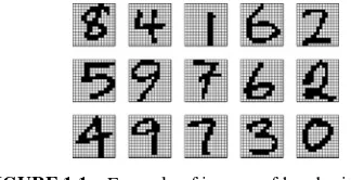
Pattern recognition is about assigning labels to objects. Objects are described by features, also called attributes. A classic example is recognition of handwritten digits for the purpose of automatic mail sorting. Figure 1.1 shows a small data sample. Each 15×15 image is one object. Its class label is the digit it represents, and the features can be extracted from the binary matrix of pixels.

1.1.1 Classes and Class Labels

Intuitively, a class contains similar objects, whereas objects from different classes are dissimilar. Some classes have a clear-cut meaning, and in the simplest case are mutually exclusive. For example, in signature verification, the signature is either genuine or forged. The true class is one of the two, regardless of what we might deduce from the observation of a particular signature. In other problems, classes might be difficult to define, for example, the classes of left-handed and right-handed people or ordered categories such as “low risk,” “medium risk,” and “high risk.”

(26)

FIGURE 1.1 Example of images of handwritten digits.

We shall assume that there arecpossible classes in the problem, labeled from𝜔₁ to𝜔_c, organized as a set of labelsΩ ={𝜔₁,…,𝜔_c}, and that each object belongs to one and only one class.

1.1.2 Features

Throughout this book we shall consider numerical features. Such are, for example, systolic blood pressure, the speed of the wind, a company’s net profit in the past 12 months, the gray-level intensity of a pixel. Real-life problems are invariably more complex than that. Features can come in the forms of categories, structures, names, types of entities, hierarchies, so on. Such nonnumerical features can be transformed into numerical ones. For example, a feature “country of origin” can be encoded as a binary vector with number of elements equal to the number of possible countries where each bit corresponds to a country. The vector will contain 1 for a specified country and zeros elsewhere. In this way one feature gives rise to a collection of related numerical features. Alternatively, we can keep just the one feature where the categories are represented by different values. Depending on the classifier model we choose, the ordering of the categories and the scaling of the values may have a positive, negative, or neutral effect on the relevance of the feature. Sometimes the methodologies for quantifying features are highly subjective and heuristic. For example, sitting an exam is a methodology to quantify a student’s learning progress. There are also unmeasurable features that we as humans can assess intuitively but can hardly explain. Examples of such features are sense of humor, intelligence, and beauty.

Once in a numerical format, the feature values for a given object are arranged as an n-dimensional vectorx=[x₁,…,x_n]T _∈_Rn_{. The real space}

Rnis called thefeature space, each axis corresponding to a feature.

(27)

BASIC CONCEPTS: CLASS, FEATURE, DATA SET 3

1.1.3 Data Set

The information needed to design a classifier is usually in the form of a labeled data setZ={z₁,…,zN},zj∈Rn. The class label ofzj is denoted byyj∈ Ω, j= 1,…,N. A typical data set is organized as a matrix ofN rows (objects, also called examples or instances) byncolumns (features), with an extra column with the class labels

◻

◼

_{Example 1.1} _{A shape–color synthetic data set}

Consider a data set with two classes, both containing a collection of the following objects:▵,,○,▴,, and

t

_{. Figure 1.2 shows an example of such a data set. The}

collections of objects for the two classes are plotted next to one another. Class𝜔₁is shaded. The features are only the shape and the color (black or white); the positioning of the objects within the two dimensions is not relevant. The data set contains 256 objects. Each object is labeled in its true class. We can code the color as 0 for white and 1 for black, and the shapes as triangle=1, square=2, and circle=3.

(28)

Based on the two features, the classes are not completely separable. It can be observed that there are mostly circles in 𝜔₁ and mostly squares in 𝜔₂. Also, the proportion of black objects in class𝜔₂is much larger. Thus, if we observe a color and a shape, we can make a decision about the class label. To evaluate the distribution of different objects in the two classes, we can count the number of appearances of each object. The distributions are as follows:

Object

▵

◦

▴

t

Class𝜔1 9 22 72 1 4 20

Class𝜔2 4 25 5 8 79 7

Decision 𝜔1 𝜔2 𝜔1 𝜔2 𝜔2 𝜔1

With the distributions obtained from the given data set, it makes sense to choose class𝜔₁if we have a circle (of any color) or a white triangle. For all other possible combinations of values, we should choose label 𝜔₂. Thus using only these two features for labeling, we will make 43 errors (16.8%).

A couple of questions spring to mind. First, if the objects are not discernible, how have they been labeled in the first place? Second, how far can we trust the estimated distributions to generalize over unseen data?

To answer the first question, we should be aware that the features supplied by the user are not expected to be perfect. Typically there is a way to determine the true class label, but the procedure may not be available, affordable, or possible at all. For example, certain medical conditions can be determined onlypost mortem. An early diagnosis inferred through pattern recognition may decide the outcome for the patient. As another example, consider classifying of expensive objects on a production line as good or defective. Suppose that an object has to be destroyed in order to determine the true label. It is desirable that the labeling is done using measurable features that do not require breaking of the object. Labeling may be too expensive, involving time and expertise which are not available. The problem then becomes a pattern recognition one, where we try to find the class label as correctly as possible from the available features.

Returning to the example in Figure 1.2, suppose that there is a third (unavailable) feature which could be, for example, the horizontal axis in the plot. This feature would have been used to label the data, but the quest is to find the best possible labeling method without it.

The second question “How far can we trust the estimated distributions to generalize over unseen data?” has inspired decades of research and will be considered later in this text.

◻

◼

_{Example 1.2 The Iris data set}

(29)

FIGURE 1.3 Iris flower specimen

recognition and has been used in thousands of publications over the years [39, 348]. This book would be incomplete without a mention of it.

The Iris data still serves as a prime example of a “well-behaved” data set. There are three balanced classes, each represented with a sample of 50 objects. The classes are species of the Iris flower (Figure 1.3): setosa, versicolor, and virginica. The four features describing an Iris flower are sepal length, sepal width, petal length, and petal width. The classes form neat elliptical clusters in the four-dimensional space. Scatter plots of the data in the spaces spanned by the six pairs of features are displayed in Figure 1.4. Class setosa is clearly distinguishable from the other two classes in all projections.

Sepal length

Sepal width

Sepal length

Petal length

Sepal length

Petal width

Sepal width

Petal length

Sepal width

Petal width

Petal length

Petal width

Setosa

Versicolor

Virginica

(30)

1.1.4 Generate Your Own Data

Trivial as it might be, sometimes you need a piece of code to generate your own data set with specified characteristics in order to test your own classification method. 1.1.4.1 The Normal Distribution The normal distribution (or also Gaussian dis-tribution) is widespread in nature and is one of the fundamental models in statistics. The one-dimensional normal distribution, denotedN(𝜇,𝜎2), is characterized by mean 𝜇∈Rand variance𝜎2∈R. Inn dimensions, the normal distribution is character-ized by an n-dimensional vector of the mean, 𝝁∈Rn, and an n×n covariance matrixΣ. The notation for an n-dimensional normally distributed random variable isx∼N(𝝁,Σ). The normal distribution is the most natural assumption reflecting the following situation: there is an “ideal prototype” (𝝁) and all the data are distorted versions of it. Small distortions are more likely to occur than large distortions, caus-ing more objects to be located in the close vicinity of the ideal prototype than far away from it. The scatter of the points around the prototype𝝁is associated with the covariance matrixΣ_i.

The probability density function (pdf) ofx∼N(𝝁,Σ) is

where|Σ|is the determinant ofΣ. For the one-dimensional case,xand𝜇are scalars, andΣreduces to the variance𝜎2. Equation 1.1 simplifies to

p(x)= _√1

◻

◼

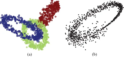
_{Example 1.3 Cloud shapes and the corresponding covariance matrices} Figure 1.5 shows four two-dimensional data sets generated from the normal distribu-tion with different covariance matrices shown underneath.

(d)

(31)

Figures 1.5a and 1.5b are generated withindependent(noninteracting) features. Therefore, the data cloud is either spherical (Figure 1.5a), or stretched along one or more coordinate axes (Figure 1.5b). Notice that for these cases the off-diagonal entries of the covariance matrix are zeros. Figures 1.5c and 1.5d represent cases where the features aredependent. The data for this example was generated using the functionsamplegaussianin Appendix 1.A.1.

In the case ofindependent featureswe can decompose then-dimensional pdf as a product ofnone-dimensional pdfs. Let𝜎_k2be the diagonal entry of the covariance matrixΣfor thek-th feature, and𝜇_kbe thek-th component of𝝁. Then

p(x)= 1 (2𝜋)n2 √|Σ|

exp{−1 2(x−𝝁)

T_Σ−1_(x₋

𝝁)

}

= n ∏

k=1 (

1 √

(2𝜋)𝜎_k exp

{

−1 2

(

xk−𝜇k 𝜎_k

)2})

. (1.3)

Thecumulative distribution functionfor a random variableX∈Rwith a normal distribution, Φ(z)=P(X≤_z), is available in tabulated form from most statistical textbooks.1

1.1.4.2 Noisy Geometric Figures Sometimes it is useful to generate your own data set of a desired shape, prevalence of the classes, overlap, and so on. An example of a challenging classification problem with five Gaussian classes is shown in Figure 1.6 along with the MATLAB code that generates and plots the data.

One possible way to generate data with specific geometric shapes is detailed below. Suppose that each of thecclasses is described by a shape, governed by parametert.

FIGURE 1.6 An example of five Gaussian classes generated using thesamplegaussian

function from Appendix 1.A.1.

1_Φ₍_z_{) can be approximated with error at most 0.005 for 0}_≤_z_≤₂_._{2 as [150]} Φ(z)=0.5+z(4.4−z)

(32)

The noise-free data is calculated fromt, and then noise is added. Lettibe the parameter for class𝜔_i, and [ai,bi] be the interval fortidescribing the shape of the class. Denote by pi the desired prevalence of class 𝜔i. Knowing that p1+⋯+pc=1, we can calculate the approximate number of samples in a data set ofN objects. LetNi be the desired number of objects from class𝜔_i. The first step is to sample uniformlyNi values fortifrom the interval [ai,bi]. Subsequently, we find the coordinatesx1,…,xn for each element oft_i. Finally, noise is added to all values. (We can use therandn MATLAB function for this purpose.) The noise could be scaled by multiplying the values by different constants for the different features. Alternatively, the noise could be scaled with the feature values or the values oft_i.

◻

◼

_{Example 1.4 Ellipses data set}

The code for producing this data set is given in Appendix 1.A.1. We used the parametric equations for two-dimensional ellipses:

x(t)=xc+acos(t)cos(𝜙)−bsin(t)sin(𝜙), y(t)=yc+acos(t)sin(𝜙)−bsin(t)cos(𝜙),

where (xc,yc) is the center of the ellipse,aandbare respectively the major and the minor semi-axes of the ellipse, and𝜙is the angle between thex-axis and the major axis. To traverse the whole ellipse, parametertvaries from 0 to 2𝜋.

Figure 1.7a shows a data set where the random noise is the same across both fea-tures and all values oft. The classes have equal proportions, with 300 points from each class. Using a single ellipse with 1000 points, Figure 1.7b demonstrates the effect of scaling the noise with the parametert. The MATLAB code is given in Appendix 1.A.1.

(a) (b)

FIGURE 1.7 (a) The three-ellipse data set; (b) one ellipse with noise variance proportional

to the parametert.

(33)

CLASSIFIER, DISCRIMINANT FUNCTIONS, CLASSIFICATION REGIONS 9

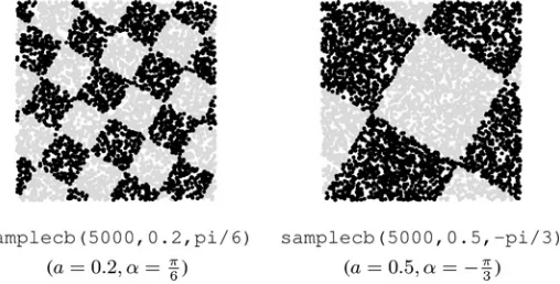
FIGURE 1.8 Rotated checker board data (100,000 points in each plot).

parameteraspecifies the side of the individual square. For example, ifa=0.5, there will be four squares in total before the rotation. Figure 1.8 shows two data sets, each containing 5,000 points, generated with different input parameters. The MATLAB functionsamplecb(N,a,alpha)in Appendix 1.A.1 generates the data.

The properties which make this data set attractive for experimental purposes are:

r

_{The two classes are perfectly separable.}

r

_{The classification regions for the same class are disjoint.}

r

_{The boundaries are not parallel to the coordinate axes.}

r

_{The classification performance will be highly dependent on the sample size.}

1.2 CLASSIFIER, DISCRIMINANT FUNCTIONS,

CLASSIFICATION REGIONS

Aclassifieris any function that will assign a class label to an objectx:

D:Rn→Ω. (1.4)

In the “canonical model of a classifier” [106],c discriminant functionsare calculated

g_i :Rn→R, i=1,…,c, (1.5)

each one yielding a score for the respective class (Figure 1.9). The objectx∈Rnis labeled to the class with the highest score. This labeling choice is called themaximum membership rule. Ties are broken randomly, meaning thatxis assigned randomly to one of the tied classes.

The discriminant functions partition the feature spaceRnintoc decision regions orclassification regionsdenoted₁,…,_c:

i= {

x||

||x∈Rn,g_i(x)= max k=1,…,c gk(x)

}

(34)

1

2

…

c Feature

vector

Maximum selector

MAX

Discriminant functions

Class label

FIGURE 1.9 Canonical model of a classifier. Ann-dimensional feature vector is passed

throughcdiscriminant functions, and the largest function output determines the class label.

The decision region for class𝜔_iis the set of points for which thei-th discriminant function has the highest score. According to the maximum membership rule, all points in decision regioniare assigned to class𝜔i. The decision regions are specified by the classifierD, or equivalently, by the discriminant functionsG. The boundaries of the decision regions are calledclassification boundariesand contain the points for which the highest discriminant functions tie. A point on the boundary can be assigned to any of the bordering classes. If a decision region_icontains data points from the labeled setZwith true class label𝜔_j,j≠i, classes𝜔_iand𝜔_jare calledoverlapping. If the classes inZcan be separated completely by a hyperplane (a point inR, a line inR2, a plane inR3), they are calledlinearly separable.

Note that overlapping classes in a given partition can be nonoverlapping if the space was partitioned in a different way. If there are no identical points with dif-ferent class labels in the data setZ, we canalwayspartition the feature space into pure classification regions. Generally, the smaller the overlapping, the better the clas-sifier. Figure 1.10 shows an example of a two-dimensional data set and two sets of classification regions. Figure 1.10a shows the regions produced by the nearest neighbor classifier, where every point is labeled as its nearest neighbor. According to these boundaries and the plotted data, the classes are nonoverlapping. However, Figure 1.10b shows the optimal classification boundary and the optimal classification regions which guarantee the minimum possible error for unseen data generated from the same distributions. According to the optimal boundary, the classes are overlap-ping. This example shows that by striving to build boundaries that give a perfect split we may over-fit the training data.

Generally,anyset of functionsg₁(x),…,g_c(x) is a set ofdiscriminant functions. It is another matter how successfully these discriminant functions separate the classes.

Let G∗₌_{_g∗

(35)

CLASSIFICATION ERROR AND CLASSIFICATION ACCURACY 11

(a) (b)

FIGURE 1.10 Classification regions obtained from two different classifiers: (a) the 1-nn boundary (nonoverlapping classes); (b) the optimal boundary (overlapping classes).

Applying the samef to all discriminant functions inG∗, we obtain an equivalent set of discriminant functions. Using the maximum membership rule,xwill be labeled to the same class by any of the equivalent sets of discriminant functions.

1.3 CLASSIFICATION ERROR AND CLASSIFICATION ACCURACY

It is important to know how well our classifier performs. Theperformance of a classifier is a compound characteristic, whose most important component is the classification accuracy. If we were able to try the classifier on all possible input objects, we would know exactly how accurate it is. Unfortunately, this is hardly a possible scenario, so an estimate of the accuracy has to be used instead.

Classification error is a characteristic dual to the classification accuracy in that the two values sum up to 1

Classification error=1−Classification accuracy.

The quantity of interest is called thegeneralization error. This is the expected error of the trained classifier on unseen data drawn from the distribution of the problem.

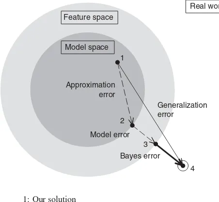
1.3.1 Where Does the Error Come From? Bias and Variance

(36)

Real world Feature space

Model space 1

2

3

4 Approximation

error

Generalization error

Model error

Bayes error

1: Our solution

2: Best possible solution with the chosen model

3: Best possible solution with the available features 4: The “real thing”

FIGURE 1.11 Composition of the generalization error.

minimum of the criterion function. If started from a different initialization point, the solution may be different. In addition to the approximation error, there may be a model error. Point 3 in the figure is the best possible solution in the given feature space. This point may not be achievable with the current classifier model. Finally, there is an irreducible part of the error, calledthe Bayes error. This error comes from insufficient representation. With the available features, two objects with the same feature values may have different class labels. Such a situation arose in Example 1.1. Thus the true generalization errorP_Gof a classifierDtrained on a given data set Zcan be decomposed as

P_G(D,Z)=P_A(Z)+P_M+P_B, (1.7)

whereP_A(Z) is the approximation error,P_Mis the model error, andP_B is the Bayes error. The first term in the equation can be thought of as variance due to using different training data or non-deterministic training algorithms. The second term,P_M, can be taken as the bias of the model from the best possible solution.

(37)

Target

Low bias, high variance

Target

High bias, low variance

FIGURE 1.12 Bias and variance.

grouped together, variance is low. Then the distance to the target will be more due to the bias. Conversely, widely scattered solutions indicate large variance, and that can account for the distance between the shot and the target.

1.3.2 Estimation of the Error

Assume that a labeled data setZ_tsof sizeN_ts×nis available for testing the accuracy of our classifier,D. The most natural way to calculate an estimate of the error is to runDon all the objects inZ_tsand find the proportion of misclassified objects, called sometimes theapparent error rate

̂

PD= N_error

N_ts . (1.8)

Dual to this characteristic is the apparent classification accuracy which is calculated by 1−_P̂

D.

To look at the error from a probabilistic point of view, we can adopt the following model. The classifier commits an error with probabilityPD on any object x∈Rn (a wrong but useful assumption). Then the number of errors has a binomial distribution with parameters (P_D,N_ts). An estimate of P_D is_P̂

D. IfNts andPD satisfy the rule of thumb:N_ts >30,_P̂

D×Nts>5, and (1−P̂D)×Nts>5, the binomial distribution can be approximated by a normal distribution. The 95% confidence interval for the error is

(38)

1.3.3 Confusion Matrices and Loss Matrices

To find out how the errors are distributed across the classes we construct aconfusion matrix using the testing data set, Z_ts. The entry aij of such a matrix denotes the number of elements fromZ_ts whose true class is𝜔_i, and which are assigned byD to class𝜔_j. The estimate of the classification accuracy can be calculated as the trace of the matrix divided by the total sum of the entries. The additional information that the confusion matrix provides iswherethe misclassifications have occurred. This is important for problems with a large number of classes where a high off-diagonal entry of the matrix might indicate a difficult two-class problem that needs to be tackled separately.

◻

◼

_{Example 1.5 Confusion matrix for the Letter data}

The Letters data set, available from the UCI Machine Learning Repository Database, contains data extracted from 20,000 black-and-white images of capital English letters. Sixteen numerical features describe each image (N=20,000,c=26,n=16). For the purpose of this illustration we used the hold-out method. The data set was randomly split into halves. One half was used for training a linear classifier, and the other half was used for testing. The labels of the testing data were matched to the labels obtained from the classifier, and the 26×26 confusion matrix was constructed. If the classifier was ideal, and all assigned and true labels were matched, the confusion matrix would be diagonal.

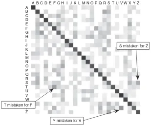
Table 1.1 shows the row in the confusion matrix corresponding to class “H.” The entries show the number of times that true “H” is mistaken for the letter in the respective column. The boldface number is the diagonal entry showing how many times “H” has been correctly recognized. Thus, from the total of 350 examples of “H” in the testing set, only 159 have been labeled correctly by the classifier. Curiously, the largest number of mistakes, 33, are for the letter “O.” Figure 1.13 visualizes the confusion matrix for the letter data set. Darker color signifies a higher value. The diagonal shows the darkest color, which indicates the high correct classification rate (over 69%). Three common misclassifications are indicated with arrows in the figure.

TABLE 1.1 The “H”-row in the Confusion Matrix for the Letter Data Set Obtained from a Linear Classifier Trained on 10,000 Points

“H” labeled as: A B C D E F G H I J K L M

Times: 1 6 1 18 0 1 2 159 0 0 30 0 1

“H” labeled as: N O P Q R S T U V W X Y Z

(39)

FIGURE 1.13 Graphical representation of the confusion matrix for the letter data set. Darker color signifies a higher value.

The errors in classification are not equally costly. To account for the different costs of mistakes, we introduce theloss matrix. We define a loss matrix with entries𝜆_{i j}

denoting the loss incurred by assigning label𝜔_i, given that the true label of the object is𝜔_j. If the classifier is “unsure” about the label, it may refuse to make a decision. An extra class called “refuse-to-decide” can be added to the set of classes. Choosing the extra class should be less costly than choosing a wrong class. For a problem withcoriginal classes and a refuse option, the loss matrix is of size (c+1)×c. Loss matrices are usually specified by the user. A zero–one loss matrix is defined as𝜆_ij=0 fori=jand𝜆_ij=1 fori≠j; that is, all errors are equally costly.

1.3.4 Training and Testing Protocols The estimate_P̂

Din Equation 1.8 is valid only for the given classifierDand the testing set from which it was calculated. It is possible to train a better classifier from different training data sampled from the distribution of the problem. What if we seek to answer the question “How well can thisclassifier modelsolve the problem?”

(40)

to build the classifier (training), and also as much as possible unseen data to test its performance (testing). However, if we use all data for training and the same data for testing, we mightovertrainthe classifier. It could learn perfectly the available data but its performance on unseen data cannot be predicted. That is why it is important to have a separate data set on which to examine the final product. The most widely used training/testing protocols can be summarized as follows [216]:

r

_{Resubstitution}_{. Design classifier}_D_on_Z_{and test it on}_Z._P̂

Dis likely optimisti-cally biased.

r

_Hold-out_{. Traditionally, split}_Z_{randomly into halves; use one half for training}

and the other half for calculating_P̂

D. Splits in other proportions are also used.

r

_{Repeated hold-out (Data shuffle)}_{. This is a version of the hold-out method where}

we doL random splits ofZinto training and testing parts and average all L estimates ofP_Dcalculated on the respective testing parts. The usual proportions are 90% for training and 10% for testing.

r

_{Cross-validation}_{. We choose an integer}_K _{(preferably a factor of}_N_{) and}

ran-domly divideZintoKsubsets of sizeN∕K. Then we use one subset to test the performance ofDtrained on the union of the remaining K−1 subsets. This procedure is repeatedKtimes choosing a different part for testing each time.

To get the final value of_P̂_D_{we average the}_K_estimates.

To reduce the effect of the single split intoKfolds, we can carry out repeated cross-validation. In anM×K-fold cross validation, the data is splitMtimes into Kfolds, and a cross-validation is performed on each such split. This procedure results inM×Kestimates of_P̂

D, whose average produces the desired estimate. A 10×10-fold cross-validation is a typical choice of such a protocol.

r

_{Leave-one-out}_{. This is the cross-validation protocol where}_K₌_N_{, that is, one}

object is left aside, the classifier is trained on the remainingN−1 objects, and the left out object is classified._P̂

Dis the proportion of theNobjects misclassified in their respective cross-validation fold.

r

_Bootstrap_{. This method is designed to correct for the optimistic bias of}

resubsti-tution. This is done by randomly sampling with replacementLsets of cardinality N from the original set Z. Approximately 37% (1∕e) of the data will not be chosen in a bootstrap replica. This part of the data is called the “out-of-bag” data. The classifier is built on the bootstrap replica and assessed on the out-of-bag data (testing data).Lsuch classifiers are trained, and the error rates on the respective testing data are averaged. Sometimes the resubstitution and the out-of-bag error rates are taken together with different weights [216].

Hold-out, repeated hold-out and cross-validation can be carried out withstratified sampling. This means that the proportions of the classes are preserved as close as possible in all folds.

(41)

growing sizes of the data sets collected in different fields of science and practice pose a new challenge. We are back to using the good old hold-out method, first because the others might be too time-consuming, and second, because the amount of data might be so excessive that small parts of it will suffice for training and testing. For example, consider a data set obtained from retail analysis, which involves hundreds of thousands of transactions. Using an estimate of the error over, say, 10,000 data points, can conveniently shrink the confidence interval and make the estimate sufficiently reliable. It is now becoming common practice to use three instead of two data sets: one for training, one forvalidation, and one for testing. As before, the testing set remains unseen during the training process. The validation data set acts as pseudo-testing. We continue the training process until the performance improvement on the training set is no longer matched by a performance improvement on the validation set. At this point the training should be stopped so as to avoid overtraining. Not all data sets are large enough to allow for a validation part to be cut out. Many of the data sets from the UCI Machine Learning Repository Database2[22], often used as benchmarks in pattern recognition and machine learning, may be unsuitable for a three-way split into training/validation/testing. The reason is that the data subsets will be too small and the estimates of the error on these subsets would be unreliable. Then stopping the training at the point suggested by the validation set might be inadequate, the estimate of the testing accuracy might be inaccurate, and the classifier might be poor because of the insufficient training data.

When multiple training and testing sessions are carried out, there is the question of which of the classifiers built during this process we should use in the end. For example, in a 10-fold cross-validation, we build 10 different classifiers using different data subsets. The above methods are only meant to give us an estimate of the accuracy of a certain model built for the problem at hand. We rely on the assumption that the classification accuracy will change smoothly with the changes in the size of the training data [99]. Therefore, if we are happy with the accuracy and its variability across different training subsets, we should finally train a our chosen classifier on the whole data set.

1.3.5 Overtraining and Peeking

Testing should be done on previouslyunseendata. All parameters should be tuned on the training data. A common mistake in classification experiments is to select a feature set using the given data, andthenrun experiments with one of the above protocols to evaluate the accuracy of that set. This problem is widespread in bioinformatics and neurosciences, aptly termed “peeking” [308, 346, 348, 370]. Using the same data is likely to lead to an optimistic bias of the error.

◻

◼

_{Example 1.6 Tuning a parameter on the testing set is wrong}

(42)

5 10 15 20 0.05

0.1 0.15

Error

Training error

5 10 15 20

0.22 0.24 0.26

Steps (Common sense → Specialism)

Error

Testing error

FIGURE 1.14 Example of overtraining: letter data set.

1000 objects from the letters data set. The remaining 19,000 objects were used for testing. A quadratic discriminant classifier (QDC) was used.3_{We vary a parameter}

r,r∈[0, 1], called the regularization parameter, which determines to what extent we sacrifice adjustment to the given data in favor of robustness. Forr=0 there is no regularization; we have more accuracy on the training data and less certainty that the classifier will perform well on unseen data. For r=1, the classifier might be less accurate on the training data but can be expected to perform at the same rate on unseen data. This dilemma can be translated into everyday language as “specific expertise” versus “common sense.” If the classifier is trained to expertly recognize a certain data set, it might have this data-specific expertise and little common sense. This will show as high testing error. Conversely, if the classifier is trained to have good common sense, even if not overly successful on the training data, we might expect it to have common sense with any data set drawn from the same distribution. In the experiment,rwas decreased for 20 steps, starting withr₀=0.4 and taking r_k₊₁ to be 0.8×rk. Figure 1.14 shows the training and the testing errors for the 20 steps.

This example is intended to demonstrate the overtraining phenomenon in the process of varying a parameter, therefore we will look at the tendencies in the error curves. While the training error decreases steadily withr, the testing error decreases to a certain point, and then increases again. This increase indicates overtraining, where the classifier becomes too much of a data-specific expert and loses common sense. A common mistake in this case is to declare that the QDC has a testing error of 21.37% (the minimum in the bottom plot). The mistake is in that thetestingset was used to find the best value ofr.

(43)

EXPERIMENTAL COMPARISON OF CLASSIFIERS 19

The problem of peeking, largely due to unawareness of its caveats, is alarmingly common in application studies on feature selection. In view of this, we discuss this issue further in Chapter 9.

1.4 EXPERIMENTAL COMPARISON OF CLASSIFIERS

There is no single “best” classifier. Classifiers applied to different problems and trained by different algorithms perform differently [107, 110, 173, 196]. Comparative studies are usually based on extensive experiments using a number of simulated and real data sets. When talking about experiment design, I cannot refrain from quoting again and again a masterpiece of advice by George Nagy titledCandide’s practical principles of experimental pattern recognition[287] (Just a note—this is a joke! DO NOT DO THIS!)

r

_{Comparison of classification accuracies.}_{Comparisons against algorithms} pro-posed by others are distasteful and should be avoided. When this is not possible, the following Theorem of Ethical Data Selection may prove useful.

r

_Theorem._{There exists a set of data for which a candidate algorithm is superior} to any given rival algorithm. This set may be constructed by omitting from the test set any pattern which is misclassified by the candidate algorithm.

r

_{Replication of experiments.}_{Since pattern recognition is a mature discipline, the} replication of experiments on new data by independent research groups, a fetish in the physical and biological sciences, is unnecessary. Concentrate instead on the accumulation of novel, universally applicable algorithms.

r

_{Casey’s caution.}_{Do not ever make your experimental data available to others;} someone may find an obvious solution that you missed.

Albeit meant to be satirical, the above principles are surprisingly widespread and closely followed! Speaking seriously now, the rest of this section gives some practical tips and recommendations.

A point raised by Duin [110] is that the performance of a classifier depends upon the expertise and thewillingnessof the designer. There is not much to be done for classifiers with fixed structures and training procedures (called “automatic” classifiers in [110]). For classifiers with many training parameters however, we can make them work or fail. Keeping in mind that there are no rules defining a fair comparison of classifiers, here are a few (non-Candide’s) guidelines:

1. Pick the training procedures in advance and keep them fixed during training. When publishing, give enough detail so that the experiment is reproducible by other researchers.

(44)

TABLE 1.2 The 2×2 Relationship Table with Counts

D2correct (1) D2wrong (0)

D₁correct (1) N₁₁ N₁₀

D1wrong (0) N01 N00

Total,N11+N10+N01+N00=Nts

a totally different classifier, then it is not clear who deserves the credit—the modification or the original model itself.

3. Make sure that all the information about the data is utilized by all classifiers to the largest extent possible. For example, a clever initialization of a method can make it favorite among a group of equivalent but randomly initialized methods. 4. Make sure that the testing set has not been seen at any stage of the training. 5. If possible, give also the complexity of the classifier: training and running

times, memory requirements, and so on.

1.4.1 Two Trained Classifiers and a Fixed Testing Set

Suppose that we have two trained classifiers which have been run on the same testing data giving testing accuracies of 98% and 96%, respectively. Can we claim that the first classifier is significantly better than the second one?

McNemar test.The testing results for two classifiersD1andD2on a testing set with

N_tsobjects can be organized as shown in Table 1.2. We consider two output values: 0 for incorrect classification and 1 for correct classification. ThusN_pqis the number of objects in the testing set with outputpfrom the first classifier and outputqfrom the second classifier,p,q∈{0, 1}.

The null hypothesisH₀is that there is no difference between the accuracies of the two classifiers. If the null hypothesis is correct, then the expected counts for both off-diagonal entries in Table 1.2 are1

2(N01+N10). The discrepancy between the expected and the observed counts is measured by the following statistic:

s=

(

|N₀₁−N10|−1)2

N₀₁+N₁₀ , (1.10)

which is approximately distributed as𝜒2with 1 degree of freedom. The “−1” in the numerator is a continuity correction [99]. The simplest way to carry out the test is to calculates and compare it with the tabulated𝜒2 value for, say, level of significance4_𝛼₌₀_._{05. If}_s_>₃_._{841, we reject the null hypothesis and accept that the}

4_The_{level of significance}_{of a statistical test is the probability of rejecting}_H

(45)

EXPERIMENTAL COMPARISON OF CLASSIFIERS 21

two classifiers have significantly different accuracies. A MATLAB function for this test, calledmcnemar, is given in Appendix 1.A.2.

◻

◼

_{Example 1.7 A comparison on the Iris data}

We took the first two features of the Iris data (Example 1.2) and classes “versicolor” and “virginica.” The data was split into 50% training and 50% testing parts. The testing data is plotted in Figure 1.15. The linear and the quadratic discriminant classifiers

Sepal length

Sepal width

linear

quadratic

versicolor virginica

FIGURE 1.15 Testing data from the Iris data set and the decision boundaries of the linear and the quadratic discriminant classifiers.

(LDC and QDC, both detailed later) were trained on the training data. Their decision boundaries are plotted in Figure 1.15.

The confusion matrices of the two classifiers are as follows:

LDC QDC

Versicolor Virginica Versicolor Virginica

Versicolor 20 5 Versicolor 20 5

Virginica 8 17 Virginica 14 11

Taking LDC to be classifier 1 and QDC, classifier 2, the values in Table 1.2 are as follows:N₁₁=31,N₁₀=0,N₀₁=6, andN₀₀=13. The difference is due to the six virginica objects in the “loop.” These are correctly labeled by QDC and mislabeled by LDC. From Equation 1.10,

s= (|0−6|−1)

2

0+6 =

25

6 ≈4.1667. (1.11)

Combining Pattern Classifiers, 2nd Edition

Combining

Pattern Classifiers

Methods and Algorithms,

Second Edition

COMBINING PATTERN

CLASSIFIERS

Methods and Algorithms

Second Edition

CONTENTS

PREFACE

ACKNOWLEDGEMENTS

1

FUNDAMENTALS OF PATTERN

RECOGNITION

◻

◼

t

▵

◦

▴

t

◻

◼

◻

◼

◻

◼

r

r

r

r

…

◻

◼

r

r

r

r

r

r

◻

◼

r

r

r

r

◻

◼