NEW EMPIRICAL FORMULAE OF UNDERTOW VELOCITY ON MIXED AND GRAVEL BEACHES | antoniadis | JOURNAL OF COASTAL DEVELOPMENT 5155 11306 1 PB

(1)

158

Original paper

NEW EMPIRICAL FORMULAE OF UNDERTOW VELOCITY ON

MIXED AND GRAVEL BEACHES

Christos antoniadis

External Research Fellow in Port Engineering in Civil Engineering Department of Democritus University of Thrace, Xanthi, 67100, Greece

Received : February 3, 2013; Accepted: February 27, 2013

ABSTRACT

This paper reports a series of 3-dimensional physical model tests to measure cross-shore current data, generated by oblique wave attack, along gravel and mixed beaches with a uniform slope and a trench. Coastal managers and coastal engineers are beginning to give attention to gravel and mixed beaches due to the fact that they are two of the most effective natural sea defences.There is a need, from a scientific and coastal management perspective to have a deeper understanding of how gravel and mixed beaches operate.The studies described in this paper aim to investigate the behaviour of the undertow velocity on mixed and gravel beaches. Existing formulae have been used to predict the experimental results and new equations for predicting the undertow velocity under these conditions are proposed.

The new empirical formulae predict time- and depth-averaged undertow and are based on a nonlinear regression of a modification of the Grasmeijer’s and Ruessink’s model where the zones where divided based on the related distance of the point of interest and the breaking point. Verification with large-scale experiments showed that the new formulae predicted well the undertow velocities on mixed and gravel beach with trench and uniform slope.

Keywords: gravel, mixed beach, wave-induced currents, trench, wave breaking, undertow

*

Correspondence: Phone:+30- 6979708081; Fax: +30- 2541062939; E-mail: cantoniadis79@hotmail.com

I

NTRODUCTION

As the oblique waves break to the shoreline two mean currents are generated flowing parallel (long-shore currents) and straight normal (cross-shore currents) to the coast. These two mean currents can be considered as components of a continuum flow field from which the resulting wave-induced mean current structure is illustrated in Fig. 1(Svendsen and Lorenz, 1989). These nearshore currents in combination with the stirring action of the waves are important for the sediment transport and therefore are significant factors in morphological changes. Consequently, they are of great importance for managers of coastal areas, coastal engineers and marine geologistics (Visser, 1991).

Cross-shore currents are related to the mass compensation under breaking waves and

they are not constant over depth (Coastal Engineering Manual, 2003). The main characteristic of the cross-shore current is the existence of the two-dimensional circulation in the surf zone known as “undertow current”, which flows in the seawards direction from the shoreline. This current is directed offshore on the bottom, balanced with the onshore flow of water carried by the breaking waves. Closer to the water surface the resulting current is in the onshore direction. The undertow current may be relatively strong, being almost 8% to 10% of the wave celerity ( ) near the bottom.

(2)

159

trough, and the hydrostatic excess pressure caused by the local mean water level gradient (setup), which becomes predominant below wave trough level (Briand and Kamphuis, (Briand and Kamphuis, 1993; Svendsen, 1984a and Deigaardet al., 1991). Svendsen and Buhr Hansen (1988).

To extend our understanding within the coastal environment a 3-dimensional physical

model (see

Fig. 2,

Fig. 3,

Table 1 and Table 2) was used to examine wave breaking formulae for obliquely incident waves on mixed and gravel beaches (Antoniadis, 2009).

M

ATERIALS AND

M

ETHODS

The Experiment

The experiments were carried out in the three-dimensional wave basin located at Franzius-Institute (Marienwerder), Hannover University. in the middle of the wave basin. It was open to the side from which the generated waves were approaching. The beach model was oriented in such a way that waves, generated by the wave paddle, were always approaching it with an angle of 150 (Fig.2). Beach bathymetry consisted of a uniform slope beach (straight-line parallel contour) and a trench (curved contour) with a width of 2m, as shown in Fg.3. The location and the dimensions of the trench in the physical model would not have any significant impact in the profile changes of the beach with the uniform slope.

(3)

160

curved beach section and the other two at the straight beach section, for all three space directions Vx, Vy and Vz. These sections are shown as lines in Fig.3. Velocities Vx and Vy were considered positive when heading towards the positive direction of x and y axes (Fig.3), measurements that was taken was satisfactory. Current velocity measurements were carried out at various levels along the z direction. At each level, the current velocity measurements were taken over a period of 60 seconds. Observations for regular waves started at the surface and deepened with a constant 5cm integral until the maximum point was reached. The maximum point was the point at which the ADV could take logical measurements, usually that was between 5 and 10cm above the bed level. The deepest point of measurement was 35cm below water surface.

The same procedure was followed for random waves but with a 10cm integral. The deepest point of measurement for random waves was 30cm below the water surface. This procedure allowed an estimate of the vertical structure of the time-averaged velocity and a more accurate determination of the averaged current velocities. The depth-averaged current velocity V was determined as:

Data Analysis measurement points were before the breaking point but close enough the undertow current to be observed. The undertow was represented (in Appendix A) by the seaward direction of the currents. Furthermore, at the trench, the seaward direction of the currents could represent rip currents, especially at Test 1 and

Test 2 where the highest wave conditions of the experiment occurred.

Rip currents are usually confused with the undertow. As the waves move to the shoreline produces setup. Because of the inclination of the water level, the setup water is essentially piled up against the shoreline in an unstable condition. If this unstable condition exists along a barred coast or along some of the steeper coasts, the setup produces seaward flowing currents that are rather narrow and that create circulation cells within the surf zone. These narrow currents are called rip currents.

When wind and waves push water towards the shore, the previous backwash is often pushed sideways by the oncoming waves. This water streams along the shoreline until it finds an exit back to the sea. The resulting rip current is usually narrow and located in a trench. In general, while a common misconception is that a rip occurring under the water, instead of on top — an undertow — is strong enough to drag people under the surface of the water; the current is actually strongest at the surface. In some areas, rip currents will persist during low- to moderate- energy wave conditions and then during high-energy wave conditions the rips will lose their definition and undertow will be primary mode of seaward return of water from unstable condition of setup.

(4)

161

presented at

Fig. 4 to

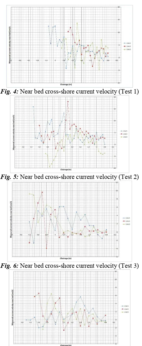
Fig. 13. In the y-direction, positive indicates seaward where negative indicates shoreward.

The cross-shore current velocity was expected to be very small, close to zero, near

the bed. However, in

Fig. 4 to

Fig. 13, velocities were not always zero or small. It was expected currents to have higher values close to the breaking point. However, during the tests, currents had relatively high values (for both shoreward and seaward directions) even before the breaking point. The shoreward currents had maximum value near to 5cm/s. The near bed cross-shore currents have shown an oscillating direction, from seaward to shoreward and from shoreward to seaward, along the cross-shore section of the beach.

Lara et al. (2002), showed how the undertow behaves over a highly permeable bed. They conducted an experimental study in a laboratory, showing the mean flow characteristics over impermeable and permeable beds. Their study discussed the differences between water surface envelopes and undertow for these cases. They showed that the effect of a permeable bed (D50=19 and 39 mm) on the undertow is a change of the velocity profile, with the magnitude of undertow close to the seafloor reduced. This effect was more important in decreasing water depth and it was reduced for decreasing gravel size.

(5)

162

at the tests with gravel beach. By comparing the magnitude of velocities between the gravel and mixed bed, it can be seen that the velocities were higher at the gravel bed where the D50 was also the highest. This is in agreement with the observation of Lara et al. (2002).

Nevertheless, the increase and even the change of direction of the velocities near the bed, especially in the gravel bed, can be due to the mechanism of bed-generated turbulence. Lara et al. (2002) stated that the gravel bed-generated turbulence characteristics depend on the gravel size and increasing gravel size results in an increase in the velocity gradient, which is the principal mechanism for the generation of larger-scale turbulence over the gravel bed. This mechanism of bed-generated turbulence has been noticed by Buffin-Bélanger

et al. (2000) and Shvidchenko et al. (2001) over gravel bed rivers resulting in Reynolds stresses that have different signs, revealing different vortex orientation (Lara et al., 2002).

In the surf zone, the turbulence can be related to the type of breaking because partly or even the whole mechanism for the generation of turbulence is induced to the breaking process. The characteristics of turbulence structure and undertow are different in spilling and plunging breakers. Turbulent kinetic energy is transported seaward under the spilling breaker. This is different from the plunging breaker where turbulent kinetic energy is transported landward (Ting and Kirby, 1994).

R

ESULTS AND

D

ISCUSSION

Results

Comparison with other existing methods

In this section, a comparison is given with other existing formulations that calculate the time-averaged and depth-averaged undertow. Various authors have presented models for predicting cross-shore currents, especially undertow.

Kuriyama and Nakatsukasa (2000) developed a one-dimensional model which predicts the time- and depth- averaged undertow velocities. The model was calibrated with field data obtained over longshore bars at Hazaki Oceanographical Research Station

(HORS) and it predicted well the undertow over the longshore bars.

Grasmeijer and Ruessink (2003) presented a hydrodynamic model that can predict also the time-averaged cross-shore currents (undertow) in a parametric and probabilistic mode. The model was calibrated with laboratory and field experiments and it predicted well the undertow. Furthermore, Tajima and Madsen (2006) developed a near-shore current model based on Tajima and Madsen’s (2002, 2003) wave and surface roller models. There was a generally good agreement of predicted the undertow velocity profiles by using the model.

Pedrozo-Acuna et al. (2006) presented an estimation of the value of the undertow velocity from a Boussinesq model by explicitly allowing for the higher velocity in the roller region of a breaking wave front (e.g. Madsen et al., 1997). The value of undertow Uo was

The experimental data was compared with the models of Kuriyama and Nakatsukasa (2000) and Grasmeijer and Ruessink (2003). The model of Grasmeijer and Ruessink (2003) was used in parametric mode as its authors stated that it would give the same accuracy with a computationally quicker approach than the probabilistic mode. The calculation procedures of both models are presented in Appendix B and C.

(6)

163

mass fluxes in a different way. The model of Kuriyama and Nakatsukasa (2000) did not include the angle of incidence; however, in the comparison with the experimental results, it was included. At the model of Grasmeijer and Ruessink (2003), the procedure of calculating the roller area was not described. However, in the comparison with the experimental results, the roller area was presented and calculated twice based on the following two equations: Engelund (1981) made a simple dynamic model of a hydraulic jump, which is based on the depth-integrated horizontal momentum equation and gives the local thickness of the surface roller. Engelund assumed that the boundary between surface roller and the water below is a straight line. Using an analogy between the velocity distribution in separated diffuser flow and in the hydraulic jump, it was argued that the angle θ between this boundary and the horizontal is about 100. With accuracy within a few per cent the roller area obtained by the model of Engelund (1981) can be calculated as

(3)

Duncan (1981) has made measurements of rollers in waves that have been generated by a towel hydrofoil. Svendsen (1984b) approximated these results with the relation

(4)

(7)

164

generally underestimated by the models (except for gravel beach-regular waves).

The model of Kuriyama and Nakatsukasa (2000) with the inclusion of the angle of incidence, had better correlation than the other models, with uniform slope for regular wave conditions (with both mixed and gravel beach) and with trench for random wave conditions (with both mixed and gravel beach). In general, the correlations of this model (Kuriyama and Nakatsukasa, 2000) with the measured data were poor because it was initially developed and calibrated with the undertow velocities measured over longshore bars and it mainly has been applied on barred beaches.

The model of Grasmeijer and Ruessink (2003) in relation with the equation of Svendsen (1984b), had better correlation with the other models, with trench for regular wave conditions (with both mixed and gravel beach) and with uniform slope for random wave agreement with the measurements. The discrepancies may be caused by the use of linear wave theory to compute the mean mass transport associated with the organised wave motion in the model. As for this model (Grasmeijer and Ruessink, 2003) and the model of Kuriyama and Nakatsukasa (2000), it is needless to say that the predictive performance of the 2D model is poor for cases where 3D circulations are important.

New empirical equations

Based on a non-linear regression analysis, empirical relations have been generated in order to predict much more accurate the experimental results. These empirical relations are based on the results of the model Grasmeijer and Ruessink (2003). The non-linear regression has been fitted to the data and the proposed fits are shown by the following equations:

Regular Wave Conditions

For gravel beach (trench):

(5)

For gravel beach (uniform slope):

(6) For mixed beach (trench):

(7) For mixed beach (uniform slope):

(8)

Random Wave Conditions

(8)

165

(9) For gravel beach (uniform slope):

(10)

For mixed beach (trench):

(11)

For mixed beach (uniform slope):

(12)

where

U (cm/s) is the depth- and time-averaged undertow velocity with positive values for seaward direction,

uGB (cm/s) is the value of the output of the model of Grasmeijer and Ruessink (2003), X is the dimensional parameter which is equal

to , and

A is the dimensional parameter which is equal to point and the point of interest

Db (m) is the distance from the point, where the local water depth is equal to the still water level, to the breaking point

Di (m) is the distance from the point, where the local water depth is equal to the still water level, to the point of interest

The breaking depth for regular waves was calculated (Rattanapitikon and Shibayama, 2006) by

(13a)

(13b) and for random waves (Goda 1970,1985) by

(14) where A= a coefficient (=0.12)

The breaking point is defined as the maximum wave height admissible for a given water depth (Torrini and Allsop, 1999).

(9)

166

tests, with the proposal equations (Eq. (5) to

Eq. (12)) are shown in

Fig.23 to

Fig.30 (the positive values represent the undertow velocities). In these figures, Eq. (5) to Eq. (12) show better agreement with the experimental data compared with the models of Kuriyama and Nakatsukasa (2000) and Grasmeijer and Ruessink (2003).

Discussion

The analysis of the cross-shore currents in both gravel and mixed beaches focused on the behaviour of the undertow and especially its behaviour near the bed. The undertow was observed in both trench and uniform slope for both types of beach. However, near the bed, the trench had higher values of undertow flow compare to the uniform slope beach and also had higher values with mixed beach compare to gravel beach. In addition, the velocities were higher at the gravel bed where the D50 was also the highest which was in agreement with the observation of Lara et al. (2002).

The cross-shore currents near the bed for both gravel and mixed beaches showed no reduction of their values and also showed an oscillated direction, from seaward to shoreward and from shoreward to seaward, along the cross-shore section of the beach. This behaviour including the case where the value of the cross-shore current velocity increased instead of being decreased can be caused from the permeability of the beach and also the mechanism of the bed-generated turbulence (Buffin-Bélanger et al., 2000 and Shvidchenko

et al., 2001). This behaviour influenced the cross-shore sediment transport at the bed and it is more noticeable at gravel beach due to its higher permeability compare with mixed beach. The new empirical formulae estimated the undertow velocity by dividing the cross-section area based on the location of the point of interest and the breaking point compared to the local water depth. The new formulae estimated the undertow velocity more accurately than the the models of Kuriyama and Nakatsukasa (2000) and Grasmeijer and Ruessink (2003).

C

ONCLUSIONS

This paper investigated the behaviour of the undertow velocity on mixed and gravel beaches with uniform slope and a trench. New empirical formulae, based on the model of Grasmeijer modification of the Grasmeijer’s and Ruessink’s model where the zones where divided based on the related distance of the point of interest and the breaking point.

(10)

167

A

CKNOWLEDGEMENTS

The author would like to acknowledge the assistance and support provided by staff of Cardiff University and by staff of Franzius-Institute (Marienwerder) of University of Hannover for the completion of the physical model tests.

R

EFERENCES

Antoniadis C., 2009.Wave-induced currents and sediment transport on gravel and mixed beaches. Ph.D. Thesis. Cardiff University, UK, 591 pp.

Briand, M.-H., G., and Kamphuis J.W., 1993. Waves and currents on natural beaches: a quasi 3D numerical model. J. of Coast.

Coastal Engineering Manual, 2003. Surf zone hydrodynamics. EM 1110-2-100, Part II, Chapter 4, US Army Corps. of Engineers, 40pp.

Dally, W. R., and Dean, R. G. 1984. Suspended Sediment Transport and Beach Profile Evolution. J. of Wat., Por., Coast., and Oc. Eng., 110 (1), 15-33.

Deigaard, R., Justesen, P., Fredsoe, J., 1991. Modelling of undertow by a one-equation turbulence model. Coastal Engineering, 15, 431-458.

Duncan, J.H., 1981. An Experimental Investigation of Breaking Waves Produced by a Towed Hydrofoil.p. 331-38. In:Proc. R. Soc. Lond. A, 377, 8 July 1981.RSP.

Dyhr-Nielsen, M., and Sorensen, T., 1970. Some Sand Transport Phenomena on Coasts with Bars.p.1993-2004.In:

Proceedings of the 12th Coastal

Engineering Conference, American

Society of Civil Engineers.

Engelund, 1981. F. Engelund, A simple theory of weak hydraulic jumps.p.29-31. In:

Progress Report No. 54, Institute of

Hydrodynamics and Hydraulic Engineering, ISVA, Technical University Denmark, 1981.

Grasmeijer, B.T., and uessink, B.G., 2003. Modelling of waves and currents in the nearshore parametric vs. Probabilistic approach. J. of Coast. Eng., 49, 185-207. Goda, Y., 1970. A synthesis of breaker indices.

Trans. JSCE, 2, 227-230.

Goda, Y., 1983. A unified nonlinearity parameter of water waves. Report of Port Harbour Res. Inst., 22 (3), 3-30. Goda, Y., 1985. Random Seas and Design of

Maritime Structures. University of Tokyo Press., ISBN 0-86008-369-1, Tokyo, 464pp.

Hansen, J. B., and Svendsen, I. A., 1984. A Theoretical and Experimental Study of Undertow.p.2246-2262.In: Proceedings barred beach.p.247-260.In:Proc. 25th Coastal Eng. Conf., ASCE.

Kuriyama, Y., and Ozaki, Y., 1996. Wave height and fraction of breaking waves on a bar-trough beach – field measurements at HORS and modelling. Report Port Harbour Res. Inst., 35 (1), 1-38.

Kuriyama, Y., and Nakatsukasa, T., 2000. A one-dimensional model for undertow and longshore current on a barred beach.

Journal of Coastal Engineering, 40, 39-58.

Lara, J.L., Losada, I.J., Cowen, E.A., 2002. Large-scale turbulence structures over an immobile gravel-bed inside the surf zone. p. 1050-1061. In: Smith, J.M. (Ed.), 28th International Conference on Coastal Engineering, WS, Cardiff, UK. Madsen, P.A., Sørensen, O.R., Schaffer, H.A.,

1997. Surf zone dynamics simulated by a Boussinesq type model: Part I. Model description and crossshore motion of regular waves. Coast. Eng., 32, 255– 287.

(11)

168

beaches. Journal of Coastal Engineering, 53, 335-347.

Rattanapitikon, W., and Shibayama, T., 2006. Breaking wave formulas for breaking depth and orbital to phase velocity ratio.

Coast. Eng. J., 48 (4), 395-416.

Seyama, A., and Kimura, A., 1988. The measured properties of irregular wave breaking and wave height change after breaking on the slope.p.419-432.In:Proc. 21st Coastal Eng. Conf., ASCE.

Shvidchenko, A.B., Pender, G., Hoey, T.B., 2001. Critical shear stress for incipient motion of sand/gravel streambeds. Water Resources Research, 37, 2273-2284. Stive, M. J. F., and Wind, H. F. 1986.

Cross-shore Mean Flow in the Surf Zone.

Coastal Engineering, 10 (4), 325-340. Svendsen, I.A., 1984a. Mass flux and undertow

in a surf zone. Coastal Engineering, 8, Undertow and the Boundary Layer Flow on a Beach. J. of Geoph. Res., 92 (C11), Velocities in combined undertow and longshore currents. Coast. Eng., 13, 55-79.

Tajima, Y., and Madsen, O. S., 2002. Shoaling, breaking and broken wave characteristics.p.222-234.In:Proc., 28th Int. Conf. on Coastal Engineering, ASCE, Reston, Va..

Tajima, Y., and Madsen, O. S., 2003. Modeling near-shore waves and surface rollers. In:Proc., 2nd Int. Conf. on Asian and

Pacific Coasts _CD-ROM_, World

Scientific, Singapore, ISBN 981-238-558-4.

Tajima, Y., and Madsen, O. S., 2006. Modeling near-shore waves, surface rollers, and undertow velocity profiles. Journal of Waterway, Port, Coastal, and Ocean Engineering, 132(6), 429-438.

Ting, F.C.K., and Kirby, J.T., 1994. Observation of undertow and turbulence in a laboratory surf zone. Coastal Engineering, 24, 51-80.

Torrini, L., and Allsop, N.W.H., 1999. Goda’s breaking prediction method- A discussion note on how this should be applied. HR Report, IT 473, Wallingford, U.K.

Visser, P. J., 1991. Laboratory Measurements of Uniform Longshore Currents. Coast. Eng.,15(5),563-593.

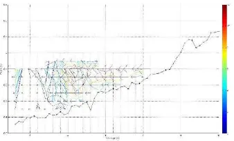
Appendix A

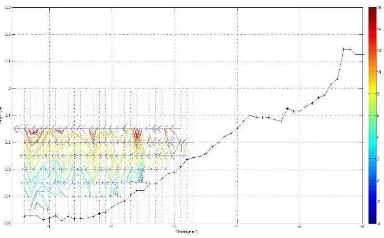
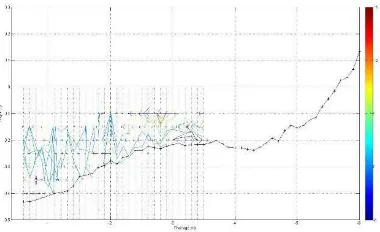
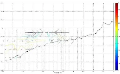
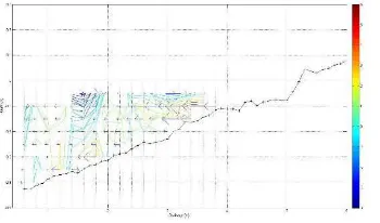
Observation of the cross-shore currents, of each individual test and line, during the experiment

(12)

169

Fig. A.2:2D presentation of the time-averaged currents (cm/s) for Test 1- Line 2

(13)

170

(14)

171

(15)

172

(16)

173

(17)

174

(18)

175

Appendix B

The undertow model of Kuriyama and Nakatsukasa (2000)

The time- and depth-averaged undertow velocity of an individual wave Vind is estimated

with the volume flux due to the organised wave motion Qw and that due to the surface roller Qr.

(19)

176 consideration for the wave nonlinearity. With the parameter Π expressing nonlinearity of an individual wave and experimental data shown by Goda (1983), the relationship between ζrms and H was obtained; the parameter Π and the relationship obtained are expressed by:

(B.4)

(B.5)

In the estimation of Qr, the volume flux due to the roller is obtained from

(B.6)

where Ar is the area of the roller. The area of the surface roller is estimated on the basis of the assumptions mentioned below.

The area of the surface roller is basically assumed to be proportional to the square of the wave height. The area Ar1 is estimated with a dimensionless coefficient CA from

(B.7)

where CA is given by

(B.8)

where ξb is the surf similarity parameter at the wave breaking position and is estimated by

(B.9)

where tanβ is the bed slope, L1/3,0 is the offshore wavelength corresponding to the significant wave period and H1/3,b is the significant wave height at the wave-breaking position and is estimated by:

For random waves (Kuriyama, 1996):

(B.10)

For regular waves (Seyama and Kimura, 1988):

(20)

177

where Hb is the wave breaking height, hb is the wave breaking depth and L0 is the wavelength in deep water. Cbr is a dimensionless coefficient with a range from 0.7 to 1.2.

where Wr is the energy of the roller having the distribution of the time-averaged velocity above the wave trough level, Ew is the energy of the organized wave motion (=ρgH2/8), Cg is the group velocity, ρ is the sea water density, T is the wave period, H is the wave height, h is

the water depth, and B is a dimensionless coefficient determining the amount of energy dissipation. Kuriyama and Ozaki (1996) investigated the coefficient B with the experimental data of Seyama and Kimura (1988), and proposed the following formula:

(B.15) be the area of the surface roller.

Appendix C

The undertow model of Grasmeijer and Ruessink (2003)

The time- and depth-averaged undertow velocity is derived from the mass flux due to the wave motion (Qw) and the mass flux due to the surface roller (Qr).

(C.1)

where htrough= h- H/2

where h is the water depth and H is the wave height. For random waves H is represented by Hrms.

Using linear theory, Qw is computed as

(C.2)

where E is the wave energy (=cosθρgH2/8) for obliquely waves, θ is the angle of incidence, ρ is the density of the water and c is the wave phase speed.

The roller distribution Qr is computed as (Svendsen, 1984a)

(C.3)

where A is the roller area, T is the wave period and Er is the roller energy density and is estimated by

(21)

178

Figures

Fig. 1: Schematic diagram of the vertical profile of the mean cross-shore and longshore current in the nearshore

Fig. 2: Position of the beach model

(22)

179

Fig. 4: Near bed cross-shore current velocity (Test 1)

(23)

180

Fig. 10:Near bed cross-shore current velocity (Test 7)

(24)

181

Fig. 14:Estimated vs. Measured undertow velocity (Regular waves/gravel beach - trench)

(25)

182

Fig. 16:Estimated vs. Measured undertow velocity (Regular waves/mixed beach- trench)

Fig. 17:Estimated vs. Measured undertow velocity (Regular waves/mixed beach- uniform slope)

Fig. 18:Estimated vs. Measured undertow velocity (Random waves/gravel beach- trench)

(26)

183

Fig. 20:Estimated vs. Measured undertow velocity (Random waves/mixed beach- trench)

Fig. 21:Estimated vs. Measured undertow velocity (Random waves/mixed beach- uniform slope)

Fig. 22:Schematisation of the components of A and X

(27)

184

Fig.24:Estimated vs. Measured undertow velocity (Regular waves/gravel beach – uniform slope)

Fig.25:Estimated vs. Measured undertow velocity (Regular waves/Mixed Beach - trench)

Fig.26:Estimated vs. Measured undertow velocity (Regular waves/Mixed Beach – uniform slope)

(28)

185

Fig.28:Estimated vs. Measured undertow velocity (Random waves/gravel beach – uniform slope)

Fig.29:Estimated vs. Measured undertow velocity (Random waves/Mixed Beach - trench)

Fig.30:Estimated vs. Measured undertow velocity (Random waves/Mixed Beach – uniform slope)

Tables

Table 1.The different particle sizes of the sediments Type of Beach D5

(29)

186

Test 3-G 8.6 cm 2 sec Test 9-M 11 cm 2.3 sec

Test 4-G 9.2 cm 3 sec Test 10-M 11.7 cm 3.1 sec

Test 7-M 8.6 cm 2 sec