T H E J O U R N A L O F H U M A N R E S O U R C E S • 46 • 3
The Phantom Gender Difference in
the College Wage Premium
William H. J. Hubbard
A B S T R A C T
A growing literature seeks to explain why so many more women than men now attend college. A commonly cited stylized fact is that the college wage premium is, and has been, higher for women than for men. After identify-ing and correctidentify-ing a bias in estimates of college wage premiums, I find that there has been essentially no gender difference in the college wage premium for at least a decade. A similar pattern appears in quantile wage regressions and for advanced degree wage premiums.
I. Introduction
Today in the United States, more women than men attend and gradu-ate from college, a dramatic change from recent decades. This development has spawned a growing literature that attempts to identify its causes. See Chiappori, Iyigun, and Weiss (2009); Goldin, Katz, and Kuziemko (2006); DiPrete and Buch-mann (2006); Dougherty (2005). Perhaps the most prominent stylized fact in this literature has been that the college wage premium for women is higher than the college wage premium for men (and has been for at least 40 years).1
This stylized fact has framed the discussion in this literature: a higher return to education for women explains why more women than men attend college today, but it leaves unanswered why more men attended college in the past (since the college wage premium was higher for women in the past as well). Hence, some scholars
1. The college wage premium is generally defined, and I define it here, as the difference in log wages between college graduates and high school graduates with no college education.
William H.J. Hubbard is the Kauffman Legal Research Fellow at the University of Chicago Law School and a Ph.D. Candidate in the University of Chicago Economics Department. He is grateful for com-ments from Gary Becker, Pierre-Andre Chiappori, Jonathan Hall, Devon Haskell, Ethan Lieber, Lee Lockwood, Kevin Murphy, Derek Neal, Emily Oster, Genevieve Pham-Kanter, Mark Phillips, Jesse Sha-piro, Hugo Sonnenschein, Andrew Zuppann, and participants in the Workshop in Applications of Eco-nomics at the University of Chicago. The data used in this article can be obtained beginning six months after publication through three years hence from William H. J. Hubbard, University of Chicago Law School, 1111 E. 60th Street, Chicago, IL 60637, or by email at whubbard@uchicago.edu. [Submitted December 2009; accepted July 2010]
have looked to factors that prevented women in the past from exploiting the higher college wage premium for women. Goldin, Katz, and Kuziemko (2006) point to past barriers to women’s education and careers; as these barriers fell, the gender differ-ence in the college wage premium became decisive: “According to most estimates, the college (log or percentage) wage premium is actually higher for women than men, and it has been for some time. . . . As the labor force participation of women has begun to resemble men’s, women have responded to the monetary returns.” Analogously, Chiappori, Iyigun, and Weiss (2009) combine an exogenous fall in the time required for housework and “the higher labor-market returnto schooling for women” to explain the relative rise in women’s college attainment.
But what if this stylized fact, the starting point for these arguments, is wrong? I will argue that the college wage premium for women isnotlarger for women than men, and we must revisit our accounts of the dramatic rise in women’s college attainment relative to men. Most recent estimates rely on Current Population Survey (CPS) wage data that are “topcoded” or censored at a maximum value. Topcoding biases estimates of the college wage premium downward for males relative to fe-males, and the magnitude of this bias has grown over time. Once I account for this bias, I find no gender difference in the college wage premium in recent years.
This paper proceeds as follows. Section II briefly discusses recent estimates of the college wage premiums for men and women. None of these estimates adequately accounts for the bias caused by censoring. Section III presents facts on topcoding and shows how topcoding can bias estimates of the college wage premium. Section IV describes the data set I use in my estimates. In Section V, I reestimate college wage premiums for men and women using CPS data after accounting for topcodes, and show that the college wage premium is not larger for women than for men, at least in recent years. Section VI concludes.
II. Existing Estimates
The near-consensus in the literature has been that college wage pre-miums are higher for women than for men, and have been since at least the 1960s. This claim rests primarily on analysis of the March CPS data series, which, for all years since 1963, provides a continuous series of annual, cross-sectional, nationally representative data on education, earnings, and hours worked.2 Chiappori, Iyigun, and Weiss (2009) look at white workers age 25–54 during years 1975–2004 and conclude that “women receive a higher increase in wages than men when they acquire college or advanced degrees.” Using CPS data for 1963 to 2001, DiPrete and Buchmann (2006) report an earnings gap of about 0.1 to 0.2 log points among 30–34 year old full-time/full-year (FTFY) white workers for the entire study period. Charles and Luoh (2003) use CPS data from 1961–97. Comparing those with at least two years of college to those with no college, they find that the wage premium
570 The Journal of Human Resources
for women is consistently about 0.2 log points higher than for men. Card and DiNardo (2002) use CPS data for years 1975–99 and report college wage premiums for women that are greater than or equal to those of men for all years.
Some studies use data sources other than the CPS. Dougherty (2005) runs wage regressions on years of schooling using National Longitudinal Survey of Youth 1979 (NLSY79) data and finds higher wage premiums for women throughout the period 1988–2000. He also cites more than 20 other studies that use data sources other than the CPS and find higher “returns to schooling” for women than men. None of these studies, however, looks at data from 1990 or later. Pen˜a (2007) disagrees with these findings, but offers only evidence from outside the United States to support the claim that the college wage premium is higher for men.
III. Topcoding and Topcode Bias
Wage and salary earnings data (“wage income” or “wages”) in CPS public use files have been topcoded since 1967. From 1967–80, the topcode was 50,000; from 1981–83, it was 75,000; from 1984–94, it was 99,999; from 1995– 2001, it was 150,000; and since 2002, it has been 200,000.3 These are nominal values; all income data, including topcodes, reported in the CPS are in current year dollars.
Topcoding is a widely recognized issue for CPS data. See, for example, Katz and Murphy (1992); Card and DiNardo (2002); Autor, Katz, and Kearney (2005); Di-Prete and Buchmann (2006); Mulligan and Rubinstein (2008); Hirsh and McPherson (2008); Larrimore et al. (2008). I have found no prior study, however, that has identified and examined the biasing effect of topcodes on the college wage premium. (Although they do not discuss bias due to topcoding, Katz and Murphy (1992) do adjust topcoded wages before calculating college wage premiums for the years 1963– 87. Card and DiNardo (2002) note the presence of topcodes and suggest adjusting them by a factor of 1.4, although their results described above do not make this adjustment.) Instead, some prior work has attempted to address the presence of topcodes by recensoring wage data at maximum values that are more consistent across time. For example, DiPrete and Buchmann (2006) recensor the 1963–2001 CPS wage data at topcodes that are linearly smoothed over time (and always below 124,000); Card and DiNardo (2002) recensor all observations after 1994 at 100,000. This type of correction should avoid spurious jumps in estimated wages in years when topcodes change.
Recensoring, however, greatly increases the number of observations that are sub-ject to censoring in recent years. Recensoring of wage observations has lead to larger
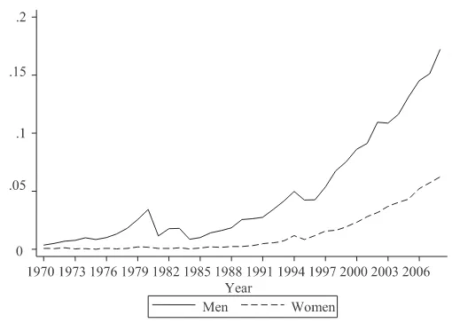
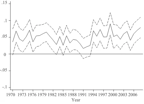
Figure 1
Fraction of All Wage Observations Subject to Censoring, by Sex
and larger numbers of censored wage observations. Figure 1 shows the dramatic rise in the share of observations in my sample (described in Section IV) subject to topcoding or recensoring at 100,000.
Crucially, for estimates of the college wage premium, the increase over time in the censoring of wage observations is not benign. First, the overwhelming majority of topcoded or recensored observations in any year are college-educated individuals. Because of this, using topcoded data without accounting for censoring will bias college wage premium estimates downward. Second, the great majority of topcoded or recensored observations are male. Thus, we would expect topcoding bias to dis-proportionately depress the college wage premium for males. Together, these facts suggest that topcoding and recensoring have increasingly biased estimates of the relative college wage premiums of women and men.
IV. Data and Construction of Samples
To estimate college wage premiums after accounting for topcodes, I use the IPUMS CPS data series for 1970–2008.4I construct a sample that is fairly representative of the samples used in the literature: I include white, non-Hispanic, adult civilians who were age 18 to 65 at the time of survey and who worked the previous year as private or government employees for a wage or salary. I exclude
572 The Journal of Human Resources
observations with negative CPS sample weights.5 I further restrict the sample to workers with 1–40 years of potential experience, as defined below. I limit the sample to full-time, full-year (FTFY) workers, where FTFY is defined as 35 or more hours per week and 50 or more weeks per year.
I focus on FTFY workers for two reasons. First, the 1994 CPS redesign was intended to increase the measured labor force participation of workers (believed to be mostly women) who in previous survey formats were being recorded as not in the labor force. Given that FTFY workers are the subset of workers who are least likely to be affected by recategorizing workers on the margin of labor force partic-ipation, I reduce any potential spurious trend generated by the 1994 survey redesign. Second, studies that have attempted to independently verify the accuracy of CPS wage data find that FTFY wage data appear to be very accurately reported, while wages for part-time, part-year workers appear to be substantially underreported. See Roemer (2000, 2002).
The coding of educational variables in the CPS data changed between 1990 and 1991. For 1970–90, the education variable is the number of whole and partial years of education completed (topcoded at 18). For 1991–2008, the education variable is coded as intervalled years of schooling for observations with less than a high school degree, and as the highest degree obtained for those with at least a high school degree, with a separate category for some college with no college degree. To ensure maximum consistency across time, I generate the following educational category recodes:
I define Dropout as anyone with fewer than 12 years of schooling completed (1970–90) or less than a high school diploma or General Education Development (GED) certificate (1991–2008); High School Graduateas anyone with exactly 12 years of schooling completed (1970–90) or exactly a high school diploma or GED certificate (1991–2008);Some Collegeas anyone with more than 12 and fewer than 16 years of schooling completed (1970–90) or categorized as “Associate Degree” or “Some College, No Degree” by the CPS (1991–2008);Bachelor’s Degreeas 16 or 17 years of schooling completed (1970–90)6or categorized as “Bachelor’s De-gree” by the CPS (1991–2008); andAdvanced Degreeas 18 or more years of school-ing completed (1970–2008) or categorized as “Masters,” “Professional,” or “Doc-torate” degree holder by the CPS (1991–2008). I defineCollege Graduate as any observation that I have defined as either Bachelor’s Degree or Advanced Degree above.
I also generate a “Years of School” variable. As noted above, the CPS reports years of schooling only until 1990. For 1991–2008, I impute years of completed schooling as follows: I divide the sample into demographic cells based on sex and educational category. For each demographic cell, I compute the mean years of schooling during the period 1988–90. These values, rounded down to the nearest integer, are the years of schooling used for observations in the same demographic categories for 1991–2008. With this measure of years of school, I generate potential experience asAGE – YEARS OF SCHOOL – 7.
I deflate all wage values using the Personal Consumption Expenditures (PCE) price index to 1982 dollars, and drop all observations with annual wages less than $3,484, or one-half minimum wage in 1982. For a 52-week year, this is equivalent to the $67/week threshold used in Katz and Murphy (1992) and Mulligan and Ru-binstein (2008).7 Finally, I also exclude observations flagged as containing “allo-cated” (imputed) values for education or the amount or source of wage and salary income. No results are sensitive to the inclusion or exclusion of either type of im-puted data. Table 1 provides descriptive statistics for the sample.
V. Results
I calculate college wage premiums by sex using alternate specifica-tions, each designed to account for topcoding of wage data. First, I run ordinary least squares (OLS) regressions in which topcoded wage values are adjusted to eliminate bias from censoring. Second, I deploy the Tobit model for censored re-gression. Third, I use median regressions, which are not sensitive to the values of upper-tail wages. Regardless of the method used, I find no female advantage in the college wage premium in recent years. I then examine separately the premiums associated with bachelor’s degrees and advanced degrees.
A. OLS Regression Estimates
My specification is fairly standard in the literature. I run a set of yearly regressions of log wages on a dummy for female sex, a dummy for college completion, an interaction between college completion and female sex, and a set of other controls (all of which are interacted with female sex):
ln(y)⳱␣ⳭFemⳭ␥EducⳭ␦(Fem•Educ)ⳭXⳭε
(1) i i i i i i
For my initial OLS regressions, yi is annual wage income andEduciis a dummy for college graduate. The vectorXiincludes potential experience, potential experience squared, and Census region dummies, all of them interacted with the dummy for female sex. The difference between the male and female college wage premium is the coefficient␦on the female/college interaction term.
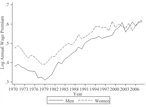
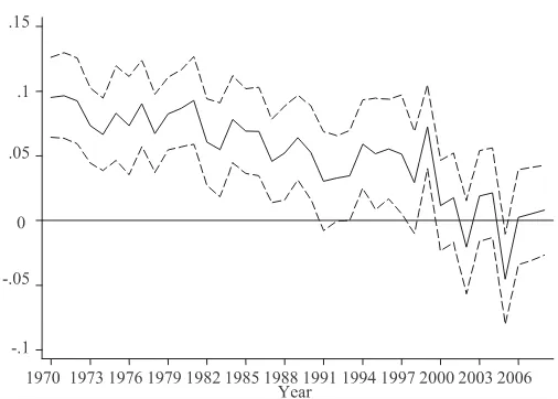
Figure 2 shows the estimates of the college wage premiums from an OLS log wage regression when wages are recensored at 100,000. This generates the familiar conclusion that the college wage premium for women has been consistently higher than the premium for men. As we see from Figure 3, the gender difference is sta-tistically significant in nearly all years, and appears to be growing in recent years.
As noted above, the problem with these estimates is that censoring wages at a topcode or censoring point Twill bias downward the coefficients of variables that tend to raise wages above . Because the true values of topcoded wage observationsT are not available, my approach is to replace topcoded log wage observations with their expected value; in other words, I choose an “adjustment factor”Asuch that I
574
The
Journal
of
Human
Resources
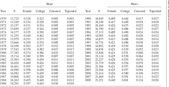
Table 1
Descriptive Statistics for Sample of March CPS Cross-Sections 1970–2008
Share Share
Year N Female College Censored Topcoded Year N Female College Censored Topcoded
1970 13,725 0.328 0.322 0.003 0.003 1990 18,849 0.409 0.444 0.017 0.017 1971 13,249 0.334 0.328 0.003 0.003 1991 18,248 0.417 0.449 0.018 0.018 1972 13,157 0.331 0.334 0.005 0.005 1992 18,160 0.424 0.473 0.022 0.022 1973 13,699 0.327 0.344 0.005 0.005 1993 16,790 0.412 0.486 0.027 0.027 1974 14,377 0.335 0.350 0.007 0.007 1994 17,313 0.409 0.490 0.034 0.034 1975 11,255 0.349 0.362 0.005 0.005 1995 14,905 0.416 0.492 0.028 0.012 1976 13,979 0.351 0.373 0.007 0.007 1996 14,855 0.413 0.488 0.030 0.014 1977 13,666 0.350 0.374 0.009 0.009 1997 14,734 0.421 0.496 0.038 0.015 1978 14,100 0.362 0.377 0.012 0.012 1998 14,802 0.419 0.510 0.046 0.020 1979 17,542 0.370 0.382 0.017 0.017 1999 14,838 0.421 0.519 0.052 0.023 1980 17,383 0.374 0.386 0.022 0.022 2000 13,849 0.421 0.531 0.060 0.026 1981 15,714 0.380 0.399 0.007 0.007 2001 23,114 0.425 0.539 0.064 0.029 1982 15,303 0.390 0.430 0.011 0.011 2002 22,227 0.428 0.553 0.076 0.017 1983 16,026 0.400 0.426 0.011 0.011 2003 21,719 0.426 0.554 0.078 0.016 1984 16,461 0.395 0.427 0.005 0.005 2004 21,366 0.421 0.557 0.084 0.018 1985 16,989 0.398 0.430 0.006 0.006 2005 21,568 0.425 0.557 0.094 0.019 1986 16,982 0.397 0.439 0.009 0.009 2006 21,414 0.424 0.580 0.106 0.023 1987 19,006 0.402 0.428 0.010 0.010 2007 21,460 0.431 0.591 0.111 0.023 1988 18,363 0.405 0.440 0.012 0.012 2008 21,251 0.440 0.601 0.124 0.026 1989 19,291 0.397 0.443 0.016 0.016
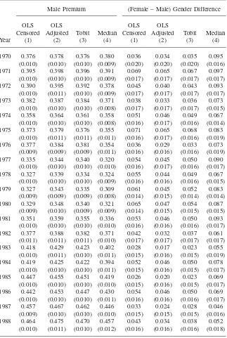
Table 2
Estimates of College Wage Premium (with Standard Errors), March CPS 1970–2008
Male Premium (Female – Male) Gender Difference
OLS
1970 0.376 0.378 0.376 0.380 0.036 0.034 0.035 0.095 (0.010) (0.010) (0.010) (0.009) (0.020) (0.020) (0.020) (0.016) 1971 0.395 0.398 0.396 0.391 0.069 0.065 0.067 0.097
(0.010) (0.010) (0.010) (0.009) (0.017) (0.017) (0.017) (0.017) 1972 0.390 0.395 0.392 0.378 0.045 0.040 0.043 0.093
(0.010) (0.011) (0.010) (0.009) (0.017) (0.017) (0.017) (0.017) 1973 0.382 0.387 0.384 0.371 0.038 0.033 0.036 0.073
(0.010) (0.010) (0.010) (0.008) (0.017) (0.017) (0.017) (0.015) 1974 0.358 0.364 0.361 0.358 0.051 0.046 0.049 0.067
(0.010) (0.010) (0.010) (0.008) (0.016) (0.017) (0.016) (0.014) 1975 0.373 0.379 0.376 0.355 0.071 0.065 0.068 0.083
(0.010) (0.011) (0.011) (0.011) (0.016) (0.017) (0.016) (0.019) 1976 0.377 0.384 0.381 0.354 0.036 0.029 0.033 0.073
(0.009) (0.009) (0.009) (0.011) (0.016) (0.016) (0.016) (0.019) 1977 0.335 0.344 0.340 0.320 0.054 0.045 0.050 0.090
(0.010) (0.010) (0.010) (0.010) (0.016) (0.017) (0.016) (0.017) 1978 0.327 0.339 0.334 0.324 0.055 0.044 0.049 0.067
(0.010) (0.010) (0.010) (0.009) (0.016) (0.016) (0.016) (0.015) 1979 0.327 0.343 0.335 0.309 0.061 0.045 0.052 0.083
(0.009) (0.009) (0.009) (0.008) (0.014) (0.015) (0.014) (0.014) 1980 0.329 0.348 0.340 0.321 0.065 0.047 0.054 0.087
(0.009) (0.010) (0.009) (0.009) (0.014) (0.015) (0.015) (0.015) 1981 0.351 0.359 0.355 0.336 0.053 0.046 0.050 0.093
(0.010) (0.010) (0.010) (0.010) (0.016) (0.016) (0.016) (0.017) 1982 0.377 0.388 0.382 0.371 0.042 0.032 0.037 0.061
(0.011) (0.011) (0.011) (0.010) (0.017) (0.017) (0.017) (0.017) 1983 0.418 0.429 0.423 0.402 0.028 0.017 0.023 0.055
(0.010) (0.011) (0.010) (0.011) (0.015) (0.016) (0.015) (0.019) 1984 0.419 0.425 0.422 0.394 0.052 0.046 0.050 0.078
(0.010) (0.010) (0.010) (0.011) (0.015) (0.016) (0.015) (0.017) 1985 0.447 0.455 0.451 0.419 0.026 0.020 0.023 0.069
(0.010) (0.010) (0.010) (0.010) (0.015) (0.016) (0.015) (0.017) 1986 0.442 0.453 0.447 0.430 0.054 0.046 0.050 0.069
(0.010) (0.010) (0.010) (0.011) (0.016) (0.016) (0.016) (0.017) 1987 0.457 0.467 0.462 0.446 0.033 0.024 0.028 0.046
(0.009) (0.010) (0.010) (0.010) (0.015) (0.015) (0.015) (0.016) 1988 0.464 0.475 0.470 0.457 0.043 0.034 0.038 0.052
(0.010) (0.011) (0.010) (0.012) (0.016) (0.016) (0.016) (0.018)
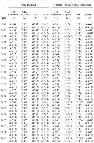
576 The Journal of Human Resources
Table 2(continued)
Male Premium (Female – Male) Gender Difference
OLS
1989 0.493 0.511 0.502 0.480 0.041 0.026 0.033 0.064 (0.010) (0.010) (0.010) (0.010) (0.015) (0.015) (0.015) (0.017) 1990 0.488 0.506 0.497 0.471 0.031 0.015 0.022 0.053
(0.010) (0.010) (0.010) (0.012) (0.015) (0.016) (0.015) ⳮ0.018
1991 0.518 0.540 0.529 0.504 0.016 ⳮ0.002 0.007 0.030
(0.010) (0.011) (0.011) (0.012) (0.015) (0.016) (0.016) (0.020) 1992 0.511 0.536 0.524 0.514 0.022 0.001 0.011 0.033
(0.010) (0.011) (0.011) (0.011) (0.016) (0.016) (0.016) (0.017) 1993 0.528 0.556 0.542 0.524 0.025 0.002 0.013 0.035
(0.011) (0.012) (0.011) (0.011) (0.016) (0.017) (0.016) (0.017) 1994 0.517 0.554 0.537 0.527 0.069 0.041 0.053 0.059
(0.011) (0.012) (0.012) (0.011) (0.017) (0.018) (0.017) (0.017) 1995 0.531 0.567 0.559 0.537 0.053 0.021 0.029 0.051
(0.012) (0.013) (0.012) (0.014) (0.017) (0.018) (0.018) (0.022) 1996 0.510 0.547 0.538 0.525 0.073 0.043 0.050 0.055
(0.011) (0.012) (0.012) (0.013) (0.017) (0.018) (0.018) (0.020) 1997 0.528 0.570 0.560 0.533 0.051 0.020 0.026 0.051
(0.011) (0.013) (0.012) (0.015) (0.017) (0.018) (0.018) (0.023) 1998 0.520 0.576 0.563 0.536 0.051 0.004 0.015 0.029
(0.011) (0.012) (0.012) (0.013) (0.017) (0.018) (0.018) (0.020) 1999 0.521 0.585 0.569 0.541 0.090 0.039 0.052 0.073
(0.011) (0.013) (0.012) (0.011) (0.017) (0.018) (0.018) (0.017) 2000 0.527 0.597 0.581 0.570 0.052 ⳮ0.001 0.011 0.012
(0.012) (0.014) (0.013) (0.011) (0.018) (0.020) (0.020) (0.018) 2001 0.542 0.617 0.600 0.582 0.057 0.000 0.013 0.018
(0.010) (0.011) (0.011) (0.011) (0.015) (0.016) (0.016) (0.018) 2002 0.543 0.624 0.613 0.608 0.044 ⳮ0.015 ⳮ0.007 ⳮ0.021
(0.010) (0.012) (0.011) (0.012) (0.015) (0.017) (0.017) (0.018) 2003 0.510 0.590 0.580 0.559 0.060 0.003 0.011 0.019
(0.010) (0.012) (0.012) (0.012) (0.016) (0.017) (0.017) (0.018) 2004 0.520 0.611 0.599 0.583 0.067 ⳮ0.004 0.006 0.021
(0.010) (0.012) (0.012) (0.011) (0.016) (0.018) (0.018) (0.018) 2005 0.530 0.635 0.621 0.611 0.041 ⳮ0.037 ⳮ0.026 ⳮ0.045
(0.010) (0.012) (0.011) (0.011) (0.016) (0.017) (0.017) (0.018) 2006 0.522 0.633 0.618 0.589 0.060 ⳮ0.019 ⳮ0.008 0.002
(0.010) (0.012) (0.012) (0.012) (0.016) (0.018) (0.017) (0.019) 2007 0.522 0.630 0.615 0.610 0.071 ⳮ0.002 0.007 0.005
(0.010) (0.012) (0.012) (0.012) (0.015) (0.018) (0.017) (0.018) 2008 0.526 0.655 0.638 0.612 0.079 ⳮ0.014 ⳮ0.002 0.008
Figure 2
College Wage Premium, OLS Regressions, Recensored Wages
Figure 3
Gender Difference in the Premium, Recensored OLS Regressions, with 95 Percent Confidence Interval Bands
can replace topcoded wage observations (observations wherey⳱T) with new values
i
(yi⳱AT) where the log of the adjusted wage is equal to the expected value of the log of the true (unobserved) wage (ln(AT)⳱E
[
ln(yi)yiT]
).578 The Journal of Human Resources
To do this, I employ the common assumption that upper-tail wages are Pareto dis-tributed. Given a Pareto distribution with minimum valuem and the Pareto index parameter , the parameterk k uniquely determines the adjustment factorA and vice versa. If wagesyiare Pareto distributed, then for any topcode value ,T
1
Thus, my task is to estimatek by year and sex. I construct the likelihood function for a censored Pareto distribution
where there are N observations, of which the first n observations are topcoded at .
T
Maximizing log likelihood yields the following estimate for :k
Nⳮn
ˆk⳱
(4) N
ln(y)Ⳮnln(T)ⳮNln(m)
兺
j⳱nⳭ1 jThe only unquantified term in Equation 4 is m. Rather than impose an a priori value form, I take advantage of the fact that the adjustment factor —and thereforeA —is known for each sex in recent years. With this information, I derive an estimate k
ofm, which I then use in Equation 4 to estimatekˆ for all years. Since 1995, each topcoded wage observation in the CPS public-use data has been replaced with the mean wages of all topcoded observations in the same sex-by-race-by-FTFY-status demographic cell (in other words, for each year and sex during 1995–2008, the CPS data provide E
[
yiyiⱖT]
). For each sex, I calculate the average ratio of these ex-pected values to the topcodes; call this (sex-specific) ratio .R8Again using the Pareto distribution, I derive a value fork directly from the ratio of topcoded values to the topcode:R k⳱
(5)
Rⳮ1
I then calibrate m for each sex such that the maximum likelihood estimate ˆk matches the k derived directly from the 1995–2008 CPS data.9 Armed with this estimate of m, I then use the estimator fork given in Equation 4 to generate ad-justment factors for each sex and year in the sample. Finally, I recensor 1995–2008 wage observations at their topcodes and multiply all topcoded wage observations
8. The values forRare 1.835 for men and 1.884 for women.
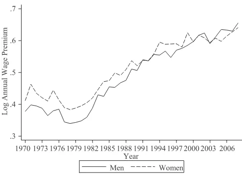
Figure 4
College Wage Premium, OLS Regressions, Adjusted Wages
for 1967–2008 by their year- and sex-specific adjustment factors before taking logs of all wage values.10
When I reestimate college wage premiums using adjusted wages, a very different picture emerges. See Figures 4 and 5.11I find little or no gender difference in the college wage premium since about 1990.
B. Tobit Regression Estimates
An alternate, and indeed simpler, way to correct for topcoding is to employ the Tobit censored regression model. This model treatsyiin Equation 1, annual wage income, as a latent variable, whose observed values are censored at an upper limit equal to the topcode value for the relevant year. This specification yields results almost iden-tical to estimates based on adjusted wages. See Figures 6 and 7. There is essentially no significant gender difference in the college wage premium since about 1990.
C. Quantile Regression Estimates
I next run quantile (median) regressions, using the same set of regressors. Figures 8 and 9 present the results of the quantile regressions. Importantly, these results are insensitive to the presence of topcodes or corrections for topcoding. In these
580 The Journal of Human Resources
Figure 5
Gender Difference in the Premium, Adjusted OLS Regressions, with 95 Percent Confidence Interval Bands
Figure 6
College Wage Premium, Tobit Regressions with Censoring at Topcode
mates, the female-male difference is larger in earlier years, but the difference narrows and then vanishes by 2000.12
Figure 7
Gender Difference in the Premium, Tobit Regressions, with 95 Percent Confidence Interval Bands
Figure 8
College Wage Premium, Quantile Regressions
D. The Advanced Degree Wage Premium
582 The Journal of Human Resources
Figure 9
Gender Difference in the Premium, Quantile Regressions, with 95 Percent Confidence Interval Bands
whose highest degree is a bachelor’s and those with advanced degrees. Such a distinction may have seemed unnecessary, because those studies that looked sepa-rately at bachelor’s and advanced degree holders have found the same pattern for each group as for all college graduates—a persistent difference in the premium favoring women. See Chiappori, Iyigun, and Weiss (2009); Card and DiNardo (2002).
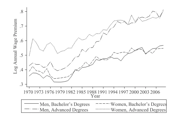
Once I account for topcoding, however, a different picture emerges. To examine advanced degrees and bachelor’s degrees separately, I use the specification in Equa-tion 1 with one change:Educiis now a vector with separate dummies for bachelor’s degree only and advanced degree. I adjust topcoded wages as described above and run OLS regressions with adjusted log wages. I find that the advanced degree wage premium for women far exceeded the advanced degree wage premium for men through the 1970s and 1980s; since then, the men’s and women’s premiums have converged. The bachelor’s degree wage premiums for men and women, however, have never differed by much. See Figures 10 and 11.13Thus, it appears that the past gender difference in the “college” wage premium was largely the product of the gender difference in theadvanced degreewage premium.
Figure 10
College Wage Premium, Adjusted OLS Regressions, by Degree Type
E. Sensitivity Analysis
In addition to the alternate estimation methods presented above, I perform further robustness checks on my methodology. First, in the spirit of Katz and Murphy (1992), I estimate college wage premiums nonparametrically by dividing the uni-verse of observations into demographic cells, and then computing the college wage premium on a cell-by-cell basis. For each cell, I compute the mean wage among high school graduates and the mean wage among college graduates; the college wage premium is the log of the ratio of these averages. I combine these cell-specific college wage premiums to estimate a yearly college wage premium for each sex. In these fixed-weight estimates, higher college wage premiums for women disappear once topcoded wage observations are adjusted.
Second, I execute fixed-weight estimates after redefining the college wage pre-mium as the log ratio of themediancollege wage to themedianhigh school wage. This yields a “fixed-weight median” estimate; the results are nearly identical to the median regression results presented above. Third, I replicate the results of several papers described in Section II. After correcting for recensoring and topcoding, I find that their results are consistent with the results I report above. All these results are presented in detail in a Web Appendix.14
584 The Journal of Human Resources
Panel A: Advanced Degree Premium
Panel B: Bachelor’s Degree Premium
Figure 11
Gender Differences, Adjusted OLS Regressions, with 95 Percent Confidence Interval Bands
VI. Conclusion
over time, and there has been no female advantage in the college wage premium for at least a decade.
This fact only deepens the puzzle of why more women now attend college than men. Women’s college attendance has overtaken men’s, even as the college wage premium for women hasfallen relative to the premium for men. This suggests that other forces, such as the nonmarket benefits of college education or the (nonpecu-niary) costs of attending college, are driving relative changes in college attendance of men and women. Indeed, current work already has begun to consider some of the nonmarket benefits to college, including its effects on marriage and divorce (Iyigun and Walsh 2007; Chiappori, Iyigun, and Weiss 2009; DiPrete and Buchmann 2006). That women may have lower (nonpecuniary) costs of attending college is a promising explanation as well. See Becker, Hubbard, and Murphy (2010); Goldin, Katz, and Kuziemko (2006); Buchmann and DiPrete (2006).
References
Autor, David H., Lawrence F. Katz, and Melissa S. Kearney. 2005. “Residual Wage Inequality: The Role of Composition and Prices.” Working Paper 11628, National Bureau of Economic Research.
Becker, Gary S., William H.J. Hubbard, and Kevin M. Murphy. 2010. “Explaining the Worldwide Boom in Higher Education of Women.”Journal of Human Capital4(3):203– 241.
Bollinger, Christopher R., and Amitabh Chandra. 2005. “Iatrogenic Specification Error: A Cautionary Tale of Cleaning Data.”Journal of Labor Economics23(2):235–57. Buchmann, Claudia, and Thomas A. DiPrete. 2006. “The Growing Female Advantage in
College Completion: The Role of Family Background and Academic Achievement.”
American Sociological Review71(4):515–41.
Card, David, and John E. DiNardo. 2002. “Skill-Biased Technological Change and Rising Wage Inequality: Some Problems and Puzzles.”Journal of Labor Economics20(4):733– 83.
Charles, Kerwin Kofi, and Ming-Ching Luoh. 2003. “Gender Differences in Completed Schooling.”Review of Economics and Statistics85(3):559–77.
Chiappori, Pierre-Andre, Murat Iyigun, and Yoram Weiss. 2009. “Investment in Schooling and the Marriage Market.”American Economic Review99(5):1689–1713.
DiPrete, Thomas A., and Claudia Buchmann. 2006. “Gender-Specific Trends in the Value of Education and the Emerging Gender Gap in College Completion.”Demography43(1):1– 24.
Dougherty, Christopher. 2005. “Why Are the Returns to Schooling Higher for Women than for Men?”Journal of Human Resources40(4):969–88.
Goldin, Claudia, Laurence F. Katz, and Ilyana Kuziemko. 2006. “The Homecoming of American College Women: The Reversal of the College Gender Gap.”Journal of Economic Perspectives20(4):133–56.
Hirsch, Barry T., and David A. Macpherson. 2008.Union Membership and Earnings Data Book: Compilations from the Current Population Survey. Washington, D.C.: Bureau of National Affairs.
Iyigun, Murat, and Randall P. Walsh. 2007. “Building the Family Nest: Premarital Investments, Marriage Markets, and Spousal Allocations.”Review of Economic Studies
586 The Journal of Human Resources
Katz, Lawrence F., and Kevin M. Murphy. 1992. “Changes in Relative Wages, 1963–1987: Supply and Demand Factors.”Quarterly Journal of Economics107(1):35–78.
Larrimore, Jeff, Richard V. Burkhauser, Shuaizhang Feng, and Laura Zayatz. 2008. “Consistent Cell Means for Topcoded Incomes in the Public Use March CPS (1976– 2007).”Journal of Economic and Social Measurement33(2–3):89–128.
Mulligan, Casey B., and Yona Rubinstein. 2008. “Selection, Investment, and Women’s Relative Wages over Time.”Quarterly Journal of Economics123(3):1061–1110. Pen˜a, Ximena. 2007. “Assortative Matching and the Education Gap.” Borradores de
Economia 427, Banco de la Republica de Colombia.
Roemer, Marc I. 2000. “Assessing the Quality of the March Current Population Survey and the Survey of Income and Program Participation Income Estimates, 1990–1996.” Available online at http://www.census.gov/hhes/www/income/publications/assess1.pdf. ———. 2002. “Using Administrative Earnings Records to Assess Wage Data Quality in the