Directory UMM :Data Elmu:jurnal:M:Multinational Financial Management:

(1)

10 (2000) 367 – 395

On the distribution and conditional

heteroscedasticity in Taiwan stock prices

Bing-Huei Lin

a,

_{*, Shih-Kuo Yeh}

b

a_{Department of Business Administration,}_{National Taiwan Uni}

6ersity of Science and Technology,

43 Keelung Road,Sec. 4,Taipei 106, Taiwan,ROC

b_{Department of Finance,}_{National Kaohsiung First Uni}

6ersity of Science and Technology,

1 Uni6ersity Road,Yuanchau,Kaohsiung, Taiwan,ROC

Received 15 July 1999; accepted 18 February 2000

Abstract

This paper studies the distribution and conditional heteroscedasticity in stock returns on the Taiwan stock market. Apart from the normal distribution, in order to explain the leptokurtosis and skewness observed in the stock return distribution, we also examine the Student-t, the Poisson – normal, and the mixed-normal distributions, which are essentially a mixture of normal distributions, as conditional distributions in the stock return process. We also use the ARMA (1,1) model to adjust the serial correlation, and adopt the GJR – gener-alized autoregressive conditional heteroscedasticity (GARCH (1,1)) model to account for the conditional heterscedasticity in the return process. The empirical results show that the mixed – normal – GARCH model is the most probable specification for Taiwan stock returns. The results also show that skewness seems to be diversifiable through portfolio. Thus the normal – GARCH or the Student-t– GARCH model which involves symmetric conditional distribution may be a reasonable model to describe the stock portfolio return process1_.

Keywords:Generalized autoregressive conditional heteroscedasticity (GARCH); Jump-diffusion process; Leptokurtosis

www.elsevier.com/locate/econbase

* Corresponding author. Tel.: +886-2-27376748; fax:+886-2-27376744. E-mail address:lin@ba.ntust.edu.tw (B.-H. Lin).

1_{JEL classification: G10; G12; G15.}

(2)

B.-H.Lin,S.-K.Yeh/J.of Multi.Fin.Manag.10 (2000) 367 – 395 368

1. Introduction

(3)

Third, the stock return might be a stationary process, such as a stable Paretian

distribution proposed by Mandelbrot (1963, 1967) and Fama (1965), Student’s t

distribution proposed by Blattberg and Gonedes (1974) and Bollerslev (1987), or a generalized exponential distribution proposed by Nelson (1991). The stock return distributions under the above stationary processes all have thicker tails than that of the normal distribution. However, these symmetric distributions are unable to account for the skewness observed in the empirical data.

The Student-t distribution is actually a continuous mixture of normal

distribu-tions where the variance is a random variable. Blattberg and Gonedes (1974) prove that if the variance of the normal follows an inverted gamma distribution then the

resulting (posterior) distribution is the Student-t. Alternatively, the discrete mixture

of normal distributions model has more economic meanings. In fact, financial theory predicts that changes in the investment and financial decision variables, such as financial and operating leverage of firms will result in adjustment to the expected return and standard deviation parameters of the distribution of a stock’s return. Moreover, there are also information signal scenarios concerning the disclosure of a firm’s earnings that lead to parameter shifts. Seasonal announcements result in return observations with higher variance during the disclosure period than during the non-announcement periods. In addition, other firm-specific information or market-wide information will also change the parameters of the distribution of the stock’s return. After examining daily returns of 30 Dow Jones stocks, Kon (1984) concluded that the discrete mixture of normal distributions model has substantially

more descriptive validity than the symmetric Student-t model.

Ball and Torous (1983) also derive and provide evidence consistent with a mixture of two normal distributions model resulting from a Bernoulli jump process to describe information arrivals which will result in changes in parameters of the distribution of a stock’s return. If stochastic jumps are modeled by means of a Poisson distribution, the resulting distribution is a discrete mixture of an infinite number of normal distributions. Ball and Torous (1985), Akgiray and Booth (1988), and Jorion (1988) all provide evidence for the Poisson – normal distribution model.

Obviously, both the GARCH specification and the jump process (either the Bernoulli jump or the Poisson jumps) can explain the leptokurtic behavior of the series. Since the statistical and economic motivations for GARCH effects and jumps are quite different, we choose a model specification that can account for the two components simultaneously. In the return process under the mixed model, after a jump has taken place, volatility will be high, but gradually it will return to normal values when a new equilibrium is reached. If we did not include the GARCH model, the large volatility following a jump would mistakenly be taken for additional jumps causing the jump intensity parameter to be overestimated.

(4)

the assumption of stochastic volatility. Duan (1995) developed a GARCH option pricing model. Cox and Ross (1976), Merton (1976) and Ahn and Thompson (1988) priced options assuming discontinuous jump processes for underlying assets. It is intuitively clear that, if jumps are present, the classical model may severely overestimate the effectiveness of short-term hedging strategies based on dynamic portfolio adjustment. Similarly, the prices of out-of-the-money options that are close to maturity will be underestimated if jumps are present that are not taken into account. Not only option prices are sensitive to jumps but also, as noted by Amin (1993), the optimal early-exercise decision for American options alters significantly when jumps are present.

In empirical studies, Pagan and Schwert (1990), Day and Lewis (1992), and Kim and Kon (1994) studied various models with conditional heteroscedasticity for stock price dynamics. Bollerslev (1987), Nelson (1991), and Kim and Kon (1994) also examined GARCH models without assumption of conditional normality for stock returns. Jarrow and Rosenfeld (1984), Ball and Torous (1985), and Akgiray and Booth (1986) all found evidence indicating the presence of jumps in the stock price process. While Jorion (1988) combined the ARCH (1) model and the jump-diffusion process, conducted tests for the nested hypotheses, and found systematic discontinuous jumps for stock prices even after allowing for conditional heteroscedasticity in the diffusion process. The problem is more important in Taiwan, since as found by De Santis and Imrohoroglu (1997), emerging markets exhibit higher conditional volatility and conditional probability of large price changes than mature markets. Thus incorporating discontinuous jumps and condi-tional heterscedasticity in the stock return process may be more meaningful. Nieuwland et al. (1991) also followed Jorion’s methodology to analyze weekly DM rates. Since the ARCH (1) model is not appropriate to model most financial prices, Vlaar and Palm (1993) and Drost et al. (1998) extended Jorion’s model by combining GARCH (1,1) process and the Poisson – normal distribution. Although these Poisson – normal – GARCH models can incorporate both Poisson jumps and conditional heteroscedasticity in the process, they only allow the GARCH process in the diffusion component. It is unfortunately inconsistent with actual observations in the structure of a GARCH model. In this study we will allow the GARCH model in the whole stock return process rather than in the diffusion part only.

The purpose of this study is to study the distribution and conditional het-eroscedasticity in stock returns on the Taiwan stock market. Apart from the normal distribution, in order to explain the leptokurtosis and skewness observed in the

stock return distribution, we also examine the Student-t, the Poisson – normal, and

(5)

used to test nested hypotheses. One of the testing hypotheses is that stock prices exhibit GARCH phenomena and leverage effects under whatever conditional distribution is assumed. Another hypothesis is that normality is not an appropriate description for conditional distributions of stock prices.

The contribution of this study to the literature is the new GARCH models we use in this study, in particular the Poisson – normal – GARCH model which is modified from Jorion (1988) and other extended models, and the mixed – normal – GARCH model which has never been found in previous literature. For practical purposes, the estimation also provides information for understanding the stock behavior of the Taiwan stock market. This may have important implications for stock warrants, and stock index futures markets in pricing, hedging, as well as trading.

The rest of the paper is organized as follows: Section 2 describes the models and methodology used in this paper. Section 3 describes the data and the statistical characteristics of the sample stock and stock portfolio returns. Section 4 analyzes the empirical results of the MLE and various hypothesis tests applied to the data for each stock and portfolio. Section 5 is the conclusion.

2. The methodology

Let Rt denote the return of a stock at timet. It follows the following process:

Rt=mt+ot (1)

where mt=E(Rt/ct−1) is the mean, and ht=V(Rt/ct−1) is the variance of stock

returns at time t, conditioned on the information available at time t−1.ot=Rt−

mt is the residual of the model, which follows a conditional distribution with a

mean of zero and a variance of ht.

2.1. Normal and normal–GARCH

The standard assumption for stock price (S) dynamics is a diffusion process

called geometric Brownian motion, that is

dS(t)

S(t)=a·dt+s·dZ(t) (2)

where a is the drift rate, sis the volatility of the stock price, and Z(t) follows a

standard Wiener process. Under this assumption the discretized stock return (continuous compound return) process is

Rt=ln

St

St−1

=m+s·Zt (3)

where m=a−(s2

/2), and Zt is an independent and identical standard Gaussian

process with a zero mean and unit variance. Under this process, the stock returnRt

is normally distributed with a mean of m and variance of s2_{, and is independent}

(6)

return process and the log-likelihood function for a random sample with sample

size T, l(R,u) as follows:

2.1.1. Model 1

Rt=mt+htZt;

mt=m;

ht=s2

lnl(R;u)= −T

2ln (2p)+ %

T

t=1

ln

1

ht

exp

−ot

2

2ht

n

(4)

where u(m,s) denotes the parameter set to be estimated.

As specified in the previous section, the observed leptokurtosis of stock return distributions could be explained by a diffusion normal process with conditional heteroscedasticity. Without losing generality, the simplest form of first-order GJR – GARCH (1,1) model, with an ARMA (1,1) model in the mean to correct serial autocorrelation, is used. Therefore the stock return process becomes:

2.1.2. Model 2

Rt=mt+htZt;

mt=m+aRt−1+bot−1;

ht=s 2₊_f_h

t−1+cot2−1+d·max(0,−ot−1)2 (5)

The log-likelihood function for Section 2.1.2 has the same form as that for

Section 2.1.1, except that the parameter set to be estimated becomesu(m,s,a,b,

f, c, d).

In addition to the normal distribution, we also propose several GARCH models in which the conditional distributions are not normal. Alternative explanations for the observed fat tails in the empirical distribution of stock returns involve model specifications in which the true underlying generating process is a mixture of normal distributions. As noted by Kon (1984), there are two types of mixture, the continuous mixture of normal distributions, and the discrete mixture of normal distributions.

2.2. Student-t and Student-t–GARCH

The first mixture model is a continuous mixture of normal distributions. Assum-ing that the variance parameter of a normal distribution is drawn from an inverted

g distribution, Blattberg and Gonedes (1974) obtained the resulting posterior

distribution, the Student’s t. The Student-t distribution approaches the normal as

(7)

from 2 to 10, the distribution exhibits leptokurtosis, which is able to explain a part

of the observed high kurtosis relative to the stationary normal distribution. Let Tt

be an independent and identical standard Student-t distribution, the stock return

process and the log-likelihood function are:

2.2.1. Model 3

Combining the Student-t distribution and the GARCH process, the resulting

model is

The log-likelihood function for the model has the same form as that for Section

2.2.1, while the parameter set to be estimated is u(m, s, n, a, b, f, c, d).

2.3. Poisson–normal and Poisson–normal–GARCH

The second classification of mixture models is a discrete mixture of normal distributions. An alternative process for stock prices is a mixture of a diffusion process with constant volatility and a Poisson jump process, that is

dS(t)

S(t)=a·dt+s·dZ(t)+J·dN(t) (8)

where Jis the magnitude of a jump in the stock price, which is assumed to follow

a normal distribution with a mean equal tomJand variance equal tosJ

2

.N(t) is an

independent Poisson process with the intensity parameter l\0. The

(8)

B.-H.Lin,S.-K.Yeh/J.of Multi.Fin.Manag.10 (2000) 367 – 395

whereNtis the number of jumps which happen during the period betweent−1 and

t. Dt is the independent and identical standardized mixed Poisson – normal process.

According to Akgiray and Booth (1986), the distribution of stock returns is

leptokurtic for l\0, and is skewed for mJ"0. The stock return process and the

log-likelihood function are:

variance respectively, under the condition that the number of jumps n is known.

And the parameter set to be estimated is u(m, s, mJ, sJ, l).

In order to explore whether the GARCH model or the jump-diffusion process could explain the observed leptokurtosis, a generalized process which is a combina-tion of a jump-diffusion process and an GJR – GARCH process is used. That is,

conditioned on the information available at time t−1, the stock return process

becomes:

2.3.1. And the parameter set to be estimated is u(m, s,mJ, sJ, l,a,b,f,c, d).

(9)

conditional heteroscedasticity is specified as an ARCH (1) model, and is only

allowed in the diffusion part2_{. Vlaar and Palm (1993), Brorsen and Yang (1994),}

and Drost et al. (1998) also followed the Jorion (1988) model, allowing the GARCH (1,1) model only in the diffusion component. Although their model is simple and convenient in model estimation, it is not consistent with the structure of the GARCH model in which the volatility clustering appears in the observed return data, rather than only in the diffusion part of the observations.

2.4. Mixed–normal and mixed–normal–GARCH

A difficulty with a Poisson function is that it contains an infinite sum. This sum has to be truncated for the process to become estimable. Ball and Torous (1983) derived a simplified jump process involving a two normal distributions model from a Bernoulli jump process to describe informational arrivals. When the information arrival follows a Poisson process, the resulting process is the jump-diffusion process described above. Christie (1982) has formulated a discrete mixture of two normal distributions model where returns drawn from the distribution with the higher variance represent information events while the other distribution generates non-in-formation random variables. Kon (1984) proposed a model, which is a mixture of normal distributions with different means and variances to describe the stock return distribution. Without a priori knowledge of the identification of returns with specific probability distributions, each return observation is viewed as a drawing

from one of a finite number of normal distributions (with the meanmjand variance

sj2) with some probability (lj). When lj\0 for some j, then the stock return

distribution is leptokurtic. And if mi"mj for somei andj andi"j, then the stock

return distribution is skewed. Assume thatMtis the probability density function for

the standardized generalized discrete mixture of normal distributions with L

regimes, the model is

2_{In our terminology, Jorion (1988) assumed}_h

t/n=s

2₊_b_(R

t−1−mJ)

2₊_n_s

J

2_{. The model consistent}

with the structure of an ARCH model isht/n=s

2₊_b_(R

t−1−m−nmJ)

2₊_n_s

J

2_{, since in the}

jump-diffu-sion process, under the condition thatnis known, the mean of the stock returns ism+nmJ, rather than

(10)

%L j=1

lj=1 (12)

where Q(t) denotes the regime status which the observation belongs to. And the

parameter set is u(mj, sj, lj); j=1,2,…,L.

Combining the mixed – normal distribution and the GARCH process, the result-ing model is

2.4.1. While the parameter set to be estimated is u(mj, sj, lj, a, b, f, c, d);

j=1,2,…, L.

2.5. Model estimation and testing

In the above GJR – GARCH models, the non-negativity condition is satisfied

provided that f]0 and c+d]0. And if the leverage effect holds, we expect to

find d\0 The parameters are obtained by a numerical maximization of the

log-likelihood function. The process is recursive until the maximum value of the log

likelihood function,l(R,u) is reached. To test hypotheses, likelihood ratio tests are

used. Assume that u0is the restricted parameter set under the null hypothesis, and

u1 is the unrestricted parameter set under the alternative hypothesis. The statistics

−2[l(R,u

0)−l(R,u1)] have a Chi-square (x

2_{) distribution with d.f. equal to the}

difference in the number of parameters between the two models.

To test which model is most likely, i.e. with highest posterior probability, we use the Schwarz (1978) criterion to choose the model for which

SC=lnl(R,u)−1

2p· ln (T) (14)

is largest. The value p is the number of estimated parameters. The Schwartz

(11)

3. The data

For the empirical study, estimations and tests of nested hypotheses constructed in the previous section were performed on 54 individual common stocks and the value-weighted stock index of the Taiwan stock market. The sampling period is from January 1985 to May 1997. The 54 common stocks were selected based on the criterion that those stocks were listed on the Taiwan stock exchange before the beginning of the sampling period, and never ceased being traded after the beginning of the sampling period. Weekly stock prices were obtained from the data base published by the Taiwan Economic Journal. Daily data was not used because it is subject to relatively significant measurement errors, due to the fact that stock prices are measured in discrete units, and some stocks are traded only infrequently. These may cause fake jumps in stock prices and cause a bias towards admitting the presence of jumps in the model. Moreover, there is a price limit on daily stock prices for each stock listed on the Taiwan stock exchange. This may, on the other hand, conceal jumps in stock prices and hence cause a bias towards detecting the presence of jumps in the random process. Thus, daily data was not suitable for the research purpose of this paper. Weekly stock returns (continuously compound returns) were calculated as changes in logarithm of weekly prices. Totally, there were 644 weekly data returns for each of the 54 individual stocks and the value-weighted stock index.

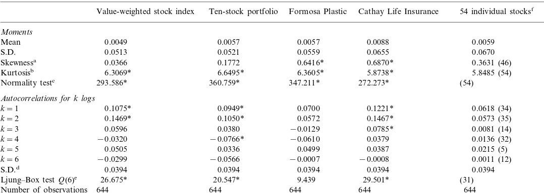
Table 1 shows summaries of statistical characteristics of weekly returns for all sample stocks and portfolios. To save spaces without losing generality, detailed results of individual stocks are shown only for the Formosa Plastic and the Cathay Life Insurance. For other individual stocks, only the number of stocks that pass a certain hypothesis test are shown in the table. For individual stocks, it is apparent that the weekly return distributions of almost all stocks have significant non-zero skewness and high-leveled kurtosis. Normality tests further confirm that stock returns in the Taiwan stock market are not normally distributed. In contract to the case of Brorsen and Yang (1994), Kim and Kon (1994), and De Santis and Imrohoroglu (1997), all the sample stock returns for the sample period in this study have their distributions positively skewed. This may be because our sample period contains the historical booming period from 1986 to 1989.

(12)

B

Summary statistics for stock returns for the period from January 1985 to May 1997

Cathay Life Insurance 54 individual stocksf

Value-weighted stock index Ten-stock portfolio Formosa Plastic Moments

Mean 0.0049 0.0057 0.0057 0.0088 0.0059

0.0670

Normality testc _293.586* _360.759* _347.211* _272.273* ₍₅₄₎

Autocorrelations for k logs

0.1221* 0.0618 (34)

k=1 0.1075* 0.0949* 0.0700

0.1469* 0.1050* 0.0572 0.0573 (35)

k=2 0.1467*

Ljung–Box testQ(6)e _26.675* _20.547* _9.439

644 644 644 644

644 Number of observations

* Denotes that the test is statistically significant at the level of 5%.

a_{Represents tests for hypotheses that the skewness is zero. Critical value is given in Pearson and Hartley (1975).} b_{Represents tests for hypotheses that the kurtosis is 3. Critical value is given in Pearson and Hartley (1975).}

c_{The statistic is}_{T·[(skewness}2_/₆₎₊_((kurtosis₋₃₎2_/_{24)] which is a}_x2_{distribution with 2 d.f. See Greene (1993). The critical value of the test is 5.99 at the}

significance level of 5%.

d_{The standard deviation (S.D.) of autocorrelations with log}_p_{is 1}_/_T. e_{The statistic is}_Q(6)₌_T(T₊₂₎

k=1 6 ₍_r

k

2₎_/_(T₋_{k) which is a}_x2_{distribution with 6 d.f. The critical value of the test is 12.59 at the significance level of}

5%.

f_{Numbers in this column are average values across the 54 individual sample stocks. Numbers in parentheses in this column are the number of stocks out}

(13)

distribution almost decays to a trivial level. This primary evidence implies that skewness might be diversified away, while the kurtosis is not diversifiable through the portfolio.

Finally, autocorrelations exist in many of the individual stock return series, and in all stock portfolios and the value-weighted stock index return series. This is consistent with the results of Kim and Kon (1994) which showed that the significant autocorrelation coefficients for the indexes are most likely a result of the nonsyn-chronous trading effect.

4. Empirical analysis

Tables 2 – 11 show the estimated coefficients for various models as well as tests of various hypotheses for each individual stock and portfolio return. To save space, we only show the detailed results for two individual stocks, the ten-stock portfolio, and the value-weighted stock index. We summarize the results for the 54 individual stocks in Tables 6 and 7.

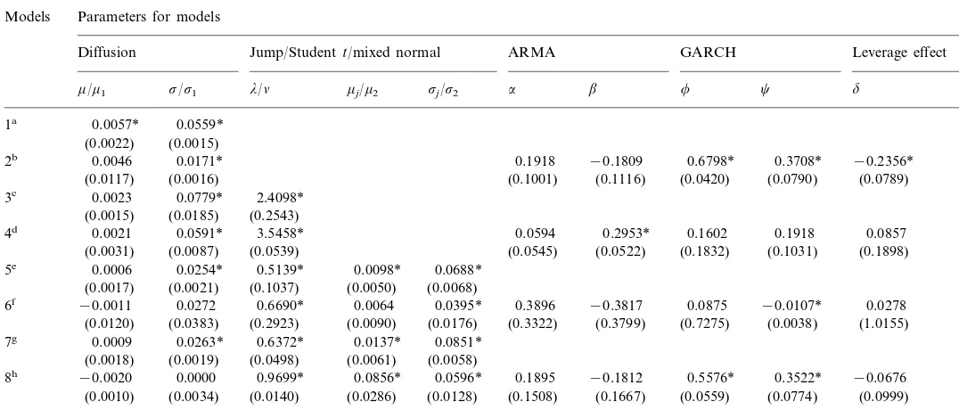
4.1. The case of indi6idual stocks

Table 2 and Table 3 are estimation results for the Formosa Plastic. In the stationary normal model (Section 2.1.1), the estimated parameters and the statisti-cal tests are consistent with those in Table 1. The skewness and kurtosis tests show the return distribution is not normal. The insignificant Ljung – Box Q(12) test for the standardized residual implies that autocorrelation does not exist in the stock return series. On the other hand, the Ljung – Box Q(12) test is significant for the squared standardized residual implying that autoregressive heteroscedasticity might exist in the stock return series. The result of Section 2.1.2 shows that the GARCH parameters are statistically significant. After including the GARCH process, the

volatility parameter s is significantly lower compared to that of Section 2.1.1,

meaning that a significant part of the volatility can be explained by the GARCH model. Moreover, there is a negative leverage effect on the return volatility in the case of Formosa Plastic. These GARCH factors account for a significant part of the return volatility, which can be judged from the low Ljung – Box Q(12) statistics for the squared standardized residual in Section 2.1.2. Both of the two ARMA parameters are not significant revealing that there is no autocorrelation existing in the return process, which is consistent with previous results. As a whole, the ARMA – GARCH model with the conditional normal distribution is significant

according to thex2_{test and the Schwarz criterion, while it is still unable to explain}

the skewness and excess kurtosis of the stock return distribution.

Since the conditional normal distribution seems unable to describe stock returns,

next we use the Student-t distribution. The result for Section 2.2.1 shows the d.f.

parameter for the model is 2.4 meaning the observed high kurtosis may be partly

captured by the parameter3_{. Although the model is superior to Sections 2.1.1 and}

3_{In order to explain the observed kurtosis relative to the stationary normal, the d.f. parameter for the}

(14)

B

Parameters estimation for various models (Formosa Plastic) Parameters for models

Models

GARCH Leverage effect

Diffusion Jump/Studentt/mixed normal ARMA

mj/m2 sj/s2 a b f c d

0.1918 −0.1809 0.6798* 0.3708* −0.2356* 2b _0.0046 _0.0171*

(0.0117) (0.0016) (0.1001) (0.1116) (0.0420) (0.0790) (0.0789)

0.0023 0.0779* 2.4098*

4d _0.0021 _0.0591* _3.5458* _0.0857

(0.0545) (0.0522) (0.1832) (0.1031) (0.1898) (0.0031) (0.0087) (0.0539)

0.0688* 0.0006 0.0254* 0.5139* 0.0098*

5e

(0.0017) (0.0021) (0.1037) (0.0050) (0.0068)

0.3896 −0.3817 0.0875 −0.0107* 0.0278 0.0395*

−0.0011

6f _0.0272 _0.6690* _0.0064

(0.0176)

(0.0120) (0.0383) (0.2923) (0.0090) (0.3322) (0.3799) (0.7275) (0.0038) (1.0155)

0.0009 0.0263* 0.6372* 0.0851*

−0.0020 0.0000 0.9699* 0.0856* 0.1895 −0.1812 0.5576* 0.3522* −0.0676 8h

(0.0010) (0.0034) (0.0140) (0.0286) (0.0128) (0.1508) (0.1667) (0.0559) (0.0774) (0.0999)

a_R

(15)

B

Statistical tests for various models (Formosa Plastic)

l(R,u) Standardized residual Squared standardized

Models x2_test _Schwarz

residual criterionh

Normality test Ljung–Box Ljung–Box Q(12)i

Excess kurtosis Skewness

Q(12)i

347.211* 11.5232 146.7104*

1 942.232 – 937.761 0.6416* 3.3605*

3.1303* 297.380* 5.8546 3.8633

1008.370 – 998.671 3.3605* 347.211* 11.5232 146.7104*

3 0.6416*

3.8505*

1011.013 x12=5.286 985.142 0.7788* 462.941* 0.4788 0.0004

4

3.3605* 347.211* 11.5232 146.7104* 0.6416*

5 1018.892 x22 1002.727

=153.32*,b

x52 0.6416* 3.3605* 347.211* 11.5232 146.7104*

1017.013

7 1000.848

=149.562*,e

x12=96.572*

1032.984 0.6809* 3.5703* 391.808* 5.8308 4.8721

x62

2_{is the statistic for the hypothesis test}_H

0:a=b=f=c=d=0 with the corresponding alternative Sections 2.1.2, 2.2.2 and 2.3.2 or Section 2.4.2 is

true. It is ax2_{distribution with 5 d.f.} b_x

2

2 _{is the statistic for the hypothesis test}_H

0:l=mJ=sJ=0 with the alternative that Section 2.3.1 is true. It is ax2 distribution with 3 d.f.

c_x 3

0:l=mJ=sJ=0 with the alternative that Section 2.3.2 is true. It is ax2 distribution with 3 d.f.

d_x 4

0:l=mJ=sJ=a=b=f=c=d=0 with the alternative that Section 2.3.2 is true. It is ax2distribution with 8 d.f.

e_x 5

0:l=m2=s2=0 with the alternative that Section 2.4.1 is true. It is ax2 distribution with 3 d.f. f_x

6

0:l=m2=s2=0 with the alternative that Section 2.4.2 is true. It is ax2 distribution with 3 d.f. g_x

7

0:l=m2=s2=a=b=f=c=d=0 with the alternative that Section 2.4.2 is true. It is ax2distribution with

8 d.f.

h_{The value of the Schwarz criterion is}_l

(R,u)−(1₂)p·ln (T), wherepis the number of parameters estimated in the model.

i_{The statistic is}_Q(12)₌_T(T₊₂₎

k=1 12 _[_r

k

2_/_(T₋_{k)] which is a}_x2_{distribution with 12 d.f. The critical value of the test is 12.59 at the significance level of}

5%.

(16)

2.1.2 based on the Schwarz criterion, it is unable to explain the conditional heterscedasticity in the return series. Section 2.2.2 is the combination of the

ARMA – GARCH and the Student-tmodel. The GARCH parameters in the model

are not significant. The chi-square test (x12) and the Schwarz criterion confirm that

Section 2.2.2 is not significant relative to Section 2.2.1. If the Student-t-GARCH

model generates the sample data, the standardized residuals should be an i.i.d.

Student-tdistribution. While, as shown in Table 3, the skewness for the

standard-ized residuals either for Section 2.2.1 or Section 2.2.2 is still significantly positive,

implying that the conditional distribution of stock returns may not be the Student-t

distribution. This is consistent with Brorsen and Yang (1994). Also, as noted by

Vlaar and Palm (1993), symmetric distributions such as the normal, Student-t or

generalized error distribution are unlikely to give appropriate results.

To deal with the skewness in stock return distribution, we examine several mixtures of normal distribution models. Section 2.3.1 is the Poisson – normal jump-diffusion model. According to Table 3, the model is superior to the previous

model. The chi-square test (x22) shows the model is better than the stationary

normal model. The Schwarz criterion shows it is better than any other previous

models. The mean parameter for jump magnitude (mJ) is positive consistent with

positive skewness of stock return distribution. With the jump component added to

the simple diffusion model (Section 2.3.1), the value ofsdecreases further, and the

value of m diminishes to a non-significant level. This means that the jump in the

stock price explains most of the mean and some portion of the volatility of stock returns. In Section 2.3.1, the mean and variance of stock returns can be found by

E(Rt)=m+lmJ and Var(Rt)=s 2₊_l₍_s

J 2₊_m

J

2_{), which would be equivalent to the}

mean and variance obtained in Section 2.1.1. The jump intensity parameter (l) in

Section 2.3.1 is estimated as 0.5139, which can be explained as, on average, a jump in stock returns happens every 2 weeks or so. The mean parameter for jump

magnitude (mJ) is estimated as 0.0098, which is significantly positive, consistent with

the positive skewness in the return distribution.

Unfortunately, Section 2.3.1 can not explain the conditional heteroscedasticity in the return process. Section 2.3.2 combines the ARMA – GARCH model and the Poisson – normal jump-diffusion model. Since both jump and GARCH components have been found in stock returns, the observed leptokurtosis in stock returns can be explained by either of the two models. The question arises as to which of the two processes provides a superior description of the data. The result shows the GARCH parameters are small and only one is significant compared to those from Section 2.1.2. Thus in Section 2.3.2, only a small part of conditional heterscedasitcity can be explained. This can be confirmed by the Ljung – Box test for the square standardized residual in Table 3. Overall Section 2.3.2 is still a’posteriori more probable than the previous models according the Schwarz criterion.

In the GARCH jump-diffusion model, Section 2.3.2, the GARCH parameters are small compared to those of Jorion (1988). The volatility parameter of the jump part is lower because it is partly explained by GARCH parameters. On the other hand,

the volatility parameter of the diffusion part is at the same level as in Section 2.3.14_.

4_{This is a general case for almost all of the sample individual stock and portfolio returns. This can}

(17)

This implies that in the GARCH jump-diffusion model, only the jump volatility is related to the conditional heteroscedasticity. This makes sense since volatility clustering happens when jumps happen in the return process. The results are very different from those of Jorion (1988) and others. Their models only allow the GARCH process in the diffusion part. Thus they accredit the conditional het-eroscedasticity to the diffusion part only. It is obviously not appropriate for the case of our study, since most of the conditional heteroscedasticity is associated with the jump part. Our model can consider the GARCH process for both the diffusion part and jump part and to tell which component is more related to GARCH. Our empirical results show the disadvantage of the Jorion (1988) model in that it is unable to explain the GARCH phenomenon in the jump process.

One of the probable reasons why the GARCH parameters are not significant in Section 2.3.2 is its complication in structure. In the Jorion (1988) model, the GARCH process is only in the diffusion part and the jump component is additional to the diffusion GARCH model. In Section 2.3.2, the GARCH is dependent upon the mixture of the jump component and the diffusion part. Presumably, the kurtosis of stock returns is largely explained by the Poisson jump diffusion model, thus leaving the GARCH factor non-significant. Moreover, since the probability density function of a Poisson jump diffusion distribution involves infinite summation, truncation errors as noted by Vlaar and Palm (1993) matter very much in Section 2.3.2. This complication may cause estimation errors resulting in non-significant GARCH parameters in Section 2.3.2.

Section 2.4.1 is the mixed – normal model that is similar to the Bernoulli jump model suggested by Ball and Torous (1983). This model has an advantage in its simplicity in structure. The probability density function can have an exact form rather than involving infinite summation as in the Poisson jump-diffusion model. The result shows the estimated parameters in Section 2.4.1 are all significant with the exception of one of the mean parameters. As Vlaar and Palm (1993) and Kim and Kon (1994) noted, the mixture of three normal distributions may be preferred. For parsimonious purposes, we only use the mixture of two normal distributions. This is especially desirable when we combine the mixture of normal distributions

and the GARCH model. In Section 2.4.1, m1 and m2 are significantly different

consistent with non-zero skewness in the return distribution. l is significantly

different from zero consistent with the high kurtosis in the return distribution. The

mean and variance of stock returns can be found by E(Rt)=lm1+(1−l)m2 and

Var(Rt)=ls12+(1−l)s22, which would be equivalent to the mean and variance

obtained in the Section 2.1.1. Section 2.4.2 shows that the combination of the

GARCH model and the mixed – normal model is the best model according to x2

tests and the Schwarz criterion. In Section 2.4.2, the two volatility parameters s1

and s2 are significantly lower than those of Section 2.4.1. This implies that a

(18)

whole normal – jump mixture, while their model, similar to Jorion (1988), only allows the GARCH phenomenon in the diffusion – normal component.

Why the GARCH parameters for the Student-tdistribution in Section 2.2.2 and

jump-diffusion process in Section 2.3.2 are insignificant is that they may absorb a large part of heteroscedasticity, explaining most of the kurtosis in the unconditional stock distribution.

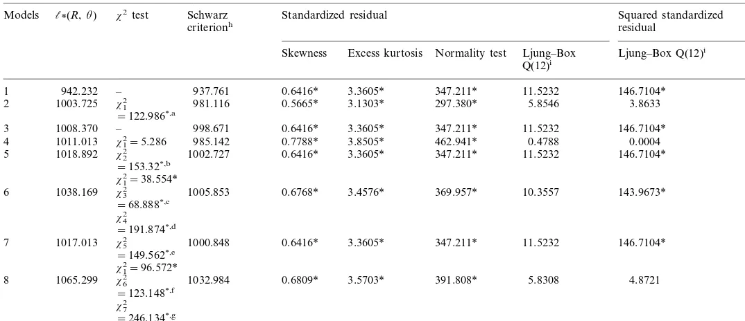
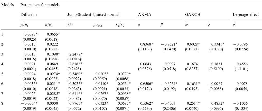
Table 4 and Table 5 show the results for another individual stock, Cathay Life Ins. The results are similar to those of the Formosa Plastic except that most ARMA parameters are significant, which is consistent with the results in Table 1 showing autocorrelation exists in the return series of the Cathay Life Ins. stock. Other detailed explanations are not repeated here.

As to other sample stocks, Table 6 and Table 7 summarizes the results for the 54 individual stocks. Most of the sample stocks show results similar to those of

Taiwan Plastic and Cathay Life Ins. Almost all sample stocks have their x2

tests significant at the level of 5% in any case. This implies that the normal distribution is not appropriate for individual stock returns. And the ARMA – GARCH model is significant under any of the four distributions assumed. Moreover, according to the Schwarz criterion, 39 out of the 54 sample stocks have their SC largest for Section 2.4.2, meaning that the mixed – normal – GARCH is the most probable model for individual stock returns. In addition, the leverage effect is not significant for most of the individual stocks.

4.2. The case of stock portfolios

Table 8 and Table 9 show the estimated coefficients and hypothesis tests for the

ten-stock portfolio returns5

. The results are different from those of individual stocks in some respects. First with respect to their jump behaviors in Section 2.3.1

and Section 2.3.2, the jump intensity parameter (l) is, in general, smaller than that

for most of the individual stocks, although it is still statistically significant. This might be because diversification can eliminate some jump risks in the portfolio. Moreover, with the jump component included in the model, the mean for the

diffusion model mdoes not change a lot, while the mean of jump size mJ becomes

non-significant from zero. Thus although the jump component persists, the jump becomes symmetric, and the mean of the jump magnitude is zero in a stock portfolio. In other words, the jump risk cannot be fully diversified, while the skewness is diversifiable through the portfolio.

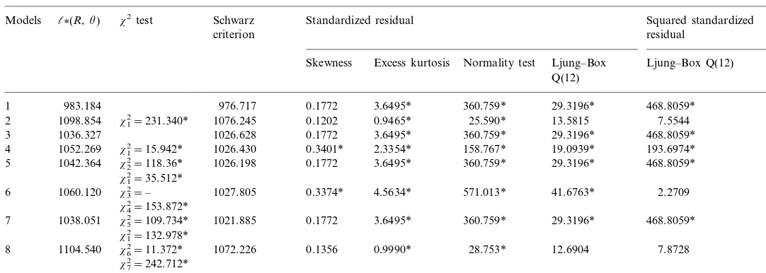
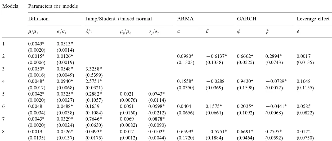
Table 10 and Table 11 show the results for the value-weighted stock index. The results are quite similar to those of the ten-stock portfolio. From the results of the stock portfolio, one can conclude that that in the Taiwan stock market, the jump and the GARCH components persist, while the jump size becomes symmetric in stock portfolios. In other words, although kurtosis cannot be fully diversified, skewness is diversifiable through the portfolio.

5_{This is one of our random portfolios from repeated experiments. To save space, other results for}

(19)

B

Parameters estimation for various models (Cathay Life Ins.) Models Parameters for models

ARMA Jump/Studentt/mixed normal

Diffusion

0.8368* −0.7521* 0.6028* 0.3343* −0.0796

2 0.0013 0.0222

(0.0010) (0.0222) (0.1163) (0.1470) (0.0621) (0.0720) (0.0724)

0.0018 0.1098* 2.2478* 3

(0.1816) (0.0298)

(0.0015)

4 0.0021 0.0649 2.6186* 0.0643 0.0097 0.1674 0.1831 0.4556

(0.0376) (0.0518) (0.8237) (0.5190) (1.3101) (0.0021) (0.0465) (0.2428)

0.0779*

−0.0024 0.0274* 0.5460* 0.0205* 5

(0.0018) (0.0023) (0.0922) (0.0059) (0.0068)

0.6506* −0.6254* 0.1631* −0.0067 0.0078 0.0534*

−0.0035*

6 0.0211* 0.3025* 0.0110*

(0.0033)

(0.0010) (0.0018) (0.0363) (0.0021) (0.0174) (0.0192) (0.0193) (0.0088) (0.0054) 0.0267* 0.0958*

7 −0.0025 0.0285* 0.6116*

(0.0057) (0.0485) (0.0070)

(0.0019) (0.0022)

0.0685*

−0.0054* 0.0000 0.7765* 0.0323* 0.5362* −0.4503 0.2514* 0.4852* −0.1056 8

(0.0107) (0.0071) (0.2230) (0.2406) (0.0640) (0.0995) (0.1334) (0.0019) (0.0045) (0.0572)

(20)

B

Statistical tests for various models (Cathay Life Ins.)a

Models _l_(R,_u₎ x2_test _Schwarz Standardized residual Squared standardized residual

criterion

Normality test Ljung–Box Ljung–Box Q(12) Excess kurtosis

Skewness

Q(12)

839.683 833.217 2.8738* 272.273* 40.1609* 208.5069*

1 0.6870*

3 906.346 896.647 0.6870* 2.8738*

167.550* 29.4607* 71.9340* 1.9789*

0.7629* 4 926493 x12=40.294* 900.653

2.8738*

928.371 x22=69.376* 912.206 0.6870* 272.273* 40.1609* 208.5069* 5

x12=50.702*

3.7705*

(21)

B

Parameters estimation for various models (54 individual stocks) Models Parameters for models

Diffusion Jump/Studentt/mixed normal ARMA GARCH Leverage

effect

0.3261 −0.2753 0.6862 0.2536 −0.0393

2 0.0034 0.0192

4 0.0026 0.0697 2.9238 0.0762 0.3095 0.1628 0.0777

(28) (31) (25) (21) (9)

(9) (53) (52)

0.0683

−0.0013 0.0280 0.8348 0.0089 5

(9) (53) (52) (38) (54)

0.4969 −0.4476 0.1087 −0.0163 0.0549 0.0505

7 −0.0004 0.0327 0.5707

(54)

(52) (38)

(49) (53)

0.0345

0.0171 0.0303 0.0760 0.0204 0.2492 −0.2072 0.5064 0.2978 −0.0140

8

(38) (54) (33) (31) (42) (38) (13)

(53)

(43) (48)

a_{See notes in Table 2.}

b_{Numbers in this table without brackets are the average values of the estimated coefficients for the 54 individual stocks.}

c_{Numbers in this table within brackets are the number of stocks that exhibit statistical significance for the estimated coefficients at a significance level of}

(22)

B

Statistical tests for various models (54 individual stocks)a

Standardized residual

x2_test _Schwarz _{Squared standardized}

l(R,u)

Models

criterion residual

Skewness Excess kurtosis Normality test Ljung–Box Ljung–Box Q(12) Q(12)

4 849.2544 x12: (43) 823.4148 0.5561 63.3415

(54) (11) (26) 921.3983 x12: (54) 889.0831 0.4735

8

(49) (54) (54) (4) (6)

x62: (54)x72: (54) [39]

[43]

a_{See notes in Table 3.}

b_{Numbers in this table without brackets are the average values of the estimated statistics for the 54 individual stocks.}

(23)

B

Parameters estimation for various models (ten-stock portfolio) Models Parameters for models

Diffusion

0.7020* −0.6627* 0.6515* 0.3162* −0.0017

2 0.0018 0.0123*

(0.0017) (0.0016) (0.2758) (0.2902) (0.0489) (0.0654) (0.0823)

0.0055* 0.0557* 3.2827* 3

(0.4766) (0.0048)

(0.0017)

4 0.0051* 0.0581* 2.8829* 0.0943* 0.0099 0.1495* 0.0996* 0.4984*

(0.0384) (0.4057) (0.0459) (0.0484) (0.0975) (0.0019) (0.0023) (0.0074)

0.0750* 0.0051* 0.0320* 0.3017* 0.0019

5

(0.0018) (0.0026) (0.0986) (0.0073) (0.0107)

0.5337* −0.5007* 0.1240* −0.0334* 0.0828* 0.0500*

0.0030*

6 0.0403* 0.0429* 0.0050

(0.0105)

(0.0013) (0.0017) (0.0209) (0.0066) (0.0164) (0.0149) (0.0243) (0.0008) (0.0158) 0.0075 0.0893*

0.0063 0.0481* 0.0726* 0.0019 0.6566* −0.6087* 0.6270* 0.3023* 0.0483 8

(0.0019) (0.0054) (0.2557) (0.2691) (0.0544) (0.0719) (0.0973) (0.0145) (0.0152) (0.0323)

(24)

B

Statistical tests for various models (ten-stock portfolio)a

l(R,u)

Models

criterion residual

Excess kurtosis Normality test Ljung–Box Ljung–Box Q(12) Skewness

1098.854 x12=231.340* 1076.245 0.9465* 25.590* 13.5815 7.5544

2 0.1202

360.759*

3 1036.327 1026.628 0.1772 3.6495* 29.3196* 468.8059*

158.767* 19.0939* 193.6974* 2.3354*

x12=15.942*

4 1052.269 1026.430 0.3401*

0.1772

x22=118.36* 3.6495* 360.759* 29.3196* 468.8059*

1042.364 1026.198

5

x12=35.512*

1027.805 0.3374* 4.5634* 571.013* 41.6763* 2.2709 1060.120 x32=–

6

x42=153.872*

(25)

.-Parameters estimation for various models (value-weighted stock index) Models Parameters for models

Diffusion

0.6980* −0.6137* 0.6662* 0.2894* 0.0017 2 0.0015* 0.0126*

(0.0006) (0.0019) (0.1303) (0.1338) (0.0525) (0.0743) (0.0135)

0.0050* 0.0548* 3.3258* 3

(0.5399) (0.0049)

(0.0016)

4 0.0048* 0.0940* 2.5751* 0.1558* −0.0288 0.9430* −0.0789* 0.1648

(0.0350) (0.0369) (0.1598) (0.0072) (0.1155) (0.0017) (0.0068) (0.0321)

0.0743* 0.0042* 0.0325* 0.2882* 0.0021

5

(0.0020) (0.0027) (0.1057) (0.0076) (0.0114)

0.0404 0.1575* 0.2035* −0.0441* 0.0585 0.0598*

0.0048

6 0.0488* 0.1639 0.0051

(0.0212)

(0.0034) (0.0038) (0.1084) (0.0160) (0.0656) (0.0661) (0.1092) (0.0068) (0.0822) 0.0069 0.0878*

0.0019 0.0526* 0.0493* 0.0017 0.6599* −0.5751* 0.6691* 0.2797* 0.0122 8

(0.0012) (0.0044) (0.1720) (0.1884) (0.0464) (0.0592) (0.0750) (0.0135) (0.0137) (0.0175)

(26)

B

Statistical tests for various models (value-weighted stock index)a

l(R,u)

Models

criterion residual

Excess kurtosis Normality test Ljung–Box Q(12) Ljung–Box Q(12) Skewness

293.586* 35.1577* 469.9958* 0.0366

1 992.830 986.364 3.3069*

1101.545 x1 1.3693* 50.419* 12.9823 8.9016

2₌_217.430* _1078.935

2 −0.0315

293.586*

3 1042.326 1032.627 0.0366 3.3069* 35.1577* 469.9958*

277.413* 56.9653* 492.918* 3.1975*

x12=119.502*

4 1102.077 1076.206 −0.1691

0.0366

x22=110.486* 3.3069* 293.586* 35.1577* 469.9958*

1048.073 1031.908

5

x12=35.634*

1033.550 −0.1056 3.6689* 362.396* 67.6949* 24.1971* 1065.890 x32=–

6

x42=146.42*

(27)

In the portfolio cases, skewness is not significant as shown in Table 1. The tendency of decreasing skewness as the size of the portfolio increases, implies skewness may be diversifiable. If the portfolio return is specified as the Poisson jump-diffusion

process, as shown in Table 8 and Table 9, the mean parameter mJ of the jump

magnitude becomes insignificant for both Section 2.3.1 and Section 2.3.2, meaning symmetric jumps exist in the portfolio return process. Similarly, if the portfolio return is specified as a mixed-normal process, as we can see in Table 8 and Table 10, the

mean parametersm1andm2for both Section 2.4.1 and Section 2.4.2 are not different

in magnitude. These results are consistent with the non-significant skewness in the portfolio return distribution. Moreover, according to Table 9 and Table 11, the

Schwarz criterion and chi-square testsx3

2

andx6

2

for Section 2.3.2 and Section 2.4.2 show that Section 2.1.2, the GARCH – normal model may be a reasonable model for portfolio return distribution.

5. Conclusion

In this study we investigated the distribution and conditional heteroscedasticity in stock returns on the Taiwan stock market. Apart from the normal distribution, in order to explain the leptokurtosis and skewness observed in the stock return

distribution, we also examined the Student-t, the Poisson – normal, and the mixed –

normal distributions, which are essentially a mixture of normal distributions, as the conditional distribution in the stock return process. We also used the ARMA (1,1) model to adjust the series autocorrelation, and adopted the GJR – GARCH (1,1) model to account for the conditional heterscedasticity exists in the return process. Extensive evidence was obtained by examining weekly returns for 72 individual stocks and the value-weighted stock index from January 1985 to May 1997. MLE was used to estimate parameters in various models, and the likelihood ratio test was used to test nested hypotheses.

The empirical results show that, first, stock returns can be best specified as the mixed – normal conditional distribution combined with the GARCH model. Second, the skewness may be diversified through the portfolio. Thus, the stock portfolio returns may be best specified by symmetric distributions, such as the normal or the

Student-t distribution combined with the GARCH model. Third, the continuous

mixture of normal, that is the Student-tdistribution, or the discrete mixture of an

(28)

References

Ahn, C.M., Thompson, H.E., 1988. Jump-diffusion processes and the term structure of interest rates. J. Finance 43 (1), 155 – 174.

Akgiray, V., Booth, G., 1986. Stock price processes with discontinuous time paths: an empirical examination. Financ. Rev. 21, 163 – 184.

Akgiray, V., Booth, G., 1988. Mixed diffusion-jump process modeling of exchange rate movements. Rev. Econ. Stat. 70, 631 – 637.

Amin, K.L., 1993. Jump diffusion option valuation in discrete time. J. Finance 48, 1833 – 1863. Ball, C.A., Torous, W.N., 1983. A simplified jump process for common stock returns. J. Financ.

Quantit. Anal. 18, 53 – 65.

Ball, C.A., Torous, W.N., 1985. On jumps in stock prices and their impact on call pricing. J. Finance 40, 155 – 173.

Blattberg, R.C., Gonedes, N.J., 1974. A comparison of the stable and student distribution as statistical models for stock prices. J. Bus. 47, 244 – 280.

Bollerslev, T., 1987. A conditionally heteroskedasticity time series model for speculative prices and rates of return. Rev. Econ. Stat. 69, 542 – 547.

Brorsen, B.W., Yang, S.-R., 1994. Nonlinear dynamics and the distribution of daily stock index returns. J. Financ. Res. 17 (2), 187 – 203.

Christie, A., 1982. The stochastic behavior of common stock variances: value, leverage, and interest rate effects. J. Financ. Econ. 10, 407 – 432.

Cox, J.C., Ross, S.A., 1976. The valuation of options for alternative stochastic processes. J. Financ. Econ. 3, 145 – 166.

Day, T.E., Lewis, C.M., 1992. Stock market volatility and the information content of stock index options. J. Econom. 52, 267 – 287.

De Santis, G., Imrohoroglu, S., 1997. Stock returns and volatility in emerging financial markets. J. Int. Money Finance 16 (4), 561 – 579.

Drost, F.C., Nijman, T.E., Werker, B.J.M., 1998. Estimation and testing in models containing both jumps and conditional heteroscedasticity. J. Bus. Stat. 16 (2), 237 – 243.

Duan, J.C., 1995. The GARCH option pricing model. Math. Finance 5, 13 – 32.

Duan, J.C., 1997. Augmented GARCH (p, q) process and its diffusion limit. J. Econom. 79, 97 – 127. Engle, R., 1982. Autoregressive conditional heteroskedasticity with estimates of the variance of united

kingdom inflation. Econometrica 50, 987 – 1007.

Engle, R., Ng, V., 1993. Measuring and testing the impact of news on volatility. J. Finance 48, 1749 – 1778.

Fama, E.F., 1965. The behavior of stock market prices. J. Bus. 38, 34 – 105.

Glosten, L.R., Jagannathan, R., Runkle, D., 1993. On the relation between the expected value and the volatility of the nominal excess return on stocks. J. Finance 48, 1779 – 1801.

Greene, W.H., 1993. Econometric Analysis, second ed. Prentice Hall, Inc.

Heston, S.L., 1993. A closed form solution for options with stochastic volatility with applications to bond and currency options. Rev. Financ. Stud. 6 (2), 327 – 343.

Hull, J.C., White, A., 1987. The pricing of options on assets with stochastic volatilities. J. Finance 42, 281 – 300.

Jarrow, R.A., Rosenfeld, E.R., 1984. Jump risks and the intertemporal capital asset pricing model. J. Bus. 57, 337 – 351.

Jorion, P., 1988. On jump processes in the foreign exchange and stock markets. Rev. Financ. Stud. 1 (4), 427 – 445.

Kim, D., Kon, S.J., 1994. Alternative models for the conditional heteroscedasiticy of stock returns. J. Bus. 67 (4), 563 – 598.

(29)

Merton, R.C., 1976. Option pricing when underlying stock returns are discontinuous. J. Financ. Econ. 3, 125 – 144.

Milhoj, A., 1985. The moment structure of ARCH models. Scand. J. Stat. 12, 281 – 292.

Nelson, D.B., 1991. Conditional heteroskedasticity in asset returns: a new approach. Econometrica 59, 347 – 370.

Nieuwland, F.G.M.C., Verschoor, W.F.C., Wolff, C.C.P., 1991. EMS exchange rates. J. Int. Financ. Markets Inst. Money 2, 21 – 42.

Pagan, A.R., Schwert, G.W., 1990. Alternative models for conditional stock volatility. J. Econom. 45, 267 – 290.

Pearson, E.S., Hartley, H.O., 1975. Biometrika Tables for Statisticians, vol. 1, third ed. Cambridge University Press, Cambridge.

Schwarz, G., 1978. Estimating the dimensions of a model. Ann. Stat. 6, 461 – 464.

Vlaar, P.J.G., Palm, F.C., 1993. The message in weekly exchange rates in the european monetary system: mean reversion, conditional heteroscedasticity, and jumps. J. Bus. Stat. 11 (3), 351 – 360.