Yang–Baxter Maps from the Discrete BKP Equation
⋆Saburo KAKEI †, Jonathan J.C. NIMMO ‡ and Ralph WILLOX §
† Department of Mathematics, College of Science, Rikkyo University,
3-34-1 Nishi-Ikebukuro, Toshima-ku, Tokyo 171-8501, Japan E-mail: [email protected]
URL: http://www.rkmath.rikkyo.ac.jp/∼kakei/index e.html
‡ Department of Mathematics, University of Glasgow, Glasgow G12 8QQ, UK
E-mail: [email protected]
URL: http://www.maths.gla.ac.uk/∼jjcn/
§ Graduate School of Mathematical Sciences, The University of Tokyo,
3-8-1 Komaba, Meguro-ku, Tokyo 153-8914, Japan E-mail: [email protected]
Received November 13, 2009, in final form March 19, 2010; Published online March 31, 2010
doi:10.3842/SIGMA.2010.028
Abstract. We construct rational and piecewise-linear Yang–Baxter maps for a general
N-reduction of the discrete BKP equation.
Key words: Yang–Baxter map; discrete BKP equation
2010 Mathematics Subject Classification: 37K10; 37K60; 39A10; 39A14
1
Introduction
Let Rbe a mapR :C2 →C2 and let Rij :Cn→Cn be the map that acts as R on thei-th and j-th factors in the direct product C× · · · ×Cand identically on the others. A map R is called a Yang–Baxter map if it satisfies the Yang–Baxter equation (with parameters) [23,24],
R12(λ1, λ2)R13(λ1, λ3)R23(λ2, λ3) =R23(λ2, λ3)R13(λ1, λ3)R12(λ1, λ2). (1)
An important example of a Yang–Baxter map can be derived from the 3D-consistency con-dition for the discrete potential KdV equation [17]:
R(κ, µ) : (u, v)7→
vp,u p
, p= 1 +κuv
1 +µuv, (2)
which is the HIIIB map in the classification of quadrirational Yang–Baxter maps found in [16] (which is in fact equivalent to the FIII map in the Adler–Bobenko–Suris classification [1]). An important property of the map (2) is that it is related to a geometric crystal of A(1)1 -type [5]. Indeed, if we set
u=eU/ǫ, v=eV /ǫ, p=eP/ǫ, κ=e−K/ǫ, µ=e−M/ǫ,
and take the ultra-discrete limit (henceforth “ud-limit”) ǫ → +0 [22], we obtain a piecewise-linear Yang–Baxter map,
(U, V)7→(V +P, U −P), P = max(0, U +V −K)−max(0, U +V −M), (3)
⋆This paper is a contribution to the Proceedings of the Workshop “Geometric Aspects of Discrete and
where we have used the formula
lim
ǫ→+0ǫlog e
A/ǫ+eB/ǫ
= max(A, B), A, B ∈R. (4)
It can be verified that (3) coincides with the combinatorial R-matrix of A(1)1 -type [6], and is in fact equivalent to the evolution rule of a soliton cellular automata (a box-ball system “with a carrier”) [20]. Furthermore, if we choose κ = 0, the map (2) coincides with Hirota’s discrete KdV equation [8] and is therefore related to the Takahashi–Satsuma soliton cellular automata [21] as discussed in [11].
In a previous paper [11], we showed how several Yang–Baxter maps can be directly obtained from the discrete KP hierarchy. The aim of the present paper is to investigate the BKP coun-terpart of this construction and of the map (2) in particular.
2
Hirota–Miwa equation and Harrison-type map
In this section, we briefly describe a non-autonomous version of the method that enabled us to obtain the map (2) from the Hirota–Miwa equation,
(b−c)τ(ℓ+ 1, m, n)τ(ℓ, m+ 1, n+ 1) + (c−a)τ(ℓ, m+ 1, n)τ(ℓ+ 1, m, n+ 1)
+ (a−b)τ(ℓ, m, n+ 1)τ(ℓ+ 1, m+ 1, n) = 0, (5)
which was introduced by Hirota [9]. The connection between (5) and the theA-type KP hierar-chy was clarified by Miwa [13]. A non-autonomous version of the Hirota–Miwa equation,
{b(m)−c(n)}τ(100)τ(011) +{c(n)−a(ℓ)}τ(010)τ(101)
+{a(ℓ)−b(m)}τ(001)τ(110) = 0, (6)
was studied in [25,26]. Here we have used the abbreviations, τ(100) =τ(ℓ+ 1, m, n),τ(101) = τ(ℓ+ 1, m, n+ 1), etc. The non-autonomous Hirota–Miwa (naHM) equation (6) arises as the compatibility condition for the linear system (cf. [3,14] for autonomous case),
ψ(010) = a(ℓ)
b(m)ψ(100) +
1− a(ℓ) b(m)
u(000)ψ(000),
ψ(001) = a(ℓ)
c(n)ψ(100) +
1− a(ℓ) c(n)
v(000)ψ(000), (7)
where u(ℓ, m, n),v(ℓ, m, n) are defined as
u(000) =τ(000)τ(110)
τ(100)τ(010), v(000) =
τ(000)τ(101)
τ(100)τ(001). (8)
We now impose the following 2-reduction condition with respect to the variableℓ;
u(ℓ+ 2, m, n) =u(ℓ, m, n), v(ℓ+ 2, m, n) =v(ℓ, m, n),
ψ(ℓ+ 2, m, n) =λψ(ℓ, m, n), a(ℓ+ 2) =a(ℓ) ∀ℓ∈Z. (9)
We furthermore require that the evolution in the remaining lattice directions is autonomous:
b(m) =b, c(n) =c ∀m, n∈Z. (10)
Then the linear system (7) is reduced to the 2×2 system
ψ0(m+ 1, n) ψ1(m+ 1, n)
=U(m, n)
ψ0(m, n) ψ1(m, n)
,
ψ0(m, n+ 1) ψ1(m, n+ 1)
=V(m, n)
ψ0(m, n) ψ1(m, n)
where ψi(m, n) =ψ(i, m, n) (i= 0,1) and the coefficient matrices U(m, n), V(m, n) are given by
U(m, n) =
{1−a(0)/b}u0(m, n) a(0)/b
λa(1)/b {1−a(1)/b}u1(m, n)
,
V(m, n) =
{1−a(0)/c}v0(m, n) a(0)/c
λa(1)/c {1−a(1)/c}v1(m, n)
,
uℓ(m, n) =u(ℓ, m, n), vℓ(m, n) =v(ℓ, m, n).
We remark that uℓ(m, n),vℓ(m, n) (ℓ= 0,1) obey the constraints
u0(m, n)u1(m, n) =v0(m, n)v1(m, n) = 1, (12)
under the conditions (9), (10). The discrete Lax equation
U(m, n+ 1)V(m, n) =V(m+ 1, n)U(m, n), (13)
follows from the compatibility condition for (11) and gives
uℓ(m, n)vℓ(m+ 1, n) =uℓ(m, n+ 1)vℓ(m, n), (14) {a(ℓ)−b}uℓ(m, n+ 1)− {a(ℓ)−c}vℓ(m+ 1, n)
={a(ℓ+ 1)−b}uℓ+1(m, n)− {a(ℓ+ 1)−c}vℓ+1(m, n), (15)
for ℓ = 0,1. Using (12) to eliminate the u1, v1 variables, one can solve (14) and (15) for u0(m, n+ 1) and v0(m+ 1, n), to obtain the 2-reduced non-autonomous discrete KP (na-dKP) equation,
u0(m, n+ 1) = ˜ F(m, n) v0(m, n)
, v0(m+ 1, n) = ˜ F(m, n) u0(m, n) ,
˜
F(m, n) = {a(1)−b}v0(m, n)− {a(1)−c}u0(m, n) {a(0)−b}u0(m, n)− {a(0)−c}v0(m, n)
. (16)
Alternatively, we can use (12), (14) and (15) to express u0(m, n + 1), v0(m, n) in terms of u0(m, n),v0(m+ 1, n):
u0(m, n+ 1) =v0(m+ 1, n)F(m, n), v0(m, n) =
u0(m, n) F(m, n),
F(m, n) = {a(1)−b}+{a(0)−c}u0(m, n)v0(m+ 1, n) {a(1)−c}+{a(0)−b}u0(m, n)v0(m+ 1, n)
. (17)
Motivated by (16) and (17), we define the following birational maps ˜R(b, c),R(b, c):
˜
R(b, c) : (u, v)7→ F˜ v,
˜ F u
!
, F˜= {a(1)−b}v− {a(1)−c}u
{a(0)−b}u− {a(0)−c}v, (18)
R(b, c) : (u, v)7→vF, u F
, F = {a(1)−b}+{a(0)−c}uv {a(1)−c}+{a(0)−b}uv.
i.e. it satisfies the Yang–Baxter equation with parameters (1). As discussed in [18], this is a direct consequence of the 3D-consistency of the discrete Lax equation (13). The solitonic map
˜
R(b, c) satisfies a similar but slightly different relation,
˜
R12(b, c) ˜R13(b, d)R23(c, d) =R23(c, d) ˜R13(b, d) ˜R12(b, c), (19)
which is also obtained from the 3D-consistency of the Lax pair.
Remark. Here we use the notation ˜R for “solitonic” maps and R for Yang–Baxter maps, whereas the opposite notation was used in [11].
If we impose theN-reduction conditions,
u(ℓ+N, m, n) =u(ℓ, m, n), v(ℓ+N, m, n) =v(ℓ, m, n),
ψ(ℓ+N, m, n) =λψ(ℓ, m, n), a(ℓ+N) =a(ℓ) ∀ℓ∈Z, (20) b(m) =b, c(n) =c ∀m, n∈Z,
instead of the 2-reduction conditions (9), (10), the resulting Yang–Baxter map are related to a geometric crystal of A(1)N−1-type [5]. Its ud-limit coincides with a combinatorial R-matrix of A(1)N−1-type and hence with the evolution rule for A(1)N−1-soliton cellular automata [6].
3
From the Miwa equation to Yang–Baxter maps
In [13], Miwa introduced a discrete analogue of the bilinear BKP equation,
(a+b)(a+c)(b−c)τ(100)τ(011) + (b+c)(b+a)(c−a)τ(010)τ(101)
+ (c+a)(c+b)(a−b)τ(001)τ(110) + (a−b)(b−c)(c−a)τ(111)τ(000) = 0. (21)
It is straightforward to generalize (21) to the non-autonomous case:
{a(ℓ) +b(m)} {a(ℓ) +c(n)} {b(m)−c(n)}τ(100)τ(011)
+{b(m) +c(n)} {b(m) +a(ℓ)} {c(n)−a(ℓ)}τ(010)τ(101) +{c(n) +a(ℓ)} {c(n) +b(m)} {a(ℓ)−b(m)}τ(001)τ(110)
+{a(ℓ)−b(m)} {b(m)−c(n)} {c(n)−a(ℓ)}τ(111)τ(000) = 0. (22)
The non-autonomous Miwa (naM) equation (22) arises as the compatibility condition for the linear system (cf. [4,15] for the autonomous case),
{a(ℓ) +b(m)}ψ(010)− {a(ℓ)−b(m)}u(000)ψ(110)
+{a(ℓ)−b(m)}u(000)ψ(000)− {b(m) +a(ℓ)}ψ(100) = 0, {a(ℓ) +c(n)}ψ(001)− {a(ℓ)−c(n)}v(000)ψ(101)
+{a(ℓ)−c(n)}u(000)ψ(000)− {c(n) +a(ℓ)}ψ(100) = 0,
where u(ℓ, m, n),v(ℓ, m, n) are defined as in (8).
We now impose theN-reduction condition (20) to obtain the discrete linear equations
U1(m, n)
ψ0(m+ 1, n) .. .
ψN−1(m+ 1, n)
=U2(m, n)
ψ0(m, n) .. . ψN−1(m, n)
, (23)
V1(m, n)
ψ0(m, n+ 1) .. .
ψN−1(m, n+ 1)
=V2(m, n)
ψ0(m, n) .. . ψN−1(m, n)
where ψi(m, n) =ψ(i, m, n) (i= 0,1) and the coefficient matricesUi(m, n), Vi(m, n) (i= 1,2) are given by
U1 =I+U(0)Λ, U2=U(0)+ Λ, U(0)= diag [β0u0, . . . , βN−1uN−1], V1 =I+V(0)Λ, V2 =V(0)+ Λ, V(0)= diag [γ0v0, . . . , γN−1vN−1], uℓ(m, n) =u(ℓ, m, n), vℓ(m, n) =v(ℓ, m, n),
Λ =
0 1
0 . .. . .. 1
λ 0
, βℓ=
b−a(ℓ)
b+a(ℓ), γℓ=
c−a(ℓ)
c+a(ℓ), (25)
where I is the identity matrix. We remark that uℓ(m, n), vℓ(m, n) (ℓ = 0,1, . . . , N−1) obey the constraints
u0(m, n)· · ·uN−1(m, n) =v0(m, n)· · ·vN−1(m, n) = 1, (26)
under the conditions (20). The compatibility condition of (23) and (24) is
U1(m, n+ 1)−1U2(m, n+ 1)V1(m, n)−1V2(m, n)
=V1(m+ 1, n)−1V2(m+ 1, n)U1(m, n)−1U2(m, n). (27)
We remark that detU1= detV1 = 1 + (−1)N−1λQN−1
j=0 βj and henceU1,V1 are invertible. To write down the Yang–Baxter map and the solitonic map associated with the discrete Lax equation (27), we use the abbreviations, uj := uj(0,0), vj := vj(0,0), ¯uj := uj(0,1), ¯
vj :=vj(1,0), u= (u0, . . . , uN−1),v = (v0, . . . , vN−1), ¯u= (¯u0, . . . ,u¯N−1), ¯v = (¯v0, . . . ,v¯N−1). Using these abbreviations, we have the following discrete evolution equations:
¯ uj =uj
fj+1(u,v) fj(u,v)
, v¯j =vj
fj+1(u,v) fj(u,v)
, j= 0,1, . . . , N−1,
fj(u,v) = N−1
X
k=0 k−1
Y
l=0
βj+lγj+luj+lvj+l(βj+kuj+k−γj+kvj+k). (28)
Here and in what follows, the subscripts are considered as elements of Z/NZ. One can show that the discrete Lax equation (27) is equivalent to
¯ uj =uj
gj(u,v)¯ gj+1(u,v)¯
, vj = ¯vj
gj+1(u,v)¯ gj(u,v)¯
, j= 0,1, . . . , N−1,
gj(u,v) =¯ N−1
X
k=0
(k−1 Y
l=0
γj+l¯vj+l·(βj+kγj+kuj+kv¯j+k−1)· N−1
Y
l=k+1
βj+luj+l
)
. (29)
We will give a derivation of the equations (28), (29) in Appendix A.
In analogy with (18) we shall refer to the equations (28) as a solitonic map: ˜
R(β,γ) : CN ×CN → CN ×CN
∈ ∈
(u,v) 7→ ( ¯u,v)¯
. (30)
The corresponding Yang–Baxter map is obtained from (29):
R(β,γ) : CN ×CN → CN ×CN
∈ ∈
(u,v)¯ 7→ ( ¯u,v)
R:
(U0, U1) ( ¯V0,V¯1)
+
(V0, V1) [image:6.612.116.460.358.457.2]( ¯U0,U¯1)
⇒
Figure 1. Graphical representation.
The birational map (31) satisfies the Yang–Baxter equation (1), whereas when considered to-gether, the Yang–Baxter map (31) and the BKP solitonic map (30) satisfy (19). We remark again that these “Yang–Baxter” properties are mere consequences of the 3D consistency of the discrete Lax equation (27).
Next we consider the ud-limit of the Yang–Baxter map (29), (31). To do this, we replace the parameters β andγ by
βj 7→√−1βj, γj 7→√−1γj, j= 0,1, . . . , N−1,
and introduce new independent variables Uj,Vj, ¯Uj, ¯Vj as defined in
eUj/ǫ =β
juj, eVj/ǫ =γjvj eU¯j/ǫ =βju¯j, eV¯j/ǫ =γjv¯j, j= 0,1, . . . , N−1. It follows from (26) thatPN−1
j=0 Uj =PNj=0−1U¯j andPj=0N−1Vj =PNj=0−1V¯j are independent ofm and n. Then taking the ud-limit of (29) gives
¯
Uj =Uj+Gj(U,V¯)−Gj+1(U,V¯),
Vj = ¯Vj+Gj+1(U,V¯)−Gj(U,V¯), j= 0,1, . . . , N−1,
Gj(U,V¯) = max 0≤k<N
k−1
X
l=0 ¯
Vj+1+ max(0, Uj+k+ ¯Vj+k) + N−1
X
l=k+1 Uj+l
!
, (32)
U = (U0, . . . , UN−1), V = (V0, . . . , VN−1), ¯
U = ( ¯U0, . . . ,U¯N−1), V¯ = ( ¯V0, . . . ,V¯N−1),
which defines a piecewise-linear Yang–Baxter mapR(ud):
R(ud) : RN → RN
∈ ∈
U,V¯ 7→ U¯,V .
We remark that if we impose the condition Uj,Vj¯ ≥ 0 (j = 0,1, . . . , N−1), the Yang–Baxter map R(ud) coincides with the combinatorial R-matrix of typeA(1)N−1 (see (2.12) in [19]).
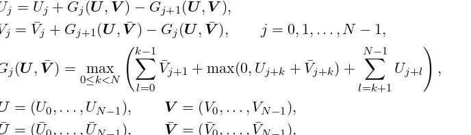
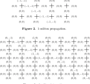
However, the piecewise-linear map (32) also admits soliton-type solutions in the general case. To describe these solitons, we use the notation of Fig. 1. Figs. 2 and 3 show soliton-type phenomena in the 3-reduced case, where we have set U0+U1+U2 = ¯U0 + ¯U1 + ¯U2 = 1 and
¯
V0+ ¯V1+ ¯V2=V0+V1+V2 = 0. The evolution shown in Fig.3is reminiscent of the interactions of solitons with stationary solutions that have been studied by Hirota in case of the ultra-discrete limit of the discrete Sawada–Kotera equation [10].
4
Concluding remarks
(−1,−1) (0,0) (0,0) (0,0)
(0,0)
+
(−1,−1)+
(0,0)+
(0,0)+
(0,0)(0,0) (−1,−1) (0,0) (0,0)
(0,0)
+
(0,0)+
(−1,−1)+
(0,0)+
(0,0)(0,0) (0,0) (−1,−1) (0,0)
Figure 2. 1-soliton propagation.
(0,−1) (0,0) (1,0) (0,0) (0,0) (0,0) (0,0) (0,0)
+
(0,−1)+
(0,0)+
(0,0)+
(0,0)+
(0,0)+
(0,0)+
(0,0) (0,−1) (1,0) (0,0) (0,0) (0,0) (0,0)(0,0)
+
(0,0)+
(0,−1)+
(0,0)+
(0,0)+
(0,0)+
(0,0)+
(0,0) (0,0) (1,−1) (0,0) (0,0) (0,0) (0,0) (0,0)+
(0,0)+
(0,0)+
(1,−1)+
(0,−1)+
(0,0)+
(0,0)+
(0,0) (0,0) (0,0) (1,0) (0,−1) (0,0) (0,0) (0,0)
+
(0,0)+
(0,0)+
(0,0)+
(0,0)+
(0,−1)+
(0,0)+
(0,0) (0,0) (0,0) (1,0) (0,0) (0,−1) (0,0) [image:7.612.165.466.59.342.2](0,0)
+
(0,0)+
(0,0)+
(0,0)+
(0,0)+
(0,0)+
(0,−1)+
(0,0) (0,0) (0,0) (1,0) (0,0) (0,0) (0,−1)Figure 3. 2-soliton interaction.
From the Lie-algebraic viewpoint, the (2n+1)-reduced BKP equation has the symmetry of the affine Lie algebra ofA(2)2n-type and the (2n)-reduced one has that ofD(2)n+1[2]. It is to be expected that the reduced ultra-discrete BKP system (32) is somehow related to crystal bases of the above types. However, in the 3-reduced case, our piecewise-linear map (32) seems to be different from the combinatorial R-matrix of A(2)2 -type, discussed explicitly in [7], as (32) has a rotational symmetry which theA(2)2 -type map in [7] does not possess. The exact relationship between the N-reduced discrete BKP equation andA(2)2 -type crystal bases needs further clarification.
A
Derivation of the
N
-reduced BKP equation
and related Yang–Baxter map
Here we give a derivation of the N-reduced BKP equation (28) and the related Yang–Baxter map (29).
In the caseN = 2, the nonlinear equations associated with the discrete Lax equation (27) are the same as in the 2-reducedA-case, i.e., those in Section2(as is to be expected for Lie-algebraic reasons). The first non-trivial example is the 3-reduced case and hereafter we assumeN ≥3.
Ifβj 6= 0, γj 6= 0 (j = 0,1, . . . , N −1) in (25), we can set βj =γj = 1 (j = 0,1, . . . , N−1) by rescaling the variables{uj},{vj}. In this appendix, we chooseβj =γj = 1.
We first remark that the inverse ofU1 of (25) is of the form,
U1−1 =
(
1 + (−1)N−1λ N−1
Y
i=0 βi
)−1
I+ N−1
X
j=1 (−1)j
j−1
Y
k=0 U(k)
!
Λj
where the matrices
have the properties,
U(k+N)=U(k), ΛU(k)=U(k+1)Λ, k= 0,1, . . . , N−1. (33)
We then introduce a degree on Mat(N), the space of N×N matrices:
∀X∈Mat(N) deg(X) =n ⇔ [d, X] =nX, d=N λ d
dλ−diag [1,2, . . . , N]. (34)
Substituting (33) into (27) and arranging in order of the degree (34), we obtain a set of equations foruj,vj, ¯uj, ¯vj. To write down these equations, we prepare some additional notation:
U = U(0),U(1), . . . ,U(N−1), V = V(0),V(1), . . . ,V(N−1),
¯
U = ¯U(0),U¯(1), . . . ,U¯(N−1)
, V¯ = ¯V(0),V¯(1), . . . ,V¯(N−1)
,
where ¯U(j) = U(j)(0,1), ¯V(j) = V(j)(1,0). We denote by hk U¯,VΛk the degree k terms in
(det ¯U1)(detV1) ¯U1−1U2V¯ 1−1V2, i.e.,
(det ¯U1)(detV1) ¯U1−1U2V¯ 1−1V2= 2N
X
k=0
hk U¯,V
Λk.
For example,h0 U¯,V,h1 U¯,V are given by
h0 U¯,V
= ¯U(0)V(0),
h1 U¯,V= ¯U(0) I − V(0)V(1)+ I −U¯(0)U¯(1)V(1).
By using this notation, the discrete Lax equation (27) can be rewritten as
hk U¯,V=hk V¯,U, k= 0,1, . . . ,2N. (35)
The system of polynomial equations (35) is of course overdetermined. However, it has a unique nontrivial solution. For the moment, we consider only two equations,
h0 U¯,V=h0 V¯,U, h1 U¯,V=h1 V¯,U. (36)
To solve (36), we introduce another set of variables [5,18]:
xj = j
Y
i=0
vk, x¯j = j
Y
i=0 ¯
vk, j= 0,1, . . . , N−2.
It is straightforward to show that~x=t[1 :x0:· · ·:xN−2]∈PN−1 satisfies a linear equation,
M~x=~0, (37)
M =
−u0v¯0p1 q0 −p0
−u1¯v1p2 q1 −p1
. .. . .. . ..
−uN−3¯vN−3pN−2 qN−3 −pN−3 −pN−2V −uN−2v¯N−2pN−1 qN−2
qN−1V −pN−1V −uN−1v¯N−1p0
Theorem 1. Assume that
ujv¯j 6= 1,
n
X
k=0
(k−1 Y
l=0 ¯
vj+l·(uj+kv¯j+k−1)· n Y l=k+1 uj+l ) 6
= 0, j= 0,1, . . . , N−1.(38)
Under this assumption, the space of solutions for the linear equation (37) is one-dimensional, and a basis is given by
t[1 :x
0 :x1 :· · ·:xN−2] =t[g0 : ¯v0g1: ¯v0v¯1g2 :· · ·: (¯v0· · ·v¯N−2)gN−1], (39)
where gj =gj(u,v) (j¯ = 0,1, . . . , N−1)are defined as (29).
To prove this theorem, we prepare two lemmas.
Lemma 1. Let Dn(m) be the determinant of order n:
Dn(m) =
qm −pm
−um+1¯vm+1pm+2 qm+1 . ..
. .. . .. −pm+n−2
−um+n−1¯vm+n−1pm+n qm+n−1
.
Then Dn(m) can be expressed as
Dn(m) = n−1
Y
i=1
(um+ivm+i¯ −1)· n X j=0
j−1
Y
k=0 ¯
vm+k·(um+jvm+j¯ −1)· n Y k=j+1 um+k . (40)
Proof . It is enough to prove the case m = 0. Using the recurrence relation Dn+2(0) = qn+1Dn+1(0)−un+1v¯n+1pnpn+2Dn(0), one can prove the Lemma1 by induction onn.
Lemma 2. detM = 0.
Proof . The desired result follows from (40) and a judicious expansion of M involving the
(N−1)-th andN-th rows.
Proof of Theorem 1. Denote by MN1 the matrix that results from M by deleting the N-th row and the first column. Under the assumption (38), detM1
N =DN−1(0)6= 0. Together with detM = 0 (Lemma 2), it follows that dim KerM = 1. The solution (39) can be checked by
direct substitution into (37).
Thus we have obtained (29). Next we will show that every relation in (35) holds if the variables u,v, ¯u, ¯v satisfy the relations (29).
Fora= (a0, . . . , aN−1),b= (b0, . . . , bN−1), we define polynomialsg(m)j (a,b) (j, m= 0,1, . . .,
N −1) as
gj(m)(a,b) = m
X
k=0
(k−1 Y
l=0
aj+l·(aj+kbj+k−1)· m Y l=k+1 bj+l ) .
Lemma 3. If the variables u,v, u,¯ v¯ obey the relation (29), then the following relations hold:
Proof . Since the equation is invariant under the rotation of the suffices, i.e. 0 7→ 1 7→ 2 7→ · · · 7→N−17→0, one can set j= 0 without loss of generality. The desired result can be proved by induction onm, using the recurrence relation
g0(m+1)(a,b) =g(m)0 (a,b)bm+ (a0· · ·am−1)(ambm−1).
A straightforward calculation shows that
h0 U¯,V=g0(0) U¯,V
+I,
h1 U¯,V
=−g(1)0 U¯,V,
hj U¯,V
= (−1)jng0(j) U¯,V+g(j−2)
0 U¯,V
o
, 2≤j≤N −1,
hN U¯,V
= (−1)N
(
¯
U(0)V(0)g1(N−2) U¯,V−g(N−2)
0 U¯,V
− N−1
Y
i=0 ¯ U(i)−
N−1
Y
i=0 V(i)
)
,
h2N−k U¯,V= (−1)k N−k
Y
i=0 ¯ U(i)V(i)
gN(k−−k+12) U¯,V (41)
+ (−1)k+1 N−k−2
Y
i=0 ¯ U(i)V(i)
gN(k)−k−1 U¯,V (2≤k≤N −1),
h2N−1 U¯,V= N−3
Y
i=0 ¯ U(i)V(i)
gN(1)−2 U¯,V,
h2N U¯,V
= N−2
Y
i=0 ¯ U(i)V(i)
.
Lemma 3 and relation (41) imply that the overdetermined system (35) is satisfied if the variables u, v, ¯u, ¯v obey the relation (29). In other words, this means that the discrete Lax equation (27) is equivalent to (29).
Just as the Yang–Baxter map (29) was shown to be equivalent to (36), under the condi-tion (38), the solitonic map (28) can also be shown to be equivalent to (36). We omit however the details of this proof.
Acknowledgments
The authors are grateful to Professors Atsuo Kuniba, Masato Okado, and Yasuhiko Yamada for discussions and comments. S.K. wishes to acknowledge support from the Japan Society for the Promotion of Science (JSPS) through a Grant-In-Aid for Scientific Research (No. 19540228); R.W. also acknowledges support by JSPS through a Grant-in-Aid (No. 21540210) and J.J.C.N. and R.W. acknowledge financial support from the British Council (PMI2 Research Co-operation award).
References
[1] Adler V.E., Bobenko A.I., Suris Yu B., Classification of integrable equations on quad-graphs. The consistency approach,Comm. Math. Phys.233(2003), 513–543,nlin.SI/0202024.
[2] Date E., Jimbo M., Kashiwara M., Miwa T., Transformation groups for soliton equations. Euclidean Lie algebras and reduction of the KP hierarchy,Publ. Res. Inst. Math. Sci.18(1982), 1077–1110.
[4] Date E., Jimbo M., Miwa T., Method for generating discrete soliton equations. V,J. Phys. Soc. Japan 52 (1983), 766–771.
[5] Etingof P., Geometric crystals and set-theoretical solutions to the quantum Yang–Baxter equation,Comm. Algebra31(2003), 1961–1973,math.QA/0112278.
[6] Hatayama G., Hikami K., Inoue R., Kuniba A., Takagi T., Tokihiro T., The A(1)M automata related to
crystals of symmetric tensors,J. Math. Phys.42(2001), 274–308,math.QA/9912209.
[7] Hatayama G., Kuniba A., Takagi T., Soliton cellular automata associated with crystal bases,Nuclear Phys. B
577(2000), 619–645,solv-int/9907020.
[8] Hirota R., Nonlinear partial difference equations. I. A difference analogue of the Korteweg–de Vries equation,
J. Phys. Soc. Japan43(1977), 1424–1433.
[9] Hirota R., Discrete analogue of a generalized Toda equation,J. Phys. Soc. Japan 50(1981), 3785–3791. [10] Hirota R., Ultradiscretization of the Sawada–Kotera equation, in Mathematics and Physics in Nonlinear
Waves (November 6–8, 2008, Fukuoka, Japan), Reports of RIAM Symposium, Vol. 20ME-S7, Research Institute for Applied Mechanics, Kyushu University, 2009, 76–85 (in Japanese).
[11] Kakei S., Nimmo J.J.C., Willox R., Yang–Baxter maps and the discrete KP hierarchy,Glasg. Math. J.51 (2009), no. A, 107–119.
[12] Maillet J.M., Nijhoff F.W., Integrability for multidimensional lattice models, Phys. Lett. B 224 (1989), 389–396.
[13] Miwa T., On Hirota’s difference equations,Proc. Japan Acad. Ser. A Math. Sci.58(1982), 9–12.
[14] Nimmo J.J.C., Darboux transformations and the discrete KP equation,J. Phys. A: Math. Gen.30(1997), 8693–8704.
[15] Nimmo J.J.C., Darboux transformations for discrete systems,Chaos Solitons Fractals11(2000), 115–120. [16] Papageorgiou V.G., Suris Yu.B., Tongas A.G., Veselov A.P., On quadrirational Yang–Baxter maps,
arXiv:0911.2895.
[17] Papageorgiou V.G., Tongas A.G., Veselov A.P., Yang–Baxter maps and symmetries of integrable equations on quad-graphs,J. Math. Phys.47(2006), 083502, 16 pages,math.QA/0605206.
[18] Suris Yu.B., Veselov A.P., Lax matrices for Yang–Baxter maps,J. Nonlinear Math. Phys.10(2003), suppl. 2, 223–230,math.QA/0304122.
[19] Takagi T., Soliton cellular automata, in Combinatorial Aspect of Integrable Systems,MSJ Mem., Vol. 17, Math. Soc. Japan, Tokyo, 2007, 105–144.
[20] Takahashi D., Matsukidaira J., Box and ball system with a carrier and ultradiscrete modified KdV equation,
J. Phys. A: Math. Gen.30(1997), L733–L739.
[21] Takahashi D., Satsuma J., A soliton cellular automaton,J. Phys. Soc. Japan 59(1990), 3514–3519. [22] Tokihiro T., Takahashi D., Matsukidaira J., Satsuma J., From soliton equations to integrable cellular
au-tomata through a limiting procedure,Phys. Rev. Lett.76(1996), 3247–3250.
[23] Veselov A.P., Yang–Baxter maps and integrable dynamics, Phys. Lett. A 314 (2003), 214–221, math.QA/0205335.
[24] Veselov A.P., Yang–Baxter maps: dynamical point of view, in Combinatorial Aspect of Integrable Systems,
MSJ Mem., Vol. 17, Math. Soc. Japan, Tokyo, 2007, 145–167,math.QA/0612814.
[25] Willox R., Tokihiro T., Satsuma J., Darboux and binary Darboux transformations for the nonautonomous discrete KP equation,J. Math. Phys.38(1997), 6455–6469.
[26] Willox R., Tokihiro T., Satsuma J., Nonautonomous discrete integrable systems, Chaos Solitons Fractals