getdoccdb2. 305KB Jun 04 2011 12:04:59 AM

(1)

El e c t ro n ic

Jo ur n

a l o

f P

r o b

a b i l i t y Vol. 11 (2006), Paper no. 10, pages 276–300.

Journal URL

http://www.math.washington.edu/~ejpecp/

Computation of Greeks using Malliavin’s calculus in

jump type market models

Marie-Pierre BAVOUZET-MOREL INRIA Rocquencourt

Domaine de Voluceau-Rocquencourt Projet MATHFI, 78150 Le Chesnay

[email protected]

Marouen MESSAOUD IXIS, 47 quai d’Austerlitz

75648 Paris Cedex 13

and INRIA Rocquencourt, Projet MATHFI [email protected]

Abstract

We use the Malliavin calculus for Poisson processes in order to compute sensitivities for European and Asian options with underlying following a jump type diffusion.

The main point is to settle an integration by parts formula (similar to the one in the Malliavin calculus) for a general multidimensional random variable which has an absolutely continuous law with differentiable density. We give an explicit expression of the differential operators involved in this formula and this permits to simulate them and consequently to run a Monte Carlo algorithm.

Key words: Malliavin calculus, Monte-Carlo algorithm, Euler scheme, compound Poisson process, sensitivity analysis, European options, Asian options.

AMS 2000 Subject Classification: Primary 60H07, 60J75, 65C05.

(2)

1 Introduction

In the last years, following the pioneering papers [9],[8] a lot of work concerning the numerical applications of the stochastic variational calculus (Malliavin calculus) has been done. This mainly concerns applications in mathematical finance: computations of conditional expectations (which appear in the american option pricing, for example) and of sensitivities (the so called Greeks). The models at hand are usually log-normal type diffusions and then one may use the standard Malliavin calculus. But nowadays people are more and more interested in jump type diffusions (see [5]) and then one has to use the stochastic variational calculus corresponding to Poisson point processes. Such a calculus has already been developped in [2] concerning the noise coming from the amplitudes of the jumps and in [4] concerning the jump times. More recently [3] gives a unified approach using the language of the Dirichlet forms. Another point of view, based on chaos decomposition may be found in [7], [1], [12], [14] and [11].

The aim of our paper is to give a concrete application of the Malliavin calculus approach for sensitivity computations (Greeks) for jump diffusion models. We give two examples: in the first one, we use the Malliavin calculus with respect to the jump amplitudes. In the second one, we add a Brownian part and differentiate with respect to both the jump amplitudes and to the Wiener increments.

The Malliavin integration by parts formula used in this paper is an elementary one. Notice that any numerical scheme used in a Monte Carlo algorithm appears as a function of a finite number of random variablesH₁, . . . , Hn. It turns out that, if the law of these random variables

is absolutely continuous with respect to the Lebesgue measure and has a smooth density, then the strategy developed in the Malliavin calculus may be implemented for H1, . . . , Hn and an

integration by parts formula is derived. This is not specific for the Brownian motion or for a Poisson point process but represents an elementary abstract calculus.

(3)

2 The problem

We compute the sensitivities of an option with payoff φ, where the asset (St)t≥0 follows a

one-dimensional jump diffusion process driven by a compound Poisson process. Let us precise our problem.

LetN be a compound Poisson process. We denote by (Ti)i∈Nthe jump times oft→N_t, and by

(Jt)t≥0 the corresponding standard Poisson process with parameterλ >0, that is Jtcounts the

number of jumps up to t and for all n≥1, Tn−Tn−1 has exponential distribution with mean

λ. For all i∈N∗_{, we define ∆}_i₌NTi−NTi−1, so ∆i represents the jump amplitude at timeTi. The random variables (∆i)i∈N∗ are independent and identically distributed. We assume that

the law of ∆i is absolutely continuous with respect to the Lebesgue measure and we denote by

ρ its density, that is ∆i∼ρ(a)da, for all i∈N∗.

We deal with two models. In the first one, the assetSt is a pure jump diffusion solution of the

SDE

In the second one, we add a Brownian part :

St=β+ a Malliavin calculus approach is used. We will follow a similar strategy in our frame, using Malliavin calculus for jump type diffusions. In the case of European option for example, we write

solve a deterministic integral equation. In the examples that we consider in this paper, the solutions of these equations are explicit, so that this term is explicitly known. Concerning the Merton’s model (2), we use the integration by parts formula of the standard Malliavin calculus (based on the Wiener increments) and we obtain

(4)

Assume now that JT =n 6= 0. Then, using an integration by parts formula on {JT = n}, we

where Hn is a weight involving “Malliavin derivatives” of ST and of ∂S_∂βT. These differential

operators are similar to those in [2], but the frame here is much more simple, since there are no accumulation of small jumps. So we will derive this integration by parts formula using elementary arguments. We obtain

∞

In order to employ this formula in a Monte-Carlo algorithm, we proceed as follows: we simulate the jump times (T_ni)n∈N,i= 1, . . . , M and the jump amplitudes (∆i_n)n∈N,i= 1, . . . , M, and we

In the case of Merton’s model we proceed as follows: we first simulate the jump timesTi, i∈N.

Once they are fixed we construct an Euler scheme in which the times Ti, i ∈ N are included

in the discretization grid. Then we simulate the amplitudes of the jumps and the Brownian increments and we thus perform the Monte-Carlo algorithm.

3 Malliavin calculus for simple functionals

On a probability space (Ω,F, P) we consider a sequence of independent random variables (Vn, n∈N∗). We suppose that for alln≥1,Vn has moments of any order.

Hypothesis 3.1 For every n ∈ N∗_{, the law of} Vn is absolutely continuous with respect to the

Lebesgue measure and has the densitypn which is continuously differentiable onRand such that

for all k ∈ N_, _lim

We introduce some notations. For k ≥ 1, we denote by Ck

↑(Rn) the space of the functions f : Rn_→R_{which are k times differentiable and such that f and its derivatives up to order k have}

at most polynomial growth. For a multi-index α= (α1, . . . , αk) we denote∂αkf =

∂k ∂α1. . . ∂αk

(5)

In the case k = 0, C0

↑(Rn) denotes the set of the functions f : Rn → R which are continuous with respect to each argument and have at most polynomial growth.

We define now the simple functionals and the simple processes.

A random variable F is called a simple functional if there exists some n ∈ N∗ _{and some}

measurable functionf : Rn_→R such that

F =f(V1, . . . , Vn).

We denote byS₍n,k) the space of the simple functionals such thatf ∈ C↑k(Rn). A simple process of lengthnis a sequence of random variables

U = (Ui)i≤n such that

Ui =ui(V1(ω), . . . , Vn(ω)).

We denote by P₍_n,k₎ the space of the simple processes of length n such that ui ∈ C_↑k(Rn), i=

1, . . . , n. Note that if U ∈P₍n,k) thenUi ∈S(n,k),i∈N∗.

We define now the differential operators which appear in the Malliavin’s calculus. The Malliavin derivative D:S₍_n,₁₎→P₍_n,₀₎:

ifF =f(V1, . . . , Vn), then

DiF := ∂if(V1(ω), . . . , Vn(ω)) =

∂f ∂xi

(V1(ω), . . . , Vn(ω)),

DF := (DiF)i≤n∈P(n,0).

The Skorohod integralδ :P₍n,1)→S(n,0):

δ(U) := −

n

X

i=1

(DiUi+θi(Vi)Ui)

= −

n

X

i=1

∂ui

∂xi

(V1, . . . , Vn) +θi(Vi)ui(V1, . . . , Vn)

,

with

θi(y) := ∂yln(pi)(y) = (p

′

i

pi)(y) ifpi(y)>0,

:= 0 ifpi(y) = 0.

Remark 3.1 For everyp∈N _{and for every} F ∈S₍_n,₁₎ and U ∈P₍_n,₁₎, one has

E

 

n

X

j=1

|DjF|2

 

p

<∞ and E (|δ(U)|p)<∞.

This comes from the following hypothesis: E|Vi|p <∞, for all i and f, ui, and ∂ln(pi), i =

1, . . . , n, have at most polynomial growth.

(6)

Proposition 3.1 Let F ∈S₍_n,₁₎ and U ∈P₍_n,₁₎ then

the last equality being obtained by integration by parts, where we have used that for allk∈N_,

lim

Suppose that F, G∈S₍_n,₂₎ then, as an immediate consequence of the duality relation (3) one obtains

E(F LG) =E(< DF, DG >) =E(G LF). (5) Moreover, the standard differential calculus rules give the following chain rule.

(7)

Finally, givenF = (F1, . . . , Fd), Fi∈S₍_n,₁₎, we introduce the Malliavin covariance matrix

We are now able to state the integration by parts formula.

Theorem 3.1 Let F = (F1, . . . , Fd₎ _∈ _Sd

(n,2), G ∈ S(n,1). We assume that the matrix σF is

invertible and denoteγF :=σF−1.

We also suppose that

E (detγF)4

Then the duality relation gives

(8)

By hypothesis (8), the above expectations are finite, so the proof is complete.

4 Integration by parts with respect to the jump amplitudes

In this section we use the integration by parts formula (9) with respect to ∆i∼ρ(a)da,i∈N∗,

which are the amplitudes of the jumps of (Nt)t≥0. Let (St)t≥0 be solution of the SDE

St=β+ Jt

X

i=1

c(Ti,∆i, STi−) +

Z t

0

b(r, Sr)dr . (11)

We work under the following hypothesis.

Hypothesis 4.1 ρ is continuously differentiable, ρ

′

ρ has at most polynomial growth on R and

for allk∈N_, _lim

y→±∞|y|

k

ρ(y) = 0.

Hypothesis 4.2 The functions (a, x) → c(t, a, x) and x → b(t, x) are twice continuously

differentiable and there exists a constant K >0 and α∈N _{such that:}

i)|c(t, a, x)| ≤K(1 +|a|)α(1 +|x|)

|b(t, x)| ≤K(1 +|x|)

ii)|∂xc(t, a, x)|+

∂_x2c(t, a, x)

+|∂_ac(t, a, x)| ≤K(1 +|a|)α

|∂xb(t, x)|+

∂_x2b(t, x) ≤K

Hypothesis 4.3 There existsη >0 such that

|∂ac(t, a, x)| ≥η >0.

4.1 The deterministic equation

We introduce the following deterministic equation.

We fix some 0 < u₁ < . . . < un < T, and we denote u = (u1, . . . , un). We also fix a =

(a1, . . . , an)∈Rn. To u and awe associate the equation

st=β+ Jt(u)

X

i=1

c(ui, ai, s_u−

i ) +

Z t

0

b(r, sr)dr,0≤t≤T , (12)

whereJt(u) =k ifuk ≤t < uk+1.

We use this deterministic equation in order to express St as a simple functional: on {Jt =n}

one has

St = st(T1, . . . , Tn,∆1, . . . ,∆n),

∂∆iSt = ∂aist(T1, . . . , Tn,∆1, . . . ,∆n), ∂_∆2_j_,_∆_iSt = ∂a2j,aist(T1, . . . , Tn,∆1, . . . ,∆n),

(9)

(10)

Proof. (i) Proceed by recurrence using hypothesis4.2 in (12), (13), (14), (15), and in (16).

4.2 Integration by parts formula

We come back to the problem developed in section 1 and we deal with equation (9). In the case of European options, we write

E

invertible and that (8) holds true, and then we compute

Hn(F, G) =G γFLF −γFhDF, DGi −GhDF, DγFi. (17)

So we can use Theorem 3.1 and we obtain the integration by parts formula (9). For the computation of the terms involved in the right hand side of (17),

• we use (13) forDF and γF, (16) forG, (13) and (14) forLF, (13), (14) and (15) forDγF,

• we differentiate with respect toaj in (16) to obtain DG.

In the case of Asian options, the numerical example treated in this paper (see section6.3) allows us to write for each fixedn∈N∗_{, on}_{JT =n},

exactly as before and obtain (17) with

(11)

5 Merton Process and Euler scheme

In this section we deal with the Merton model:

St=β+ Jt

X

i=1

c(Ti,∆i, S_T−

i ) +

Z t

0

b(u, Su)du+

Z t

0

σ(u, Su)dWu,

whereρ, b and c satisfy the previous hypothesis4.1,4.2 and4.3. Moreover, we assume

Hypothesis 5.1 The function x→σ(u, x) is twice continuously differentiable and there exists

two constantsC >0 and ǫ >0 such that:

i)|σ(u, x)| ≤C(1 +|x|), ii)|∂xσ(u, x)|+

∂_x2σ(u, x) ≤C ,

iii)|σ(u, x)| ≥ǫ .

We will present two alternative calculus for this model. The first one is based on the Brownian motion only and the second one is based on both the Brownian motion and the jump amplitudes. Suppose that the jump timesT1< . . . < Tnare given (this means that we have already simulated

T₁, . . . , Tn in the Monte-Carlo algorithm). We include them in the discretization grid: so we

consider a time grid 0 = t0 < t1 < . . . < tm < . . . < tM = T and we assume that Ti = tmi, i= 1, . . . , n for some m1 < . . . < mn. Fort >0, we denote m(t) = m if tm ≤t < tm+1. Then

the corresponding Euler scheme is given by

ˆ

St=β+ Jt

X

i=1

c(Ti,∆i,SˆT_i₋) + m(t)−1

X

k=0

σ(tk,Sˆtk) (Wtk+1−Wtk)

+

m(t)−1

X

k=0

b(tk,Sˆtk)(tk+1−tk).

This corresponds to the deterministic equation :

ˆ

st=β+ Jt

X

i=1

c(ui, ai,sˆ_u−

i ) +

m(t)−1

X

k=0

σ(tk,ˆstk) ∆kw+

m(t)−1

X

k=0

b(tk,sˆtk) (tk+1−tk), (18)

where we have denoted by ∆kw=wtk+1−wtk. So on {Jt=k}, one has ˆ

St= ˆst(T1, . . . , Tk,∆1, . . . ,∆k,∆0W, . . . ,∆m(t)−1W),

where ∆kW =Wtk+1−Wtk. Moreover we have :

∂∆iSˆt = ∂aisˆt(T1, . . . , Tk,∆1, . . . ,∆k,∆0W, . . . ,∆m(t)−1W), ∂_∆2_j_,_∆_iSˆt = ∂a2j,aisˆt(T1, . . . , Tk,∆1, . . . ,∆k,∆0W, . . . ,∆m(t)−1W),

∂βSˆt = ∂βsˆt(T1, . . . , Tk,∆1, . . . ,∆k,∆0W, . . . ,∆m(t)−1W),

(12)

The first derivatives of ˆst satisfy the following equations :

For the derivatives of higher order one may derive similar equations. Now we have the choice of using the integration by parts formula from the section 2, using ∆iW or both ∆i and ∆iW.

And in each case we have different forms for the differential operators. For example on the set

{Jt=k}

so that the corresponding LW

i is given by

Then the Ornstein-Uhlenbeck operator will be

(13)

Notice that if m=m(t)

σ_tJ,W ≥σW_t ≥ ∂_∆_m

−1Wsˆt

2

=

σ(t_m₋₁,sˆ_t_m

−1)

2

≥ǫ2 >0.

This allows us to use the integration by parts formula corresponding to the Brownian motion only, or to both Brownian motion and jump amplitudes (the first case leads to the same calculus as in [6] and [13]). It is more delicate to prove the non degeneracy condition (8) if we only use the jumps.

6 Numerical results

We compute here the Delta of two European and Asian options (call option with payoffφ(x) = (x−K)+and digital option with payoffφ(x) =1x≥K) with underlying (St)t≥0 following a jump

type diffusion model.

LetN be a compound Poisson process with jump intensityλ. For all i∈N∗, we denote ∆i the

jump amplitude ofN at the jump time Ti. We suppose that ∆i ∼ N(0,1),i≥1.

We deal with two different jump diffusion models. The first one is motivated by Vasicek’s model for interest rates (but we consider a jump process instead of a Brownian motion):

St=S0−

Z t

0

r(Su−α)du+σ Jt

X

i=1

∆i. (25)

The second one is of Black-Scholes type:

St=S0+

Z t

0

r Sudu+σ Jt

X

i=1

S_T−

i ∆i, (26) We compare the different Monte Carlo estimators of the Delta, obtained by using

• Finite difference method

• Malliavin calculus

• localized Malliavin calculus.

Remark 6.1 Values of the parameters.

The numerical results are given in figures 3, 5, 4, 6, 7 and 8. We denote by σV and σBS the

parameters corresponding to the Vasicek model (25) and the geometric model (26) respectively.We choose ‘large’ values forσV (σV = 20in the numerical results) in order to fit the values usually

used by the practiciens in the Vasicek model. On the contrary, we take weak values for σBS

(σBS = 0.2 in the numerical results) in order to fit the usual values of the volatility in the

(14)

6.1 Localization method

For European and Asian call options, we use the same variance reduction method as the one introduced in [9]. For European options, sensitivity analysis using Malliavin calculus leads to terms such as φ(ST), Hn(ST,

∂ST

∂β ) (take IT for ST in the case of Asian options), which may

have a large variance. It is possible to avoid this problem by using a localizing function which vanishes out of an interval [K−δ , K+δ], for someδ >0. Let us introduce some notations.

Bδ(s) := 0 ifs≤K−δ

:= s−(₂K_δ−δ) ifs∈[K−δ , K+δ]

:= 1 ifs≥K+δ ,

and

Gδ(t) :=

Rt

−∞Bδ(s)ds

:= 0 ift≤K−δ

:= (t−(K₄_δ−δ))2 ift∈[K−δ , K+δ] := t−K ift≥K+δ .

Note thatBδ is the derivative of Gδ. We define

Fδ(t) := (t−K)+−Gδ(t)

:= 0 ift≤K−δ

:= −(t−(K₄_δ−δ))2 ift∈[K−δ , K] := t−K− (t−(K₄−_δδ))2 ift∈[K, K+δ]

:= 0 ift≥K+δ

Since Fδ(ST) +Gδ(ST) = (ST −K)+, we have on {JT =n},

∂βE [(ST −K)+] =

∂

∂βE [Gδ(ST)] + ∂

∂βE [Fδ(ST)]

= E [Bδ(ST)∂βST] + E [Fδ(ST)Hn(ST, ∂βST)] .

SinceFδ vanishes out of [K−δ, K+δ], the value of the second expectation does not blow up as

Hn increases.

6.2 Finite Difference method

Arbitrage theory gives an expression for the price u(,) of an option, with underlying S and payoffφ, as the following expected value :

u(0, S0) = E [φ(ST)|S0].

To compute the Delta, the finite difference method makes a differentiation using the Taylor expansion of the price with respect toS0. Indeed, we shiftS0 withǫand compute the new price

u(0, S0+ǫ), then the first term of the Taylor expansion of the price around S0 is given by:

∂u(0, S₀)

∂S0 ≃

u(0, S₀+ǫ)−u(0, S₀−ǫ)

2ǫ .

(15)

6.3 Malliavin estimator

We recall that we have computed the Delta estimator using Malliavin integration by parts formula (see section 2):

E

• We first study the diffusion process defined by (25). We have an explicit expression of ST on

{JT =n}:

In order to compute the Malliavin derivatives ofST involved in the weightHJT, we differentiate with respect to the jump amplitudes in (27). Thus, for all 1≤i≤n, one has

and the covariance matrix is defined by :

(16)

• We study the jump diffusion process defined by (26). matter of notation. Let us define

Aσ =

Hence, for European options

(17)

with the conventionT0= 0 and Tn+1 =T. For all t∈[Tj, Tj+1[,

Hence, for Asian options

H_nA(IT, ZT) =−

(18)

Remark 6.2 For this model,∂ac(t, a, x) =σ xso hypothesis 4.3is not satisfied. But, using the whereW is a Brownian motion independent on the compound Poisson process N. We suppose that the jump amplitudes ∆i are independent, identically and Gaussian distributed. We have

the explicit solution:

so we do not need to use Euler’s scheme.

On{JT =n},n∈N∗, the source of randomness isH= (∆1, . . . ,∆n, WT). For alli∈ {1, . . . , n},

Then we can compute all the terms involved in the Malliavin weight.

D_iN(DN_i ST) = 0

The covariance matrix is

(19)

Straightforward computations give

DN_i (σT) =

2µ3S_T2

(1 +µ∆i)

(Aµ−

1 (1 +µ∆i)2

) +2σ

2_{µ S}

T2

1 +µ∆i

DW(σT) = 2σ µ2ST2 Aµ+ 2σ3ST2

DN_i (γT) = −

D_iN(σT)

σT2

DW(γT) = −

D_iW(σT)

σT2

,

whereAµ is given by (29).

We put these terms together to get the Malliavin weight:

H= µ Bµ+σ

WT

T −σ2

S0(µ2Aµ+σ2)

+ 1

S0 −

2µ4Cµ

S0(µ2Aµ+σ2)2

, (40)

whereBµand Cµ are defined by (30) and (31) respectively.

Recently in [6] and [13], the Delta of an European option is computed by using the Malliavin calculus with respect to the Brownian motion only. Notice that if we use our integration by parts formula, but we just take into account the derivatives with respect to the Brownian motion, we find H= WT

S₀σ T, which is exactly the weight obtained in [13] (as well as in Black-Scholes). So

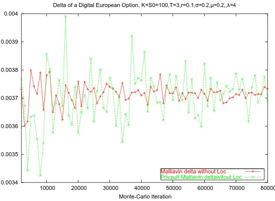
the difference between our algorithm and the one of [13] comes from the supplementary part (corresponding to the derivatives with respect to the jump amplitudes) which appears in our Malliavin weight H. In figure 2, we compare the two algorithms. Moreover, in table [1], we give the quotient between the empirical variances of the two algorithms. It turns out that the variance of the Brownian-jump algorithm (presented here) is smaller than the variance of the pure Brownian algorithm (presented in [13]). Moreover, the difference becomes more important as the number of jumps up toT increases: this happens when the maturityT is larger or when the intensity λ of the Poisson measure is larger. We conclude that more noise one uses in the integration by parts formula, better the algorithm works (there is no theoretical result in this sense, but only numerical evidence).

T \λ 1 4 8 12

1 2,15 7,27 19,88 16,43 2 1,72 12,17 22,12 36,44 3 2,94 7,15 24,30 35,58

(20)

0 0.002 0.004 0.006 0.008 0.01 0.012 0.014 0.016

10000 20000 30000 40000 50000 60000 70000 80000 Monte-Carlo Iteration

Delta of a Digital European Option, K=S0=100,T=3,r=0.1,σ=0.2,θ=0.2,λ=4

Malliavin delta without Loc Privault Malliavin delta without Loc

Finite difference,ε=0.01

Figure 1: Delta of Digital option for a Merton Process

0.0034 0.0035 0.0036 0.0037 0.0038 0.0039 0.004

Delta of a Digital European Option, K=S0=100,T=3,r=0.1,σ=0.2,µ=0.2,,λ=4

Malliavin delta without Loc Privault Malliavin deltawitout Loc

(21)

6.5 figures and comments

0 0.002 0.004 0.006 0.008 0.01 0.012 0.014 0.016

Delta of a Digital European Option, K=S0=100,T=1,r=0.1,σ=20,λ=10

Malliavin delta without Loc Finite difference,ε=0.01

Figure 3: Delta of an European digital option using Malliavin calculus and finite Difference Method. Vasicek model.

0.36 0.365 0.37 0.375 0.38 0.385 0.39 0.395 0.4

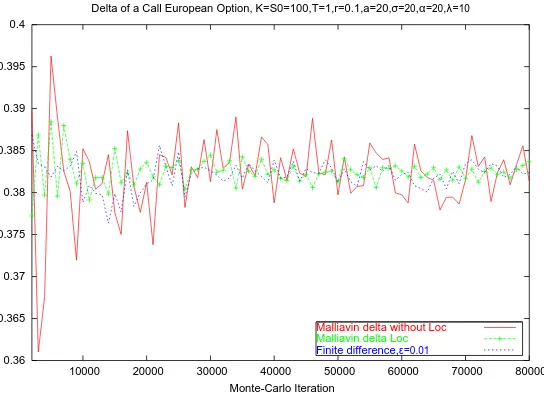
Delta of a Call European Option, K=S0=100,T=1,r=0.1,a=20,σ=20,α=20,λ=10

Malliavin delta without Loc Malliavin delta Loc

(22)

0.002 0.003 0.004 0.005 0.006 0.007 0.008 0.009 0.01 0.011

Delta of a Digital European Option, K=S0=100,T=2,r=0.1,σ=0.2

Malliavin delta

Localised Malliavin delta, a=70

Figure 5: Delta of an European digital option using Malliavin calculus and finite Difference Method. Geometrical model.

0.66 0.68 0.7 0.72 0.74 0.76 0.78

Delta of a Call European Option,Derivation wrt Amplitude, K=S0=100,T=1,r=0.1,σ=0.2

Localised Malliavin delta Malliavin delta

(23)

0.686 0.688 0.69 0.692 0.694 0.696 0.698 0.7

0 10000 20000 30000 40000 50000 60000 70000 80000 Nb MC

Delta of a Call Asian Option, K=S0=100,T=5,r=0.1,λ=1,σ=0.2

Malliavin using All Jump Amplitude Finite Difference

Figure 7: Delta of an Asian call option using localized Malliavin calculus and finite Difference Method. Geometrical model.

0.001 0.002 0.003 0.004 0.005 0.006 0.007 0.008 0.009 0.01 0.011

0 10000 20000 30000 40000 50000 60000 70000 80000 Nb MC

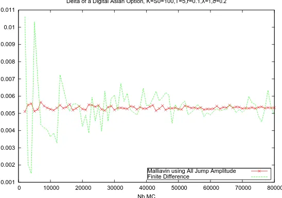
Delta of a Digital Asian Option, K=S0=100,T=5,r=0.1,λ=1,σ=0.2

Malliavin using All Jump Amplitude Finite Difference

Figure 8: Delta of an Asian digital option using localized Malliavin calculus and finite Difference Method. Geometrical model.

These figures confirm that we can numerically compute the Greeks for European options with a pure jump underlying process. We obtain numerical results similar to those in the Wiener case ([9] and [8]).

(24)

the variance of the Malliavin estimator and to make it closer to the finite difference one. On the other hand, the Malliavin estimator of a Digital option has less variance than the finite difference one (see figures 3 and 5) and so does not need to be localized: in this case, the first derivative of the payoff is a Dirac and, contrary to the finite difference method, the Malliavin calculus permits to avoid this strong discontinuity.

Finally, notice that for both call and digital options, the finite difference method requires to simulate twice more samples of the asset than the Malliavin method does : the finite difference method uses the samples starting from S₀ and those starting from S₀ +ǫ. So the Malliavin method is less time consuming.

Conclusion

In order to develop a Malliavin calculus for jump processes, we worked here on a space of simple functionals of a finite set of random variables representing the source of randomness. First, we applied the Malliavin calculus to pure jump processes, by differentiating with respect to the jump amplitudes. Second, in the case of Merton process, we used the total randomness coming from the jump amplitudes and the Brownian increments. Then, for the sensitivity analysis, we have set up (under some non degeneracy conditions) an integration by parts formula, which permits to replace the derivative of the payoff by a Malliavin weight.

The Numerical experiments show that using Malliavin approach becomes extremely efficient for a discontinuous payoff. Some specific techniques can be used to reduce the variance of the Malliavin estimator.

(25)

References

[1] F. Biagini, B. ∅ksendal, A. Sulem, and N. Wallner. An introduction to white noise and Malliavin calculus for fractional Brownian motion. To appear in Proc. Royal Soc. London., page 35 pages, 2003.

[2] K. Bichteler, J. B. Gravereaux, and J. Jacod. Malliavin calculus for processes with jumps. Gordon and Breach, 1987. MR1008471

[3] N. Bouleau. Error Calculus For Finance and Physics, The Language of Dirichlet Forms. De Gruyter, 2003. MR2079474

[4] Eric A. Carlen and ´Etienne Pardoux. Differential calculus and integration by parts on Poisson space. Kluwer ed, Stochastics, algebra and analysis in classical and quantum dynamics., pages 63–73, 1990.

[5] R. Cont and P. Tankov. Financial modelling with Jump Processes. Chapman Hall / CRC Press, 2003. MR2042661

[6] M. H. A. Davis and M. Johansson. Malliavin Monte Carlo Greeks for jump diffusions. Preprint submitted to Stochastic Processes and their Applications., 2004.

[7] B.∅ksendal. An introduction to Malliavin calculus with applications to economics. Lecture notes, Norwegian School of Economics and Business Administration, Norway, 1996.

[8] E. Fourni´e, J. M. Lasry, J. Lebouchoux, and P. L. Lions. Applications of Malliavin Calculus to Monte Carlo Methods in Finance II. Finance Stoch., 2:73–88, 2001.

[9] E. Fourni´e, J. M. Lasry, J. Lebouchoux, P. L. Lions, and N. Touzi. Applications of Malliavin calculus to Monte Carlo Methods in Finance. Finance Stoch., 5(2):201–236, 1999.

[10] Y. El Khatib and N. Privault. Computation of greeks in a market with jumps via the malliavin calculus. Finance Stoch., 8:161–179, 2004. MR2048826

[11] D. Nualart and J. Vives. Anticipative calculus for the Poisson process based on the Fock space. sem Proba. XXIV, Lect. Notes in Math., 1426:154–165, Springer (1990).MR1071538 [12] G. Di Nunno, B.∅ksendal, and F. Proske. Malliavin calculus for L´evy processes. To appear

in Proc. Royal Soc. London., Manuscript, 2003.

[13] N. Privault and V. Debelley. Sensitivity analysis of European options in the Merton model via the Malliavin calculus on the Wiener space. Preprint., 2004.