Directory UMM :Journals:Journal of Health Economics:Vol19.Issue5.Sep2000:

www.elsevier.nlrlocatereconbase

Health care expenditure in the last months of

life

Stefan Felder

a,)

, Markus Meier

b

, Horst Schmitt

a

a

Health Economics Department, Faculties of Medicine and Economics, Otto-Õon-Guericke UniÕersity

Magdeburg, Leipziger Strasse 44, 39120 Magdeburg, Germany b

Department of Economics, Socioeconomic Institute, UniÕersity of Zurich, Zurich, Switzerland

Received 12 May 1997; received in revised form 11 May 1999; accepted 6 January 2000

Abstract

Ž .

In OECD countries, a considerable share of health care expenditure HCE is spent for the care of the terminally ill. This paper derives the demand for HCE in the last 2 years of life from a model that accounts for age, mortality risk and wealth. The empirical tests are based on data of deceased members of a major Swiss sick fund. The empirical evidence

Ž .

confirms most of the hypotheses derived from the model, i.e., i HCE increases with

Ž . Ž .

closeness to death, ii for retired individuals, HCE decreases with age, and iii low-income individuals, as compared to high-income individuals, incur lower HCE in the last months of life.q_{2000 Elsevier Science B.V. All rights reserved.}

JEL classification: I12; I31; D61

Keywords: Mortality risk; Willingness to pay for survival; Demand for health care services

1. Introduction

The cost of treating the terminally ill is sometimes blamed for the steady increase in health care costs. Indeed, the so-called cost of dying is substantial. As

Ž .

Lubitz and Riley 1993 report for the United States, 30% of the total Medicare

)_{Corresponding author. Tel.:q49-391-532-8050; fax:q49-391-671-90250.}

Ž .

E-mail address: stefan.felder@medizin.uni-magdeburg.de S. Felder .

0167-6296r00r$ - see front matterq_{2000 Elsevier Science B.V. All rights reserved.}

Ž .

budget is paid out on behalf of persons in their last year of life. Spending per decedent is about seven times larger than per survivor. For Switzerland, health

Ž .

care expenditure HCE of the terminally ill is comparably high, as samples of two

Ž .

health insurance companies show cf. Zweifel et al., 1999 . Payments for persons in their last year of life constitute 22% and 18% of the total health care cost of retired persons, depending on the sample. The average ratio of per capita expendi-ture between decedents and survivors equals 5.6:1.1

Besides its size, the path of HCE in the last year of life is exceptional as well. One observes a steady increase, accentuated by a surge in the last quarter of life.

Ž .

In the study by Lubitz and Riley 1993 , 62% of all Medicare costs referring to the last year of life were incurred in the last quarter, compared to 10% in the first

Ž

quarter. In Switzerland, the difference is less accentuated 42–48% as opposed to

Ž ..

14–18%, depending on the sample cf. Zweifel et al., 1999; Table 1 .

A third characteristic of HCE in the last months of life is age dependency.

Ž .

Baker et al. 1995 reported that cost in the last 2 years of life for persons who died at 101 years of age or older was 37% of those incurred by persons who died at 70. In the Swiss samples, we found a similar pattern with respect to age and HCE in the last 2 years of life.

The present paper presents a model designed to explain these three character-istics of HCE in the last months of life. It derives the demand for health care services in the last months of life from a life-cycle model that formalises the trade-off between utility of living and utility of consumption. Section 2 deduces the willingness to pay for a change in the mortality schedule and shows how willingness to pay is affected by age, wealth and the risk of death. Section 3 presents the data and the hypotheses referring to the impact of age, closeness to death, wealth and insurance coverage on HCE. Section 4 discusses the empirical results, and Section 5 concludes.

2. The model

We assume that consumption and age are the only arguments in the utility

w Ž .x

function of a representative household. By u c t , we denote the utility of being alive at age t, given consumption c. The twice differentiable utility function u, determined up to a multiplicative factor, is positive, increasing and strictly concave. Furthermore, we assume that there is no bequest motive, and that a

1

The Swiss figures are lower compared to the US ones because Swiss hospitals are heavily subsidised by the government. For that reason, payments by the insurance companies for inpatient care

Ž .

household of age a chooses its consumption path by maximising expected residual lifetime welfare

`

yrŽtya.

EU a

Ž .

s

H

u c t

Ž .

pa

Ž .

t e d t ,

Ž .

1 a

where rG0 is the rate of time preference assumed to be equal to the interest rate.

Ž .

The conditional probability p t of surviving until age t, given that the householda

Ž .

has survived until age a, is a function of the age-specific positive death rates

Ž . q t :

t Ž . yHq s d s

p_a

Ž .

t se a .

Ž .

2

Ž . Ž . Ž .

Substituting Eq. 2 for p t in Eq. 1 shows that the forces of mortalitya increase the effective rate of time preference. The household discounts future utility more strongly because there is a positive probability that it will not survive. Suppose that there is a market for actuarially fair annuities so that the lifetime

Ž .

budget constraint can be written as cf. Yaari, 1965 :

`

yrŽtya.

waq

H

Ž

l t

Ž .

yc t

Ž .

.

pa

Ž .

t e d ts0,

Ž .

3 a

Ž .

where l t G0 is labour income at age t and w denotes non-human wealth at agea

a. With the purchase of an annuity, the household insures against the risk of

longevity and achieves an increase in welfare. The optimal consumption path follows from the optimal control problem

max EU a

Ž .

c

Ž .

subject to Eq. 3 .

The household will trade human and non-human wealth against an annuity that guarantees a fixed consumption stream until the date of death. Along the optimal

X

w Ž .x

consumption path, marginal utility u c t is equalised across periods:

X X

u c t

Ž .

su c a

Ž .

;tGa.

Ž .

4 Due to the properties of u, the optimal consumption path c is also constant in

Ž .

time. Hence, the solution c and the performance functional EU a are given by

w_aql_a

cs and EU a

Ž .

su c

Ž .

ma,

Ž .

5

m_a

respectively. Here, the discounted remaining life expectancym_aand human wealth

l_a are defined as

` `

yrŽtya. yrŽtya.

ma[

H

pa

Ž .

t e d t and la[

H

l t p

Ž .

a

Ž .

t e d t.

Ž .

6

a a

Ž . Ž .

caused by an infinitesimally small positive change dq t of the hazard rate q t .

Ž . 2

Due to Eq. 2 , we find

dpa

Ž .

t t

s ypa

Ž .

t

H

dq s d s

Ž .

-0,

Ž .

7

dq t

Ž .

a

which ensures that the probability to survive decreases. When the mortality schedule changes, the household will adjust its consumption path, and expected residual lifetime welfare will change. First, we derive for the expected marginal lifetime welfare of wealth at age a:

EEU a

Ž .

X

su ,

Ž .

8

Ew_a

Ž .

a result that is not dependent on the choice of dq t . Furthermore, we find from Ž .

Eq. 5

dc 1 dl_a dm_a

s

ž

yc

/

,

Ž .

9

dq t

Ž .

ma dq t

Ž .

dq t

Ž .

and

dEU a

Ž .

X dla u dma

su q

ž

Xyc

/

.

Ž .

10

dq t

Ž .

dq t

Ž .

u dq t

Ž .

A change in the mortality schedule affects expected lifetime welfare through

Ž . Ž .

the change in non-human wealth dlardq t and in life expectancy dmardq t ,

Ž X

.

respectively. The latter is weighted by uru yc, the consumer’s surplus from

being alive in any year with consumption level c.

The wealth equivalent of the change in lifetime welfare due to a change in the

Ž .

mortality schedule, WE a , is defined as the marginal rate of substitution between

Ž . w and q t :a

dEU a

Ž .

dl u dm

dq t

Ž .

a a

WE a

Ž .

[ _E s q

ž

Xyc

/

.

Ž .

11 EU a

Ž .

dq t

Ž .

u dq t

Ž .

Ewa

Ž . Ž

Since the utility function usu c is assumed to be normalised cf. Rosen,

. X

Ž . Ž Ž . .

1988 , we have u c - u c rc for all c)0, therefore,

dl_a

WE a

Ž .

- F0.

Ž .

12

dq t

Ž .

2 _{Ž .}

The wealth equivalent of an increase in mortality risk is negative. Households will thus have a positive willingness to pay for health care services, which restore the original mortality schedule.

For the empirical work, we are interested in three first derivatives of the wealth

Ž . Ž . Ž . Ž .

equivalent function WE a , namely, dWE arEw ,a dWE a rdq t and

Ž .

EWE arEa. The result

EWE a

Ž .

dma uuY Ec

s y X2 -0

Ž .

13

Ewa dq t

Ž .

u Ew a

Ž .

Ž .

follows from dcrdwas1rma)0 and was first derived by Jones-Lee 1976 .

Ž .

For the derivative of WE a with respect to a change in the mortality schedule, we derive

dWE a d2_{l uu}Y

dc dm u d2_m

Ž .

a a a

s ₂y X2 q

ž

Xyc

/

2.

Ž .

14

dq t

Ž .

dq t

Ž .

u dq t

Ž .

dq t

Ž .

u dq t

Ž .

Ž .

For the change of WE a , when age increases, we find

EWE a

Ž .

E dla u E dma

s q

ž

Xyc

/

.

Ž .

15

Ea Ea dq t

Ž .

u Ea dq t

Ž .

Ž Ž . Ž ..

The sign of the two derivatives Eqs. 14 and 15 cannot be determined a

Ž .

priori without fixing a special choice of the perturbation function dq t . In the

Ž .

literature, there are in principle two different approaches. In Arthur 1981 , Rosen

Ž1988 , and Shepard and Zeckhauser 1984 , the Dirac mass function. Ž . dq tŽ .[

Ž .

da t , which forces an increasing mortality risk mainly at age a, is analysed.

Ž .

We choose the change of the mortality risk in the sense of Johansson 1996 by a permanent change of the hazard rate. We set

dq t

Ž .

[q t ,

Ž .

Ž . Ž . Ž .

which might be interpreted as a parametric changeErEg of q t,g [ 1qg q t .

Additionally, we assume that we are dealing with the Gompertz’s model, i.e.,

q t

Ž .

saebt

Ž

a,b)0 .

.

For this model, we can show that3

dWE a

Ž .

-0

Ž .

16

dq t

Ž .

X

Ž .

holds, provided that waG0 and l t F0 for all tGa. Hence, if labour earnings

remain constant or fall and non-human wealth is non-negative, willingness to pay for the original mortality schedule will therefore increase when the risk of death

3

rises. This result is intuitively appealing and follows from the fact that an increase in mortality risk shortens the remaining life expectancy, which, in turn, increases the level of consumption, given that the two conditions hold. The strict concavity of the utility function then yields the desired result.

X_{Ž .}

On the other hand, if non-human life is negative or l t increases, it can not be excluded that an increase in mortality risk decreases the consumption level so that the value of life decreases. This adds another example to the list of unexpected

Ž .

results in the literature on the value of life cf. Bergstrom, 1982; Rosen, 1988 .

Ž .

The sign of dWE arda is also governed by the path of labour income. In

X

Ž .

Appendix A, Lemma 2 shows that l t F0 and the positiveness of

ŽErEa.Ždmardq tŽ ..imply the positiveness ofŽErEa.Ždlardq t . In this case, weŽ ..

therefore obtain

EWE a

Ž .

)0.

Ž .

17

Ea

Ž .

Hence, if labour earnings remain constant or fall, WE a increases with age.

Ž . Ž .

Since the value of WE a is negative, this means that the absolute value of WE a decreases with age. When a person ages, hisrher remaining life expectancy diminishes. Total consumer surplus, as well as the value of life will thus decrease with age, provided the labour income path is not decreasing. The absolute value of

Ž .

WE a may increase if labour income is growing with age. This will most likely be the case in middle age. In short, one expects that willingness to pay for life

Ž

saving follows an inverted U-shaped profile over the life cycle see also Jones-Lee

.

et al., 1985 .

Ž .

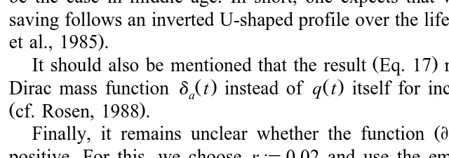
It should also be mentioned that the result Eq. 17 remains true if we use the

Ž . Ž .

Dirac mass function d_a t instead of q t itself for increasing the mortality risk Žcf. Rosen, 1988 ..

Ž .Ž Ž ..

Finally, it remains unclear whether the function ErEa dmardq t can be positive. For this, we choose r[0.02 and use the empirical data of Johansson

[image:6.595.59.379.419.532.2]

Ž . Ž . Ž .

Fig. 1. a Discounted remaining life expectancy a¨ma. b The change in remaining life

Ž Ž .Ž Ž ...

Ž1996 , where. a[0.000081 and b[0.087 were proposed. As we see, for age

Ž .

classes above 55, a positive sign can be observed see Fig. 1b .

( ( ) ( ))

Remark 1. The results Eqs. 16 and 17 are also true under less restrictiÕe assumptions on the function l. It is sufficient that the behaÕior of l is not too

X

( ) [ ] [ )

exotic, i.e., l t is positiÕe in a,T and negatiÕe in T,` where T should not be too large. The corresponding mathematics, which isÕery technical, is presented in an appendix that is aÕailable from the authors upon request.

3. Data and hypotheses

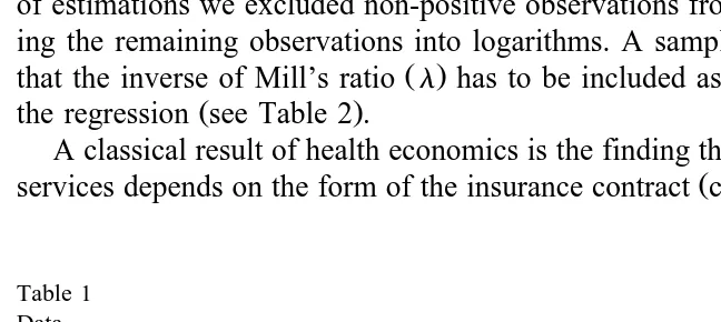
The present study is based on individual data of 415 deceased persons from a sample of more than 6000 members of a major Swiss health insurance company. The data include HCE, gender and age, as well as specifics of the insurance policy

Ž .

of the individuals. A majority of the individuals 346 were aged 65 or more at the

Ž .

time of their death see Table 1 . For simplicity, for each individual the expendi-ture records covering the last 2 years of life were aggregated into eight quarterly observations. This led to 3320 observations in the full sample and 2768 in the subsample of patients who died aged 65q, respectively. The distribution of this quarterly HCE proved to be highly skewed to the left. For this reason, for one set of estimations we excluded non-positive observations from the sample, transform-ing the remaintransform-ing observations into logarithms. A sample selection test indicated

Ž .

that the inverse of Mill’s ratio l has to be included as an additional variable in

Ž .

the regression see Table 2 .

A classical result of health economics is the finding that demand for health care

Ž .

[image:7.595.58.382.407.552.2]

services depends on the form of the insurance contract cf. Pauly, 1968 . With full

Table 1 Data

All individuals Age at death 65q

Number of indiÕiduals 415 346

Female 203 177

Male 212 169

Period of obserÕation

Cases of death 1987rI–1992rIV

Quarterly HCE 1985rI–1992rIV

Ž .

Number of quarterly HCE observed for each individual 8 8

Total number of obserÕations 3320 2768

)0 2770 2392

insurance coverage, the consumer price of medical services is zero, leading to an increase in demand compared to a situation without insurance. Usually, difficulties arise when deriving a relationship between willingness to pay and demand for health care services, since — abstracting from transaction costs — every positive willingness to pay is met when insurance companies pay the full bill. However, the patients in our sample have insurance policies that include either a franchise or a proportional co-insurance rate. These risk sharing schemes imply positive consumer prices for health care services and guarantee that persons with very low willingness to pay will have zero demand. Consequently, a negative relationship between price and demand for health care services can be postulated.

The previous section has shown that under certain conditions, willingness to pay for changing the mortality schedule increases with the risk of death. Though the data available do not give any information on the health status of the patient, and in particular do not include any diagnosis code indicating the risk of death, it seems fair to assume that health status deteriorates and the risk of death increases over the last quarters of life. Moreover, in those cases where death does not accidentally occur, one can expect patients to consider costs and benefits when deciding on health care services. This leads to

Hypothesis 1. HCE in the last months of life increases with closeness to the time

of death.

Hypotheses 2 and 3 follow from the profile of willingness to pay for change in the mortality schedule over the life cycle. When labour earnings cease to increase, willingness to pay for survival decreases with age. For retired people, willingness to pay for life-saving health care services is therefore likely to decrease with age. On the other hand, young people’s willingness to pay for survival increases with age. From that, we derive

Ž .

Hypothesis 2. HCE in the last months of life is higher for young 64y than for

Ž .

retired persons 65q .

Hypothesis 3. Within the age class 65q, HCE in the last months of life decreases with age.

Some individuals in the two samples receive government transfers targeted to reduce health insurance premiums for low-income households. Our data include information on subsidised premiums, allowing us to differentiate between low- and high-income classes and to derive

Hypothesis 4. Since willingness to pay for survival increases with wealth,

The insurance policies show different coverage with respect to inpatient care. While most patients have coverage for general hospital care, some have supple-mentary insurance that guarantees preferred treatment in the so-called private section of hospitals. Because the cost of treatment for a person receiving privi-leged treatment is higher and the hospital can charge higher fees, this gives rise to

Hypothesis 5. Supplementary hospital insurance results in higher HCE in the

terminal months of life.

In order to estimate the relationship between HCE in the last 2 years of life and the different variables mentioned in Hypotheses 1–5, the following equation was specified

HCE _{sb qb Aqb A}2_{qb SexFqb ASexFqb D qb l}

0 1 2 3 4 5 65 6

ž

log HCE

/

7 1992

qb7Subsqb8Insq

Ý

gqQuarqq

Ý

dtYeartqe.

Ž .

18

qs1 ts1986

2 _Ž

Therein A denotes calendar age in years and A the squared value of age to

. Ž

consider possible non-linearities . SexF is a dummy for sex s1, if female; s0,

.

if male . The product ASexF considers possible interactions between age and sex in the determination of HCE. D65 is again a dummy variable, taking on a value of

Ž .

unity, if a person is 65 or older s0, otherwise . lis the inverse of Mill’s ratio, capturing the impact of potential sample selection when excluding zero observa-tions. Subs is a dummy indicating that an individual health insurance premium is

Ž .

subsidised by the government s0, otherwise , Ins denotes a dummy indicating

Ž

an insurance policy providing for privileged treatment in the hospital s0,

.

otherwise , Quar a dummy taking on the value of one in quarter q before deathq

Žs0, otherwise, with qs8 serving as the benchmark , and, finally, Year is a. t

Ž

dummy taking on the value of one in year t s0, otherwise, with ts1985 as the

.

benchmark year , and e is the error term.

4. Estimation results

Ž

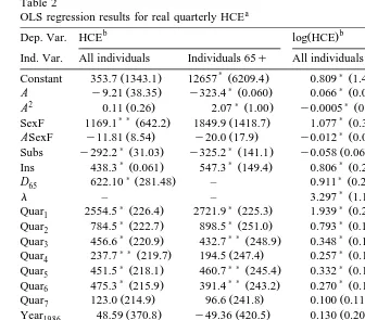
Table 2 presents the estimated coefficients and their standard errors in

.

parentheses as well as general statistics of the regressions for both the total sample and the elderly subsample, which excludes individuals aged 64 and less at their date of death. The first set of results refers to the regressions where quarterly HCE in the last 2 years of life is the dependent variable. The second regression

Ž

refers to the logarithms of HCE and implements a two-stage approach Heckman,

.

[image:10.595.47.383.67.362.2]

Table 2

OLS regression results for real quarterly HCEa

b _{Ž .}b

Dep. Var. HCE log HCE

Ind. Var. All individuals Individuals 65q All individuals Individuals 65q

) ) )

Ž . Ž . Ž . Ž .

Constant 353.7 1343.1 12657 6209.4 0.809 1.463 9.886 3.265

) )

Ž . Ž . Ž . Ž .

A y9.21 38.35 y323.4 0.060 0.066 0.026 y0.151 0.080

2 _{Ž .} )_{Ž .} )_{Ž . Ž .}

A 0.11 0.26 2.07 1.00 y0.0005 0.0002 0.0001 0.0005

) )_{Ž . Ž .} )_{Ž . Ž .}

SexF 1169.1 642.2 1849.9 1418.7 1.077 0.354 1.324 0.734

) ) )

Ž . Ž . Ž . Ž .

ASexF y11.81 8.54 y20.0 17.9 y0.012 0.005 y0.013 0.009

)_{Ž .} )_{Ž . Ž . Ž .}

Subs y292.2 31.03 y325.2 141.1 y0.058 0.067 y0.109 0.070

)_{Ž .} )_{Ž .} )_{Ž .} )_{Ž .}

Ins 438.3 0.061 547.3 149.4 0.806 0.205 0.762 0.229

)_{Ž .} )_{Ž .}

D65 622.10 281.48 – 0.911 0.275 –

)_{Ž .} )_{Ž .}

l – – 3.297 1.103 2.950 1.218

)_{Ž .} )_{Ž .} )_{Ž .} )_{Ž .}

Quar1 2554.5 226.4 2721.9 225.3 1.939 0.221 1.944 0.249

)_{Ž .} )_{Ž .} )_{Ž .} )_{Ž .}

Quar2 784.5 222.7 898.5 251.0 0.793 0.142 0.840 0.153

)_{Ž .} ) )_{Ž .} )_{Ž .} )_{Ž .}

Quar3 456.6 220.9 432.7 248.9 0.348 0.115 0.559 0.147

) )_{Ž . Ž .} )_{Ž .} ) )_{Ž .}

Quar4 237.7 219.7 194.5 247.4 0.257 0.114 0.233 0.123

)_{Ž .} ) )_{Ž .} )_{Ž .} ) )_{Ž .}

Quar5 451.5 218.1 460.7 245.4 0.332 0.114 0.312 0.122

)_{Ž .} ) )_{Ž .} )_{Ž .} ) )_{Ž .}

Quar6 475.3 215.9 391.4 243.2 0.270 0.113 0.266 0.121

Ž . Ž . Ž . Ž .

Quar7 123.0 214.9 96.6 241.8 0.100 0.113 0.107 0.122

Ž . Ž . Ž . Ž .

Year1986 48.59 370.8 y49.36 420.5 0.130 0.204 0.130 0.218

)_{Ž .} ) )_{Ž .} )_{Ž . Ž .}

Year1987 707.9 360.4 640.6 407.1 0.520 0.198 0.525 0.212

) )

Ž . Ž . Ž . Ž .

Year1988 199.0 354.6 158.5 397.7 0.313 0.195 0.334 0.208

) ) )

Ž . Ž . Ž . Ž .

Year1989 430.1 354.0 422.2 396.0 0.522 0.209 0.618 0.242

) )_{Ž .} )_{Ž .} )_{Ž .} )_{Ž .}

Year1990 629.5 350.8 681.8 392.9 0.764 0.223 0.861 0.274

)_{Ž .} )_{Ž .} )_{Ž .} )_{Ž .}

Year1991 1089.9 367.3 1208.3 412.7 0.930 0.230 1.024 0.272

)_{Ž .} )_{Ž .} )_{Ž .} )_{Ž .}

Year1992 1386.9 445.4 1597.5 506.7 0.724 0.239 0.886 0.259

2

Adj. R 0.09 0.10 0.10 0.11

F-value 16.71 16.09 15.40 15.25

N 3320 2768 2770 2392

a

Ž .

Deflated by the Swiss consumer price index 1981,100 .

b

Standard errors in parentheses.

)_{Significantly different from zero at the 99% confidence level.} ) )_{Significantly different from zero at the 95% confidence level.}

Ž .

Closeness to death Quar to Quar1 7 has a decisive effect on the level of HCE. In the sample with all individuals, expenditure in the last quarter is 2550 Swiss francs above expenditure in the benchmark quarter. In the two stage estimation, the difference in the HCE between the 1st and the 8th quarter is 578%

Ž 1.939y0.5Ž0.221.2

.4

e y1 . Moreover, the pattern of coefficients conforms very much with expectation, showing a clear increase with closeness to death. The largest expenditure surge occurs from the second last to the last quarter. Since one expects

4

For a correct interpretation of a dummy variable in semilogarithmic equations, see Kennedy

clear signs indicating near death in the last quarter of life at the latest, those results support Hypothesis 1, which is based on the reasoning that willingness to pay for life-saving health care services increases with the risk of death.

Hypotheses 2 and 3 postulate lower expenditure for the elderly and a negative correlation between age A and HCE in the subsample of individuals aged 65q. Our sample shows higher expenditure for the elderly. The coefficient is signifi-cant, contradicting Hypothesis 2. Given that we have a very small number of young decedents in the sample, it is not clear how representative this result is.5

There is evidence from other studies that the cost of dying is higher for young than

Ž .

for elderly persons Emanuel and Emanuel, 1994; Lamers and Van Vliet, 1998 . The coefficients for age show the expected signs. Age has a negative, although decreasing effect on HCE. These findings confirm Hypothesis 3. Table 2 also shows a significant effect of SexF. In the subsample, a 65-year-old woman has an HCE of 1850 francs in excess of that of a man. This differential declines to 1450 at age 85, in view of the negative coefficient of ASexF. It is interesting to connect the sign of the age coefficients with the life expectancy difference between men and women. As it is well known, life expectancy of women is higher at every age than that of men, but the difference decreases at old age. The effect of an increasing age on the willingness to pay for life is determined by the remaining

Ž .

life expectancy. Hence, we would expect that i women c.p. have a higher

Ž .

demand for life-saving health care services than men and ii the gender difference shrinks with increasing age; a pattern that is confirmed by the regression.

The parameter of the variable Subs has a negative sign, indicating that patients with subsidised health insurance premiums have lower HCE in the last 2 years of life. Since premium subsidies are paid to low-income households, this result is in line with Hypothesis 4, which postulates that willingness to pay for life increases with wealth. However, the difference is only significant in the regression, which includes zero observations, where the difference amounts to 290 and 325 Swiss francs, depending on the sample.

Ž .

Patients who have a supplementary hospital insurance policy Inss1 incur

Ž 0.806y0.5Ž0.205.2

.

significantly higher HCE e y1s119% . Given the fact that most

Ž

people die in a hospital the hospital share in total costs during the last year of life

.

amounts to about 80% in Switzerland, according to the present sample , this is not surprising. Even if hospitals were to apply the same technology to patients who have differing insurance coverage, they still have the right to charge higher fees for the treatment of insured patients who have supplementary coverage. This result clearly vindicates Hypothesis 5.

Finally, the year dummies in the regression indicate that cost increases in the health care sector exceed economy-wide inflation. In 1992, real HCE of decedents

5

Ž 0.724y0.5Ž0.239.2

.

was 2 times e s2.00 higher than in the benchmark year 1985, probably reflecting technological changes in medicine.

5. Conclusion

HCE of persons in the last months of life shows a clear increase towards death. Moreover, there is evidence that cost of dying is higher for young than for elderly

Ž .

persons Emanuel and Emanuel, 1994; Lamers and Van Vliet, 1998 . Finally,

Ž .

Baker et al. 1995 found, while studying Medicare payments, that HCE in the last 2 years of life decreases with age. All three observations can be explained by the

Ž .

theory of life saving Schelling, 1968 . Willingness to pay for survival over the life cycle is hump shaped, increasing at young ages, peaking in middle age and declining thereafter. From that one derives a willingness to pay for life-saving

Ž . Ž .

health care services to be an increasing decreasing function of age at young old ages. An increasing demand for health care services as death approaches concurs with the hypothesis that willingness to pay increases with the risk of death.

The present paper studies HCE in the last eight quarters of life of 415 members of a Swiss health insurance company who died in the period 1987–1992. The estimations show closeness to death to be a decisive factor for HCE. Regarding the difference in the cost of dying between young and retired persons, the Swiss sample shows higher cost for the elderly, contradicting the hypothesis. In the subsamples of individuals aged 65q, there is a significant decrease in cost as age increases. Furthermore, income and the extent of insurance coverage have a significant impact on HCE in the last 2 years of life. Patients with supplementary insurance for hospital treatment incur higher cost of dying than patients with average insurance coverage. Finally, low-income households spend less on health care services in the last 2 years of life than high-income households.

The high cost of dying is one reason why critics of high-tech medicine in the industrialised world ask for a rationing of health care services according to the age

Ž .

of patients cf. Callahan, 1987 . The result of the present study, namely that HCE in the last 2 years of life depends on the health insurance contract, hints at alternatives to rationing. For instance, from a coinsurance rate that increases with age according to the risk of death, a dampening effect on the ever rising health

Ž .

care cost might be expected cf. Felder, 1997 .

probability on the physicians’ decisions — a task that does not seem promising. We propose an alternative way to incorporate the supply side and argue that physicians have paternalistic preferences, i.e., that they follow rules that are socially desirable.6 The theory from which optimal physicians’ decisions under the paternalistic preference assumption can be derived is, of course, the value of life concept we have presented in Section 2.

The data used in the present study could serve as a base for further investiga-tions. From a comparison of the amount of life-saving health care services demanded at different ages, willingness to pay for survival could be derived. It would be interesting to compare the corresponding findings with existing results in literature, for instance derived from the risk premium paid in jobs with different

Ž .

death risks, respectively see Rosen and Thaler, 1975 and Viscusi, 1992 .

Acknowledgements

The paper was presented at the inaugural conference of the International Health Economics Association, Vancouver, Canada, May 19–23, 1996, and the Annual Meeting of the Verein of Socialpolitik, Kassel, September 25–27, 1996. We thank the participants as well as two anonymous referees for their helpful comments, and the Swiss National Science Foundation for financial support under grant 4032-035660.

Appendix A

Ž . Ž .

In order to complete Eqs. 16 and 17 , respectively, we must prove the following two statements.

X

( )

Lemma 1. Let l t F0 for all tGa and wa)0. Then

dWE a

Ž .

-0.

Ž .

19

dq t

Ž .

6 _{Ž .}

Cf. Detsky et al. 1981 , who studied the correlation between the predicted short-term survival probabilities of patients admitted to an intensive care unit and the expenditure for these patients. The spending was largest for patients whom physicians expected to live but did not, and for patients whom

Ž .

Ž . bt _{Ž .}

Proof. For the Gompertz’s model, i.e., q t sae , the function p t , given bya

Ž . Ž . Ž . t _{Ž .}

Eq. 2 , satisfies the differential equation p t

˙

a s ybp ta Hy`dq s d s.

There-fore, we find by integrations by parts

`

dma dpa

Ž .

t _yrŽtya. 1

s

H

e d ts

Ž

ma

Ž

q a

Ž .

qr

.

y1

.

-0.

Ž .

20

dq t

Ž .

a dq t

Ž .

b

It follows that

d2_{m q a}

qr dm

Ž .

a a

s -0.

Ž .

21

2 _{b d}

q t

Ž .

dq t

Ž .

Similarly

`

dla dpa

Ž .

t _yrŽtya.

s

H

l t e

Ž .

d t

dq t

Ž .

a dq t

Ž .

1 1 _X

s

Ž

la

Ž

q a

Ž .

qr

.

yl a

Ž .

.

y laF0,

Ž .

22

b b

where

`

X X yrŽtya.

la[

H

pa

Ž . Ž .

t l t e d t , a

which implies

2

`

dla _sq a

Ž .

qr dla _y1

H

dpa

Ž .

t _{l t e}X

Ž .

yrŽtya._{d tF0.}

Ž .

₂₃

2 _{b dq t}

Ž .

_{b dq t}

Ž .

a

dq t

Ž .

Ž . Ž .

In the next step, we show that dcrdq t is positive. Since dcrdq t is given by

1 _`dpa

Ž .

t _yrŽtya.

Ž Ž . .

Ha l t yc e d t it is sufficient to show that

ma dq t

Ž .

`dp_a

Ž .

t

yrŽtya. l t

Ž .

yc e d t)0

Ž

.

H

_{a dq t}

Ž .

Ž . t _{Ž .}

holds. Note that the functionÕ t [yH dq s d s is negative and strictly

decreas-1 a

Ž . Ž .Ž Ž . . yrŽtya. ` _{Ž .}

ing. Furthermore, we denote Õ t [p t l t yc e . Since H Õ t d ts

2 a a 2

yw , we have_a

`

Õ

Ž .

t d t-0.

H

2

Ž . Ž .

If Õ t is negative for all tg a,`, we are done. In the opposite case, there exists

2

Ž . Ž . Ž . Ž .

an sg a,` such that Õ s s0, as well as Õ t G0 for all tg a, s and

2 2

Ž . Ž .

Õ t F0 for all tg s,` . Hence,

2

`dp_a

Ž .

t `

yrŽtya.

l t

Ž .

yc e d ts Õ

Ž .

t Õ

Ž .

t d t

Ž

.

H

H

1 2

dq t

Ž .

a a

s `

s

H

Õ

Ž .

t Õ

Ž .

t d tq

H

Õ

Ž .

t Õ

Ž .

t d t

1 2 1 2

a s

s `

G

H

Õ

Ž .

s Õ

Ž .

t d tq

H

Õ

Ž .

s Õ

Ž .

t d t

1 2 1 2

a s

`

sÕ

Ž .

s

H

Õ

Ž .

t d t)0.

1 2

a

Ž .

Finally, using Eq. 14 , it follows

dWE a

Ž .

uuY dc dma

-y X2 -0,

Ž .

24

dq t

Ž .

u dq t

Ž .

dq t

Ž .

which proves the lemma. I

X

( ) ( )( ( ))

Lemma 2. Let l t F0 for all tGa and ErEa dmardq t )0. Then

E dl_a

G0.

Ea dq t

Ž .

Proof. We calculate

E dl_a

Ea dq t

Ž .

1 _X

s _b

Ž

q a

Ž .

qr

.

Ž

yl a

Ž .

q

Ž

q a

Ž .

qr

.

layla

.

qlaq a

Ž .

dl_a

s

Ž

q a

Ž .

qr

.

qlaq a

Ž .

dq t

Ž .

` q a

Ž .

yq t

Ž .

yrŽtya. s

H

ž

Ž

q a

Ž .

qr

.

ž

/

qq a

Ž . Ž .

/

l t pa

Ž .

t e d t

b

and

E dm_a 1

s

Ž

q a

Ž .

qr

.

Ž

y1q

Ž

q a

Ž .

qr

.

ma

.

qmaq a

Ž .

Ea dq t

Ž .

b dm_a

s

Ž

q a

Ž .

qr

.

qmaq a

Ž .

dq t

Ž .

` q a

Ž .

yq t

Ž .

yrŽtya. s

H

ž

Ž

q a

Ž .

qr

.

ž

/

qq a

Ž .

/

pa

Ž .

t e d t ,

b

a

Ž .Ž Ž ..

which shows that the representations of ErEa dm_ardq t and

ŽErEa.Ždl_ardq tŽ ..are similar. Following now the proof of Lemma 1 with

Õ₁

Ž .

t [l t

Ž .

and

q a

Ž .

yq t

Ž .

_yrŽtya.

Õ₂

Ž .

t [

ž

Ž

q a

Ž .

qr

.

ž

/

qq a

Ž .

/

p_a

Ž .

t e

b

gives the desired result. I

References

Arthur, W.B., 1981. The economics of risks to life. American Economic Review 71, 54–64. Baker, C., Beebe, J., Lubitz, J., 1995. Longevity and medicare expenditure. The New England Journal

Ž .

of Medicine 332 15 , 999–1003.

Bergstrom, T.C., 1982. When is a man’s life worth more than his human capital? In: Jones-Lee, M.W.

ŽEd. , Valuation of Life and Safety. North-Holland, Amsterdam, pp. 3–26..

Callahan, D., 1987. Setting Limits: Medicare Goals in an Aging Society. Simon and Schuster, New York.

Detsky, A., Mulley, A.G., Stricker, S.C., Thibault, G.E., 1981. Prognosis, survival, and the expenditure of hospital resources for patients in an intensive care unit. New England Journal of Medicine 305

Ž17 , 667–672..

Emanuel, E.J., Emanuel, L.L., 1994. The economics of dying: the illusion of cost savings at the end of

Ž .

life. The New England Journal of Medicine 330 8 , 540–544.

Ž .

Felder, S., 1997. Costs of dying: alternatives to rationing. Health Policy 39 2 , 167–176. Heckman, J.J., 1989. Sample selection bias as a specification error. Econometrica 47, 153–160. Jones-Lee, M.-W., 1976. The Value of Life: An Economic Analysis. University of Chicago Press,

Chicago.

Jones-Lee, M.-W., Hammerton, M., Philips, P.R., 1985. The value of safety: results of a national sample survey. Economic Journal 95, 49–72.

Johansson, P.-O., 1996. On the value of changes in life expectancy. Journal of Health Economics 15, 105–113.

Kennedy, P.E., 1981. Estimation with correctly interpreted dummy variables in semilogarithmic equations. Economic Review 71, 802.

Lubitz, J.B., Riley, G.F., 1993. Trends in medicare payments in the last year of life. The New England

Ž .

Journal of Medicine 328 15 , 1092–1096.

Newhouse, J., 1992. Medical care costs: how much welfare loss? Journal of Economic Perspectives 6

Ž .3 , 3–21.

Pauly, M.V., 1968. The economics of moral hazard: comment. American Economic Review 58, 531–537.

Rosen, S., 1988. The value of changes in life expectancy. Journal of Risk and Uncertainty 1, 285–304. Rosen, S., Thaler, R., 1975. The value of saving a life: evidence from the labor markets. In: Terleckyi,

Ž .

N. Ed. , The Measurement of Economic and Social Performance. National Bureau of Economic Research, New York.

Ž .

Schelling, T.C., 1968. The life you save may be your own. In: Chase, S.B. Ed. , Problems in Public Expenditure Analysis. Brookings Institution, Washington, DC.

Shepard, D.S., Zeckhauser, R.S., 1984. Survival versus consumption. Management Science 30, 423–439.

Viscusi, W.K., 1992. Fatal Tradeoffs: Public and Private Responsibilities for Risk. Oxford Univ. Press, New York.

Yaari, M., 1965. The uncertain lifetime, life insurance and the theory of the consumer. Review of Economic Studies 32, 137–150.

Zweifel, P., Felder, S., Meier, M., 1999. Ageing of population and health care expenditure: a red

Ž .