www.elsevier.nlrlocatereconbase
Adaptation and scale of reference bias in
self-assessments of quality of life
Wim Groot
a,b,)a
Department of Health Sciences, Maastricht UniÕersity, P.O. Box 616,
6200 MD Maastricht, Netherlands b
Research Centre on Schooling, Labour Market and Economic DeÕelopment, Department of
Economics, UniÕersity of Amsterdam, Amsterdam, Netherlands
Received 8 September 1998; received in revised form 8 July 1999; accepted 15 November 1999
Abstract
Adaptation behaviour and different scales of reference can bias self-assessments of well-being by individuals. In this paper, we analyse the impact of these biases on a subjective measure of the quality of health and on the QALY weights derived from this health measure. It is found that the scale of reference of the subjective health measure changes with age. Accounting for adaptation and scale of reference bias lowers most of the QALY weights for health problems and disabilities. q2000 Elsevier Science B.V. All
rights reserved.
JEL classification: I1
Keywords: QALY; Adaptation; Subjective health
1. Introduction
It is frequently observed that people have a remarkable ability to adapt to discomfort and illness. Chronically ill patients generally report levels of quality of life that are much higher than one would expect given their condition. For
)Department of Health Sciences, Maastricht University, PO Box 616, 6200 MD Maastricht,
Netherlands. Tel.:q31-43-388-1588r1727; fax:q31-43-367-0960; e-mail: [email protected]
0167-6296r00r$ - see front matterq2000 Elsevier Science B.V. All rights reserved.
Ž .
Ž .
example, in Adang 1997 , type I diabetes and end-stage renal disease patients are asked to rate their quality of life on a 10-point scale before and after they receive a combined pancreas–kidney transplantation. These are people who are seriously ill, suffer a great deal of discomfort and are highly restricted in their activities. Before the transplantation, the average quality of life is rated at 5.5. After a successful transplantation this increases to 7. If, however, after the transplantation these patients are asked retrospectively about their pre-transplant quality of life, this is rated at 3.3. What this indicates is that patients highly adapt to their situation. This
Ž
is just one example that shows that patients adapt to their situation for other
.
examples, see Adang, 1997 and Heyink, 1993 .
Ž .
Adaptation is defined by Heyink 1993 as ‘‘ . . . an intrapsychic process in which past, present, and future situations and circumstances are given such cognitive and emotional meaning that an acceptable level of well-being is
Ž . 1
achieved’’ Heyink, 1993, p. 1332 . Adaptation is used by people to recover psychologically from a setback. Adaptation is related to coping behaviour — i.e., behaviour aimed at reducing or eliminating psychological distress. The difference between coping and adaptation is that coping theory does not predict whether the outcome of the process will be positive or negative, while adaptation implies
Ž .
recovery and thus a positive outcome of the process Heyink, 1993 . In the
Ž .
adaptation model of well-being of Chamberlain and Zika 1992 it is argued that
Ž
well-being is stable in the absence of situational change such as the occurrence of
.
an illness or disability , sensitive to change when situational change occurs, and adaptive to occurrence of change.
Adaptation may not be the only explanation for the frequent finding that people with health problems or handicaps report higher levels of well-being than ex-pected. An alternative explanation might be that questions on well-being are answered relative to a certain reference group. If you are asked about your well-being you do so by comparing yourself to people in a similar situation as
Ž .
yourself friends, relative, people of your age, people with similar education, etc. ,
Ž
or by comparing the sources of your well-being with those of others people with more health problems than yourself, people without a job, people with a low
.
income, etc. . The finding that patients with diabetes report relatively high levels of well-being may be because they compare themselves to other patients in a similar physical condition, or they may compare themselves to the situation they had expected themselves to be in at that stage of their disease. In short, questions
1
The psychological notions of coping and adaptations have their counterparts in economic theory
Ž
also. An economic interpretation adaptation can be found in the notion that utility is relative see, Groot
.
and Maassen van den Brink, 1999 for an example . Some economists have tried to incorporate notions
Ž .
of adaptation and habit formation in economic models. For example, Alessie and Kapteyn 1991 and
Ž .
on subjective well-being do not have the same meaning to everyone. Subjective measure of well-being do not have a natural reference point. Rather, the reference point of well-being is determined by individual specific situations and character-istics.
Empirically, it may not be possible to distinguish between adaptation and differences in the scale of reference. In a sense, adaptation may be a specific form of changes in the scale of reference. Once you have health problems or a disability your point of reference changes to adapt to the new situation.
As shown by the example of type I diabetes and end-stage renal disease patients, adaptation behaviour and different scales of reference between individu-als may bias the answers to survey questions on subjective well-being or subjec-tive quality of life. Subjecsubjec-tive measures of the quality of life are an essential part
Ž .
of Quality Adjusted Life Years Studies QALYs . Subjective measures of the quality of life are used as QALY weights to diseases. Three different ways to measure QALY weights can be distinguished.
The first is to ask patients to judge their quality of life. Either patients can be
Ž
asked to evaluate their quality of life before and after a medical intervention as
.
was done in Adang, 1997 , or the quality of life of patients can be compared to the quality of life of healthy people, or patients can be asked to judge their quality of life with the disease and in the hypothetical situation that they are healthy.
The second method is to ask informed experts — for example doctors — about the quality of life of people with a certain disease.
The third method is based on questioning a random sample of the entire population. They are either asked about the quality of their own life and about their health status, and then the quality of life of people with health impairments can be compared with that of healthy people. Or, they are asked hypothetically about the quality of their life with a certain disease or handicap. A difference with the other methods is that in this method QALY are usually defined in terms of diseases reported by the population, rather than in terms of diseases diagnosed by a medical expert.
Of these three methods, the second one can be thought to be free from adaptation, as it is unlikely that informed experts adapt to the diseases of the people they are asked to evaluate. However, almost by definition, this method suffers from problems in the scale of reference. The scale of reference of an informed expert is not identical to that of the patient. Further, if medical experts base their evaluation of the quality of life of patients on their own experience with these patients, adaptation may bias the responses of medical experts through the adaptation of patients to their situation.
Ž
the QALY analysis of a medical treatment because they want insurance
compa-.
nies to fund the treatment , they may have an incentive to underestimate the quality of life of patients before the treatment and to overestimate the quality of life after the medical intervention.
The US Panel on Cost-Effectiveness in Health and Medicine that was set up to
Ž
provide guidelines for QALY research favours using the third method see Gold et
.
al., 1996 . The Panel recommends using community based weights for the quality of life that should be collected from a representative sample of the general population.
Ž .
Recently, Cutler and Richardson 1997; 1998 have used information on self-reported quality of health measure from a representative sample of the US population to calculate QALY weights of a wide range of different diseases.2
Ž .
Cutler and Richardson 1997; 1998 use these QALY weights to determine the increase in the value of health between 1970 and 1990. They calculate that health improved by US$100,000–US$200,000 per person between 1970 and 1990. This increase in the value of health is the outcome of two opposing trends. On the one hand longevity has improved. On the other hand, the prevalence of most diseases and handicaps is increasing. The reason for these opposing trends is that more and more diseases that in the past were fatal are not so anymore. This has increased life expectancy. Instead, many of these formerly fatal diseases have become chronic conditions. This is why the prevalence of these diseases has increased. Because of the increase in the prevalence of these diseases and handicaps, more people now have to adapt to limitations on their health condition. Adaptation has become more widespread as the prevalence of the diseases has increased. The wider prevalence of adaptation among people with diseases or handicaps will
oÕerestimate the increase in the value of health. This is noted by Cutler and
Ž .
Richardson 1998 when they discuss that the quality of life for each disease or handicap has improved over time and that people report themselves in less worse
Ž .
health than they did in the past Cutler and Richardson, 1998, p. 98 .
Ž .
The results in Cutler and Richardson 1997; 1998 probably also suffer from scale of reference bias. This is clear from their finding that the QALY weight for women in 1980 increases at very old age. They ascribe this finding to age-norm-ing. Respondents are explicitly asked to take people of their own age into account
Ž
when answering the subjective health question ‘‘How would you rate your health
.
as compared with individuals your age?’’ . In this way, older respondents are invited to use a different scale of reference than younger people.
2
Self-assessments of the quality of life or health are not only widely used in QALY and cost–benefit studies in health care, but in other areas — such as studies on the effects of health on
Ž
wages, labor supply and retirement decisions — as well see, for example, Anderson and Burkhauser, 1985; Bazzoli, 1985; Bound, 1991; Chirikos and Nestel, 1984; Dwyer and Mitchell, 1998; Haveman et
.
Unfortunately, the psychological literature does not provide a formal treatment of the notions of adaptation and scale of reference bias. Here, in this paper, we assume that adaptation and scale of reference bias occur in the transformation of the ‘true’ health state into the ‘reported’ health state. We assume that people who are in same health states can perceive their situation differently — depending on the reference group with which they compare themselves — and that these differences in perception may lead to differences in the response to a question on the assessment of their health status. So, a health condition that is assessed as ‘good’ by one person, can be perceived as only fair by another. If we observe that the same health status gives rise to different answers on a quality of health question, we may also observe the opposite, i.e., that people in different health states give similar assessments of their health situation. For example, someone with an objective handicap or disease may have adapted to the situation and evaluate hisrher quality of life at the same rate as someone without this handicap or disease.
So the first condition under which the procedure proposed in this paper is appropriate is that scale of reference bias or adaptation occurs in the translation of the true health status into the response to a question on the evaluation of this health status. The second condition is that the discrepancy between the ‘true’ and the reported health status is related to observable characteristics such as age, gender and the prevalence of health problems or disabilities. A limitation of this procedure is that it does not correct for adaptation and scale of reference bias generated by unobservable or individual specific characteristics. To correct for this would call for a longitudinal approach.
In this paper, we use these notions to formulate a method to purge self-reported quality of life measures from adaptation and scale of reference bias. In this method, we allow for the underlying distribution of health to depend on the health status and on other individual characteristics of individuals.
This method of correcting for adaptation and scale of reference bias is particularly useful for studies in which QALY weights are derived from a cross-section of people with and without health problems and disabilities, i.e., from national samples on the quality of life and health status of the population. In this paper, we use data from a large longitudinal sample of the British Population, the British Household Panel Survey 1995. QALY weights are derived from the following self-assessment of the overall-health quality of life question that was included in the survey: ‘‘Compared to people of your own age, would you say that your health has on the whole been: excellent, good, fair, poor or very poor?’’. This
Ž
quality of life variable is identical to the one used by Cutler and Richardson 1997;
.
1998 in their analysis of QALY. Like them, we use a representative sample of the population to derive QALY weights from the effects of the actual health status of an individual on hisrher subjective health.
other techniques, such as the standard gamble and the time trade-off methods. In
Ž .
Fryback et al. 1993 , it is shown that the scores on this self-assessed overall quality of health correlate highly with the scores of other quality of life indicators that are frequently used in QALY analysis, such as the time trade-off assessment, the quality of well-being index and the outcomes of a general health perception questionnaire.
The outline of this paper is as follows. In Section 2, we describe the empirical model to derive QALY weights from self-assessments of health status. We further show how we can correct QALY weights for adaptation and scale of reference bias. The data used in the empirical analysis are described in Section 3. The results are presented in Section 4. Section 5 concludes.
2. The quality of health model
In modelling the quality of life, we follow the same procedure as Cutler and
Ž .
Richardson 1997; 1998 . We build on their model by allowing for preference drift and adaptation to the health condition in the self-reported quality of health measure.
The starting point of the model is the concept of‘‘health capital’’as introduced
Ž . Ž .
by Grossman 1972 . The value of Health Capital HC at year t is defined as:
` E H
w
x
t tqk HCtsV
Ý
k1qr
Ž
.
ks0where V is the value of a year in perfect health, r is the real discount rate and Ht
is the quality of life in year t.
In the empirical modelling of the quality of life, three concepts are distin-guished. The first is the true quality of health HU. The true quality of health is a latent variable that cannot be observed directly. What we observe are an objective measure of the health status of the individual, denoted by Ho, and a subjective measure of the quality of health, Hs. The objective health measure refers to the prevalence of a number of illnesses and handicaps among the respondents in our sample. H8refers to a vector of dummy variables on illnesses and handicaps. The subjective measure of health, Hs, is measured by the response to the survey question ‘‘Compared to people of your own age, would you say that your health
Ž . Ž . Ž . Ž . Ž .
The latent health variable is assumed to be related to the objective health measure and to some other individual characteristics in the following way:
HUsb0qHob1qXb2qe
where X is a vector of individual characteristics,b are vectors of coefficients and e is a standard normal distributed random term capturing unmeasured and unmeasurable effects on the true health status.
The observed health status Hs is a categorical ordered response variable. The
observed health variable is assumed to be related to the latent variable in the following way:
Hssilciy1-HUFc ,i is0, . . . , n
Ž
where n is the number of response categories i.e., n ranges from 1 to 5 for our
.
subjective health measure and c are threshold levels. It is further assumed thati
c0s`, c1s0 and cns`. We specify the remaining ny2 threshold levels as:
cisdi for is2, . . . , ny1
where d is a coefficient to be estimated. This is the specification of the
Ž .
well-known ordered probit model McKelvey and Zavoina, 1975 .
Ž .
We follow Cutler and Richardson 1997 in calculating QALY weights from the estimates of the b1 coefficients. Let b1 i be the coefficient for disease i from the set of reported diseases Ho. As the b coefficients are not scaled and can range
from ` to y`, the b1 coefficients need to be normalised to produce a QALY
Ž .
weight. Following Cutler and Richardson 1997 we normalise by dividing them by the difference between the borderline between excellent health and that of a very poor health. Here, it is assumed that an excellent health corresponds to a near perfect health and a very poor health corresponds to near death. The QALYs are defined as:
b1 i
QALYis1y d4yd1
As for identification, c1sd1s0, the QALY for disease i becomes:
b1 i
QALYis1y d4
Not only the levels of the QALY weights are of interest, we also like to know whether the QALYs are statistically significant. We therefore calculate the stan-dard error of b1 ird4. As both b1 i and d4 are normally distributed, the
standard-Ž .
moments, we use a Taylor approximation. Let Ex1sb1 i, Var x1ss1, Ex2sd4, Var x2ss2 and zsb1 ird4. The approximation to the first-order moment then is:
b1 i s1 2b1 is2
Ezs q q 3
d4 d4 d4
The second-order moment is given by:
b2 2s 6b s
1 i 1 1 i 2 2
Ez s 2 q 2 q 4 d4 d4 d4
2 Ž .2
The standard error of z is then equal to the square root of Ez y Ez .
The threshold levels c indicate the location of the n response categories in the underlying distribution of the quality of health. The higher the level of c, the greater the distance between the response category and the normalised response
Ž .
category represented by c1s0 . Similarly, the greater the difference between two threshold levels, the greater the distance between two response categories.
As was noted in Section 1, we assume that scale of reference bias and adaption occur in the translation of the ‘true’ health status — HU — into the ‘reported’ health status, Hs. With adaptation, people with an objective health impairment
report relatively higher levels of subjective health than people with no objective illness or handicap. If an illness or handicap leads to adaptation, we expect the difference between two response categories to be smaller for people with an illness or handicap than for people who do not have this illness or handicap. That is, for people who are ill, the difference between, for example, a poor health and a fair health, becomes smaller than for people who are not ill. Or, stated otherwise, in a similar condition someone who has adapted to hisrher health problems reports hisrher health to be good, whereas someone without health problems who has not adapted would — if faced with similar health problems — describe it as only fair. Consequently, the threshold levels for the ordered response categories are expected to depend on the objective health status measure.
Differences between respondents in the scale of reference used in answering the subjective health question may have the same effect. The subjective health measure used in this paper contains at least one obvious factor that leads to differences in the scale of reference: age. People are explicitly asked to compare their health status to people of their own age. Obviously a good health for a eighty year old means something entirely different than a good health for someone who is 20 years old.
We allow for the possibility that the adaptation and scale of reference effects not only depend on the objective health status, but on other individual character-istics as well. We therefore specify the threshold levels as:
We can now rewrite the definition of the subjective health measure Hs as:
Hssi
ldiy1qHoaiy1qXgiy1yb0yHob1yXb2
-eFdiqHoaiqXgiyb0yHob1yXb2
If a-0 org-0, the difference between two response categories is smaller for people with an objective health impairment or for people with a certain character-istics. This can be interpreted as adaptation or a different scale of reference on the part of individuals with this condition or characteristic.
We can now distinguish between two types of QALY weights. In the first we ignore the response shift because of the health status Ho and the individual
characteristics X. The QALY weight for disease i is then identical to the one described above, i.e., 1yb1 ird4. In the extended model, this is the adaptation and scale of reference bias corrected QALY weight. If we do not account for response shifts because of adaptation and differences in the scale of reference the QALY weight becomes:
b1 i
QALYis1y
d4qa4 i
3. Data and descriptive analysis
The data are taken from the 1995 wave of the British Household Panel Survey
ŽBHPS, 1995 . Details about this survey can be found in Taylor 1992 . The. Ž .
sample includes all individuals over the age of 15. After eliminating a small number of observations with missing values on the self-reported health status and on the health condition variables, 9462 observations could be used in the analysis. As was already mentioned, the subjective health measure Hs is defined by the
response to the survey question ‘‘Compared to people of your own age, would you
Ž . Ž . Ž . Ž .
say that your health has on the whole been: 1 excellent, 2 good, 3 fair, 4
Ž .
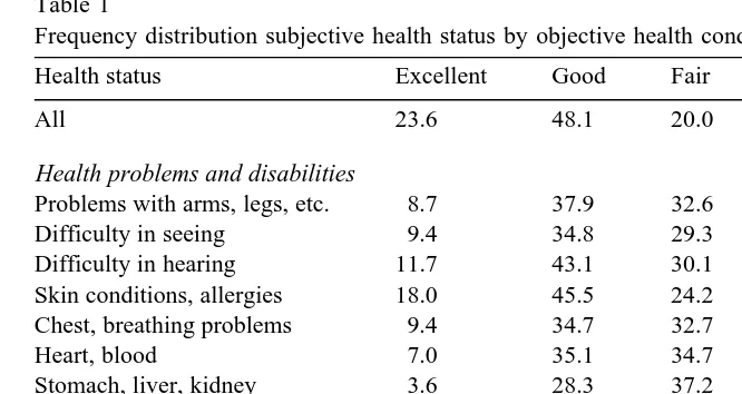
poor or 5 very poor?’’. Table 1 gives the frequency distribution of this subjective health measure. Less than a quarter of the respondents consider themselves in excellent health, while another 48% describe their health as good. A little over 8%
Ž .
are in very poor health. The remaining 20% perceive their health as fair. For the objective health measure Ho, the response to the following survey question is used: ‘‘Do you have any of the health problems or disabilities listed on
Ž .
this card? exclude temporary conditions ’’. Respondents are shown a card with a list of conditions:
–Problems or disability connected with: arms, legs, hands, feet, back, or neck
Žincluding arthritis and rheumatism ;.
Ž .
Table 1
Ž .
Frequency distribution subjective health status by objective health condition %
Health status Excellent Good Fair Poor Very poor
All 23.6 48.1 20.0 6.7 1.7
Health problems and disabilities
Problems with arms, legs, etc. 8.7 37.9 32.6 16.1 4.7
Difficulty in seeing 9.4 34.8 29.3 18.8 7.7
Difficulty in hearing 11.7 43.1 30.1 11.9 3.2
Skin conditions, allergies 18.0 45.5 24.2 10.6 1.7
Chest, breathing problems 9.4 34.7 32.7 17.6 5.6
Heart, blood 7.0 35.1 34.7 17.9 5.4
Stomach, liver, kidney 3.6 28.3 37.2 21.6 9.4
Diabetes 6.4 32.5 35.0 19.2 6.9
Nerves, anxiety, depression 4.4 25.2 36.4 24.7 9.4
Alcohol, drugs 6.3 31.3 18.8 37.5 6.3
Epilepsy 10.5 39.5 32.9 13.2 3.9
Migraine, chronic headaches 13.4 44.1 27.1 11.4 4.1
Other 5.5 31.1 33.3 20.4 9.6
–Skin conditionsrallergies;
–Chestrbreathing problems, asthma, bronchitis; –Heartrblood pressure or blood circulation problems; –Stomachrliverrkidneys or digestive problems; –Diabetes;
–Anxiety, depression or bad nerves; –Alcohol- or drug-related problems; –Epilepsy;
–Migraine or frequent headaches; –Other health problems.
The categorisation of the health problems and disabilities on this list is fairly broad. For example, heart and blood pressure problems includes both people with high blood pressure and patients with severe cardiovascular diseases. This broad categorisation may have an effect on the estimation of the QALY weights and on the impact of adaptation on these weights. A more detailed classification of health problems and disabilities would, however, have required a much larger sample size in order to obtain sufficiently large cell sizes.
Table 1 presents the frequency distribution of the subjective health evaluation by health problem and disability. For people with health problems or disabilities, subjective health status is lower than average. Alcohol and drugs problems appear to have the most detrimental effect on health. Among the people with alcohol or
Ž .
drug problems 44% report to be in a very poor health. Anxiety and depression also seems to have a highly negative effect on health: 34% of the people who
Ž .
suffer from anxiety or depression find themselves in a very poor health. Third on the list of health impediments are problems with stomach, liver and kidneys: 31%
Ž .
of the people who suffer from this are in very poor health.
4. Estimation results
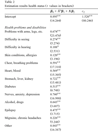
The parameter estimates of the ordered probit model are found in Table 2. As the subjective health measure runs from excellent to very poor a positive sign of the coefficient indicates that the variable lowers the health status, while a negative coefficient indicates that an increase in that variable will improve health. All objective health problems and disabilities lower the health status significantly. If we look at the effects of the other control variable, then it is found that years of education improve the health status. This finding is in line with the human capital interpretation of health, which claims that higher educated workers are able to invest more in their health. The negative coefficient for men indicates that women
Ž .
are subjectively less healthy than men.
The age effect contradicts our expectations. The sign of the coefficient indicates that older people are in better health than younger people. One explanation for this finding is the age-norming in the survey question about subjective health. In the survey people are asked to evaluate their health status compared to other people of their age. This can bias the age coefficient downward and may explain why self-reported health increases with age. Age-norming is an example of the scale of reference effect. An alternative explanation, however, is that adaptation behaviour is more prevalent among older people than among the young. Older people may have become more accustomed and have had more time to adapt to their health impairments. Both the age-norming and the adaptation explanation imply that older people have answered the question on subjective health differently from younger people. The age-norming explanation says that this question is answered relative to a reference group of people who are of the same age as the respondent. The adaptation explanation says older people have adapted themselves more to their reduced health status. In both cases we may expect the age coefficient to reverse signs if we allow for adaptation effects.
Table 2
Ž .
Estimation results health status t values in brackets
o Problems with arms, legs, etc. 0.674
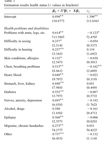
Table 3
Ž .
Estimation results health status t values in brackets
o
Problems with arms, legs, etc. 0.614 y0.123 y0.078 0.107
Ž13.580. Ž2.470. Ž1.259. Ž1.083.
U
Difficulty in seeing 0.237 y0.054 y0.111 y0.082
Ž2.514. Ž0.537. Ž0.961. Ž0.560.
UU UU U
Difficulty in hearing 0.237 0.134 0.269 0.326
Ž3.343. Ž1.692. Ž2.908. Ž2.461.
U U
Skin conditions, allergies 0.132 y0.030 0.001 0.376
Ž2.547. Ž0.501. Ž0.014. Ž2.342.
UU UU
Chest, breathing problems 0.515 y0.162 y0.097 0.046
Ž8.861. Ž2.609. Ž1.319. Ž0.450.
UU U UU
Heart, blood 0.648 y0.023 0.170 0.399
Ž9.707. Ž0.319. Ž2.058. Ž3.699.
UU U
Stomach, liver, kidney 0.880 0.051 0.249 0.272
Ž7.988. Ž0.449. Ž2.030. Ž1.906.
UU
Diabetes 0.552 y0.087 0.073 0.195
Ž3.797. Ž0.573. Ž0.411. Ž0.884.
UU
Nerves, anxiety, depression 0.691 y0.182 y0.080 y0.002
Ž6.858. Ž1.762. Ž0.711. Ž0.012.
Alcohol, drugs 0.580 y0.161 y0.470 0.745
Ž1.856. Ž0.471. Ž1.238. Ž1.158.
UU
Epilepsy 0.566 y0.006 0.244 0.310
Ž2.557. Ž0.028. Ž0.844. Ž0.855.
UU
Migraine, chronic headaches 0.273 0.031 0.079 0.062
Ž4.277. Ž0.422. Ž0.876. Ž0.438.
Years of education y0.030 0.016 y0.007 y0.001
Ž5.451. Ž2.283. Ž0.744. Ž0.041.
Number of children 0.001 y0.030 y0.063 y0.127
between a poor health and a very poor health is reduced by age: for older people, the difference between a poor health and a very poor health is smaller than for younger people. On the other hand, the gap between a good health and a fair
Ž .
widens with age this coefficient is significant at the 10% level only, however . Table 3 further shows that the difference between a good and fair health and between a fair and poor health is smaller for men than for women. This implies that where men say their health is fair, women would rather say their health is good. Where men say their health is poor, women tend to say their health is fair. This difference in the scale of reference between men and women may have something to do with different expectations men and women have about their health. It may also have something to do with differences in life expectancy between men and women. Especially at older ages, the age specific mortality rate of men is higher than for women. If men look at other men of their age they observe that mortality among men is higher than among women. This may lower their assessment of their own life expectancy and thus of their health status.
The gap between reporting a fair health and a poor health and that between a poor and a very poor health declines with the number of children. Where people with children report their health to be poor, people who are childless are more prone to say it is fair.
For the calculation of the QALY weights, it is of interest to know which of the health problems and disabilities shift the cut-off between a poor and a very poor health. The coefficients show that three health conditions significantly increase the gap between a poor and a very poor health: having difficulty in hearing, skin conditions and allergies and heartrblood pressure or blood circulation problems. This is consistent with adaptation behaviour. People with hearing difficulties, skin conditions or allergies, or heart and blood problems are inclined to say their health is poor when others will say their health is very poor.
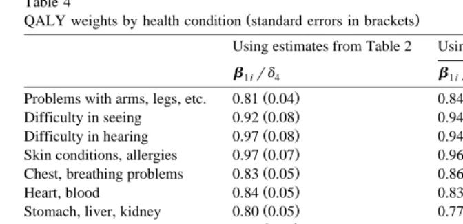
From the coefficients in Tables 2 and 3, we calculated the QALY weights for the various health problems and disabilities. These QALY weights and their standard errors are found in Table 4. Three estimates of QALY weights are presented. The figures in the first column of Table 4 are based on the estimates of the standard ordered probit model. These estimates are best comparable to those in
Ž .
Cutler and Richardson 1997; 1998 . From the coefficients in Table 3 we calculated two sets of weights: one in a similar way as those taken from the
Ž
standard ordered probit, i.e., using only the intercept terms for scaling second
.
column of Table 4 , and one using both the intercept term and the scaling
Ž
coefficient for the health problem or disability concerned third column of Table
.
Table 4
Ž .
QALY weights by health condition standard errors in brackets
Using estimates from Table 2 Using estimates from Table 3
Ž .
b1 ird4 b1 ird4 b1 ird4qa4 i
Ž . Ž . Ž .
Problems with arms, legs, etc. 0.81 0.04 0.84 0.07 0.84 0.07
Ž . Ž . Ž .
Difficulty in seeing 0.92 0.08 0.94 0.11 0.96 0.11
Ž . Ž . Ž .
Difficulty in hearing 0.97 0.08 0.94 0.09 0.96 0.09
Ž . Ž . Ž .
Skin conditions, allergies 0.97 0.07 0.96 0.08 0.97 0.08
Ž . Ž . Ž .
Chest, breathing problems 0.83 0.05 0.86 0.08 0.86 0.08
Ž . Ž . Ž .
Heart, blood 0.84 0.05 0.83 0.08 0.84 0.07
Ž . Ž . Ž .
Stomach, liver, kidney 0.80 0.05 0.77 0.06 0.78 0.05
Ž . Ž . Ž .
Diabetes 0.86 0.08 0.85 0.10 0.86 0.10
Ž . Ž . Ž .
Nerves, anxiety, depression 0.79 0.05 0.82 0.08 0.82 0.08
Ž . Ž . Ž .
Alcohol, drugs 0.82 0.09 0.85 0.12 0.87 0.10
Ž . Ž . Ž .
Epilepsy 0.87 0.10 0.85 0.11 0.86 0.11
Ž . Ž . Ž .
Migraine, chronic headaches 0.94 0.07 0.93 0.09 0.93 0.09
Ž . Ž . Ž .
Other 0.76 0.04 0.80 0.08 0.80 0.08
To the extent that the QALY weights can be compared to findings elsewhere, most of them are of similar size. A look at the results in the first column shows that the QALY weight for difficulty seeing is 0.92 and for difficulty hearing 0.97.
Ž .
Cutler and Richardson 1997 calculate QALY weights for various vision impair-ments between 0.87 and 0.97 and hearing impairimpair-ments of 0.93. For chest, breathing problems, asthma and bronchitis the weight is 0.83, whereas the weights
Ž .
for various respiratory problems in Cutler and Richardson 1997 are between 0.74 and 0.93. The standard errors in Table 4 indicate that the QALY weights for difficulties in hearing and seeing are not statistically different from 1.
For heart and blood pressure problems, the QALY weight is 0.84. Cutler and Richardson calculate weights for circulatory problems that are between 0.74 and
Ž .
0.86, while Stinnett et al. 1996 calculate QALY weights according to the presence or absence of angina and congestive heart failure that are between 0.74 and 0.90. Both the QALY for breathing problems and for heart and blood pressure problems are statistically significant from 1.
Only the QALY weight for diabetes differs from that in Cutler and Richardson
Ž1997 . They find a QALY weight for diabetes of 0.66, while we find a weight of.
Ž .
0.86. In a recent study, Douzdjian et al. 1998 find confidence intervals for QALY weights for diabetes to be between 0.4 and 0.8.
broad groups that mostly include both minor and major health impairments. A more detailed classification of health problems may result in larger adaptation and scale of reference effects for more severe health impairments.
5. Conclusion
Through their effects on QALY weights, adaptation and scale of reference bias
Ž
may affect conclusions about the cost-effectiveness of medical interventions see
.
Adang, 1997 for an example . In this paper, we have shown how we can correct for adaptation and scale of reference bias in self-assessments of well-being of individuals. It was found that if people are asked about the quality of their health status compared to others of their age, the response suffers from age-norming: older people appear to be subjectively healthier than younger people. By allowing the cut-off points between the response categories to depend on age, results are purged from this form of scale of reference bias.
For the broad categories of health problems and disabilities distinguished in this paper, correcting for adaptation and scale of reference bias reduces the value of most of the QALY weights somewhat. The relatively high QALY weights found in this paper suggest that intra-disease values dominate the inter-disease ones. Further, not all QALY weights calculated in this paper proved to be statistically different from 1. Therefore, more detailed information about health impairments is required to establish QALY weights from population based surveys and to determine the impact of adaptation and scale of reference bias on QALY weights for specific diseases and disabilities. We consider this to be a major topic for further research.
Acknowledgements
I would like to thank two anonymous referees for helpful comments on a previous draft of this paper.
Appendix A. Sample statistics
Mean Minimum Maximum
Health problems and disabilities
Problems with arms, legs, etc. 0.249 0 1
Difficulty in seeing 0.048 0 1
Health problems and disabilities
Skin conditions, allergies 0.103 0 1
Chest, breathing problems 0.121 0 1
Heart, blood 0.123 0 1
Stomach, liver, kidney 0.062 0 1
Diabetes 0.021 0 1
Nerves, anxiety, depression 0.062 0 1
Alcohol, drugs 0.003 0 1
Epilepsy 0.008 0 1
Migraine, chronic headaches 0.081 0 1
Other 0.038 0 1
Other controlÕariables
Years of education 11.03 8 25
Age 43.82 15 96
Married 0.636 0 1
Number of children 0.517 0 9
Male 0.468 0 1
Number of observations 9462
References
Adang, E., 1997. Medical technology assessment in surgery: costs and effects of dynamic graciloplasty and combined pancreas kidney transplantation. PhD Thesis, Maastricht University.
Alessie, R., Kapteyn, A., 1991. Habit formation, interdependent preferences and demographic effects in the almost ideal demand system. Economic Journal 101, 404–419.
Anderson, K., Burkhauser, R., 1985. The retirement-health nexus: a new measure of an old puzzle. Journal of Human Resources 20, 315–330.
Bazzoli, G., 1985. The early retirement decision: a comparison of expectations and realizations. In:
Ž .
Wise, D. Ed. , The Economics of Aging. University of Chicago Press, Chicago, pp. 335–356. Bound, J., 1991. Self-reported versus objective measures of health in retirement models. Journal of
Human Resources 26, 106–138.
Chamberlain, K., Zika, S., 1992. Stability and change in subjective well-being over short time periods. Social Indicators Research 26, 101–117.
Chirikos, T., Nestel, G., 1984. Economic determinants and consequences of self-reported work disability. Journal of Health Economics 3, 117–136.
Cutler, D., Richardson, E., 1997. Measuring the health of the United States Population. Brookings Papers on Economic Activity, Microeconomics, 1997, p. 217–271.
Cutler, D., Richardson, E., 1998. The value of health: 1970–1990. American Economic Review 88, 97–100.
Douzdjian, V., Rerrara, D., Silvestri, D., 1998. Treatment strategies for insulin-dependent diabetics with ESRD: a cost-effectiveness decision analysis model. Am. J. Kidney Dis. 31, 794–802. Dwyer, D., Mitchell O., 1998. Health problems as determinants of retirement: are self-rated measures
Fryback, D., Dasbach, E., Klein, R., Klein, B., Dorn, N., Peterson, K., Martin, P., 1993. The Beaver dam health outcomes study: initial catalog of health-state quality factors. Medical Decision Making 13, 89–102.
Gold, M., Patrick, D., Torrance, G., Fryback, D., Hadorn, D., Kamlet, M., Daniels N., Weinstein, M.,
Ž .
1996. Identifying and valuing outcomes, in: Gold, M., Russell, L., Siegel J., Weinstein, M. Eds. , Cost-Effectiveness in Health and Medicine. Oxford Univ. Press, New York, pp. 82–134. Groot, W., Maassen van den Brink, H., 1999. Life-satisfaction and preference drift. Social Indicators
Research, forthcoming.
Haveman, R., Wolfe, B., Kreider, B., Stone, M., 1994. Market work, wages and mens health. Journal of Health Economics 13, 163–182.
Heyink, J., 1993. Adaptation and well-being. Psychological Reports 73, 1331–1342.
Kerkhofs, M., Lindeboom, M., 1995. Subjective health measures and state dependent reporting errors. Health Economics 4, 221–235.
McKelvey, R., Zavoina, W., 1975. A statistical model for the analysis of ordinal level dependent variables. Journal of Mathematical Sociology 4, 103–120.
Muellbauer, J., 1988. Habits, rationality and myopia in the life cycle consumption model. Annales d’Economie et de Statistique 9, 47–70.
Stinnett, A., Mittleman, M., Weinstein, M., Kuntz, K., Cohen, D., Williams, L., Goldman, P., Staiger, D., Hunink, M., Tsevat, J., Tosteson A., Goldman L., 1996. The cost-effectiveness of dietary and pharmacologic therapy for cholesterol reduction in adults. In: Gold, M., Russell, L., Siegel, J.,
Ž .
Weinstein, M. Eds. , Cost-Effectiveness in Health and Medicine. Oxford Univ. Press, New York, pp. 349–391.
Ž .