in DUCTS
14.1 SOUND PROPAGATION THROUGH DUCTS
When sound propagates through a duct system it encounters various elements that provide sound attenuation. These are lumped into general categories, including ducts, elbows, plenums, branches, silencers, end effects, and so forth. Other elements such as tuned stubs and Helmholtz resonators can also produce losses; however, they rarely are encountered in practice. Each of these elements attenuates sound by a quantifiable amount, through mechanisms that are relatively well understood and lead to a predictable result.
Theory of Propagation in Ducts with Losses
Noise generated by fans and other devices is transmitted, often without appreciable loss, from the source down an unlined duct and into an occupied space. Since ducts confine the naturally expanding acoustical wave, little attenuation occurs due to geometric spreading. So efficient are pipes and ducts in delivering a sound signal in its original form, that they are still used on board ships as a conduit for communications. To obtain appreciable attenuation, we must apply materials such as a fiberglass liner to the duct’s inner surfaces to create a loss mechanism by absorbing sound incident upon it.
In Chapt. 8, we examined the propagation of sound waves in ducts without resistance and the phenomenon of cutoff. Recall that cutoff does not imply that all sound energy is prevented from being transmitted along a duct. Rather, it means that only particular waveforms propagate at certain frequencies. Below the cutoff frequency only plane waves are allowed, and above that frequency, only multimodal waves propagate.
In analyzing sound propagation in ducts it is customary to simplify the problem into one having only two dimensions. A duct, shown in Fig. 14.1, is assumed to be infinitely wide (in the x dimension) and to have a height in the y dimension equal to h. The sound wave travels along the z direction (out of the page) and its sound pressure can be written as (Ingard, 1994)
Figure14.1 Coordinate System for Duct Analysis
where p=complex sound pressure (Pa) A=pressure amplitude (Pa)
qz andqy =complex propagation constant in the z and y directions(m−1)
j=√−1 ω=2πf (rad / s)
The propagation constants have real and imaginary parts as we saw in Eq. 7.79, which can be written as
q=δ+jβ (14.2)
where the z-axis subscript has been dropped. The value of the imaginary part of the propaga-tion constant,β, in the z direction is dependent on the propagation constant in the y direction, and the normal acoustic impedance of the side wall of the duct or any liner material attached to it. The propagation constants are complex wave numbers and are related vectorially in the same way wave numbers are. As we found in Eq. 8.19,
qz =
(ω/c)2−q2
y (14.3)
At the side wall boundary the amplitude of the velocity in the y direction can be obtained from Eq. 14.1
uy = 1 −jω ρ0
∂p ∂y =
A
−jω ρ0 qysin(qyy)e
j q z z (14.4)
The boundary condition at the surface of the absorptive material at y=h is
uy p =
1
zn (14.5)
where zn is the normal specific acoustic impedance of the side wall panel material. Substituting Eqs. 14.1 and 14.4 into 14.5 we obtain
qyh tan(qyh)= −j k hρ0c0
zn (14.6)
been obtained, the propagation constant qy can be extracted numerically from Eq. 14.6. Equation 14.3 then gives us a value forqz, from which we can solve for its imaginary part,β, in nepers/ft.
The ratio of the pressure amplitudes at two values of z is obtained from Eq. 14.1
p(0) p(z) =
eβz (14.7)
from which we obtain the loss in decibels over a given distancel
Lduct=20 log
p(0) p(z) =
20(βl) log(e)∼=8.68βl (14.8)
In this way we can calculate the attenuation from the physical properties of the duct liner. The lined duct configurations shown in Fig. 14.2 yield equal losses in the lowest mode. The splitters shown on the right of the figure are representative of the configuration found in a duct silencer.
In practice, lined ducts and silencers are tested in a laboratory by substituting the test specimen for an unlined sheet metal duct having the same face dimension. Figure 14.3 shows measured losses for a lined rectangular duct. The data take on a haystack shape that shifts slightly with flow velocity. At low frequencies the lining is too thin, compared with a wavelength, to have much effect. At high frequencies the sound waves beam and the interaction with the lining at the sides of the duct is minimal. The largest losses are at the mid frequencies, as evidenced by the peak in the data.
Air flow affects the attenuation somewhat. When the sound propagates in the direction of flow, it spends slightly less time in the duct so the low-frequency losses are slightly less. The high frequencies are influenced by the velocity profile, which is higher in the center
Figure14.3 Attenuation in a Lined Duct (Beranek and Ver, 1992)
of the duct. The gradient refracts the high frequency energy toward the duct walls yielding somewhat greater losses for propagation in the downstream direction. Figure 14.4 shows this effect.
Figure14.4 Influence of Air Velocity on Attenuation (IAC Corp., 1989)
curve is extended downward in frequency with lower open area percentages. Thus there is a tradeoff between low-frequency attenuation and back pressure.
Attenuation in Unlined Rectangular Ducts
As a sound wave propagates down an unlined duct, its energy is reduced through induced motion of the duct walls. The surface impedance is due principally to the wall mass, and the duct loss calculation goes much like the derivation of the transmission loss. Circular sheet-metal ducts are much stiffer than rectangular ducts at low frequencies, particularly in their first mode of vibration, called the breathing mode, and therefore are much more difficult to excite. As a consequence, sound is attenuated in unlined rectangular ducts to a much greater degree than in circular ducts.
Since a calculation of the attenuation from the impedance of the liner is complicated, measured values or values calculated from simple empirical relationships are used. Empirical equations for the attenuation can be written in terms of a duct perimeter to area ratio. A large P/S ratio means that the duct is wide in one dimension and narrow in the other, which implies relatively flexible side walls. The attenuation of rectangular ducts in the 63 Hz to 250 Hz octave frequency bands can be approximated by using an equation by Reynolds (1990)
Lduct =17.0
Note that these formulas are unit sensitive. The perimeter must be in feet, the area in square feet, and the length,l, in feet. Above 250 Hz the loss is approximately
Lduct=0.02
When the duct is externally wrapped with a fiberglass blanket the surface mass is increased, and so is the low-frequency attenuation. Under this condition, the losses given in Eqs. 14.9 and 14.10 are multiplied by a factor of two.
Attenuation in Unlined Circular Ducts
Unlined circular ducts have about a tenth the loss of rectangular ducts. Typical losses are given in Table 14.1
Table14.1 Losses in Unlined Circular Ducts
Frequency (Hz) 63 125 250 500 1000 2000 4000
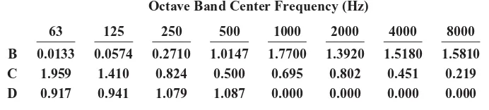
Table14.2 Constants Used in Eq. 14.12 (Reynolds, 1990)
Octave Band Center Frequency (Hz)
63 125 250 500 1000 2000 4000 8000
B 0.0133 0.0574 0.2710 1.0147 1.7700 1.3920 1.5180 1.5810 C 1.959 1.410 0.824 0.500 0.695 0.802 0.451 0.219 D 0.917 0.941 1.079 1.087 0.000 0.000 0.000 0.000
Attenuation in Lined Rectangular Ducts
When a duct is lined with an absorbent material such as a treated fiberglass board, sound prop-agating in the duct is attenuated through its interaction with the material as discussed earlier. A regression equation for the insertion loss of rectangular ducts has been published by Reynolds (1990).
Lduct =B
P S
C
tDl (14.12)
where P=perimeter of the duct (ft) S=area of the duct (sq ft)
l=length of the duct (ft)
t=thickness of the lining (inches) Table 14.2 lists the constants B, C, and D.
Reynolds’ equation was based on data using a 1 to 2 inch (25 mm to 51 mm) thick liner having a density of 1.5 to 3 lbs/ft3 (24 to 48 kg/m3). Linings less than 1 inch (25 mm) thick are generally ineffective. The P/S ratios ranged from 1.1667 to 6, in units of feet. The equation is valid within these ranges.
The insertion loss of ducts is measured by substituting a lined section for an unlined section and reporting the difference. Since there may be a significant contribution to the overall attenuation furnished by the induced motion of the side walls, the unlined attenuation should be added to the lined attenuation to obtain an overall value.
Attenuation of Lined Circular Ducts
An empirical equation for the losses in lined circular ducts has been developed in the form of a third order polynomial regression by Reynolds (1990).
Ld =A+B t+C t2+D d+E d2+F d3 l (14.13)
where t=thickness of the lining (inches) d =interior diameter of the duct (inches)
l=length of the duct (ft) The constants are given in Table 14.3
Table14.3 Constants Used in Eq. 14.13 (Reynolds, 1990)
Freq., Hz A B C D E F
63 0.2825 0.3447 −5.251E-2 −3.837E-2 9.132E-4 −8.294E-6 125 0.5237 0.2234 −4.936E-3 −2.724E-2 3.377E-4 −2.490E-6 250 0.3652 0.7900 −0.1157 −1.834E-2 −1.211E-4 2.681E-6 500 0.1333 1.8450 −0.3735 −1.293E-2 8.624E-5 −4.986E-6 1000 1.9330 0.0000 0.0000 6.135E-2 −3.891E-3 3.934E-5 2000 2.7300 0.0000 0.0000 −7.341E-2 4.428E-4 1.006E-6 4000 2.8000 0.0000 0.0000 −0.1467 3.404E-3 −2.851E-5 8000 1.5450 0.0000 0.0000 −5.452E-2 1.290E-3 −1.318E-5
Because of flanking paths, the duct attenuation in both round and rectangular ducts is limited to 40 dB. As with rectangular ducts, the unlined attenuation may be added to the lined attenuation. For circular ducts it is such a small contribution that it is usually ignored.
Flexible and Fiberglass Ductwork
It is frequently the case that the last duct run in a supply branch is made with a round flexible duct with a lightweight fiberglass fill, surrounded on the outside with a light plastic membrane, and lined on the inside with a fabric liner. The published insertion losses of these flexible ducts are quite high, sometimes as much as 2 to 3 dB per foot or more. Table 14.4 is based on data published in ASHRAE (1995).
Since the insertion loss testing is done by replacing a section of unlined sheet-metal duct with the test specimen, some of the low-frequency loss obtained from flexible duct occurs due to breakout. This property can be used to advantage, since in tight spaces where there is little room for a sound trap, flexible duct surrounded with fiberglass batt can be used to construct a breakout silencer. Such a silencer can be built between joists in a floor-ceiling to isolate exterior noise that might otherwise enter a dwelling through an exhaust duct attached to a bathroom fan. A serpentine arrangement of flexible duct 6 to 8 feet in length in an attic can often control the noise from a fan coil unit located in this space, so long as there is a drywall or plaster ceiling beneath it.
The transmission loss properties of flexible duct are not well documented; however, a conservative approach is to assume that the flex duct is not present and to calculate the insertion loss of the ceiling material. When the attenuation of the flexible duct is greater than the insertion loss of the ceiling the latter is used.
End Effect in Ducts
Table14.4 Lined Flexible Duct Insertion Loss, dB (ASHRAE, 1995)
Diameter Length Octave Band Center Frequency—Hz
(in/mm) (ft/m) 63 125 250 500 1000 2000 4000
4/100 12/3.7 6 11 12 31 37 42 27
9/2.7 5 8 9 23 28 32 20
6/1.8 3 6 6 16 19 21 14
3/0.9 2 3 3 8 9 11 7
5/127 12/3.7 7 12 14 32 38 41 26
9/2.7 5 9 11 24 29 31 20
6/1.8 4 6 7 16 19 21 13
3/0.9 2 3 4 8 10 10 7
6/152 12/3.7 8 12 17 33 38 40 26
9/2.7 6 9 13 25 29 30 20
6/1.8 4 6 9 17 19 20 13
3/0.9 2 3 4 8 10 10 7
7/178 12/3.7 8 12 19 33 37 38 25
9/2.7 6 9 14 25 28 29 19
6/1.8 4 6 10 17 19 19 13
3/0.9 2 3 5 8 9 10 6
8/203 12/3.7 8 11 21 33 37 36 22
9/2.7 6 8 16 25 28 28 18
6/1.8 4 6 11 17 19 19 12
3/0.9 2 3 5 8 9 9 6
9/229 12/3.7 8 11 22 33 37 36 22
9/2.7 6 8 17 25 28 27 17
6/1.8 4 6 11 17 19 18 11
3/0.9 2 3 6 8 9 9 6
10/254 12/3.7 8 10 22 32 36 34 21
9/2.7 6 8 17 24 27 26 16
6/1.8 4 5 11 16 18 17 11
3/0.9 2 3 6 8 9 9 5
12/305 12/3.7 7 9 20 30 34 31 18
9/2.7 5 7 15 23 26 23 14
6/1.8 3 5 10 15 17 16 9
3/0.9 2 2 5 8 9 8 5
14/356 12/3.7 5 7 16 27 31 27 14
9/2.7 4 5 12 20 23 20 11
6/1.8 3 4 8 14 16 14 7
3/0.9 1 2 4 7 8 7 4
16/406 12/3.7 2 4 9 23 28 23 9
9/2.7 2 3 7 17 21 17 7
6/1.8 1 2 5 12 14 12 5
in a baffle and forms a beam. Therefore it does not interact with the sides of the duct and is relatively unaffected by the end effect. An empirical formula for calculating end effect has been published by Reynolds (1990). Its magnitude depends on the size of the duct, mea-sured in wavelengths. This is expressed in the formula as a frequency-width product. The attenuation associated with a duct terminated in free space is
Lend =10 log
and for a duct terminated flush with a wall
Lend =10 log
where d is the diameter of the duct in units consistent with those of the sound velocity. If the duct is rectangular the effective diameter is
d=
4 S
π (14.16)
where S is the area of the duct. End effect attenuation does not occur when the duct is terminated in a diffuser, since these devices smooth the impedance transition between the duct and the room.
Split Losses
When there is a division of the duct into several smaller ducts there is a distribution of the sound energy among the various available paths. The loss is derived in much the same way as was Eq. 8.32; however, multiple areas are taken into account. The split loss in propagating from a main duct into the ithbranch is
Lsplit =10 log
Si =total area of the individual branches that continue on from the main duct(ft2 or m2)
The first term in Eq. 14.17 comes from reflection, which occurs from the change in area, when the total area of the branches is not the same as the area of the main duct and the frequency is below cutoff. The second term comes from the division of acoustic power among the individual branches, which is based on the ratio of their areas.
Elbows
Table14.5 Insertion Loss of Unlined and Lined Square Elbows without Turning Vanes
Insertion Loss, dB
f w Unlined Lined
f w<1.9 0 0
1.9<f w<3.8 1 1 3.8<f w<7.5 5 6 7.5<f w<15 8 11
15<f w<30 4 10
f w>30 3 10
The term f w = f times w, where f is the octave-band center frequency (kHz) and w is the width of the elbow (in).
Table14.6 Insertion Loss of Unlined and Lined Square Elbows with Turning Vanes
Insertion Loss, dB
f w Unlined Lined
f w<1.9 0 0
1.9<f w<3.8 1 1 3.8<f w<7.5 4 4 7.5<f w<15 6 7
f w>15 4 7
The losses in unlined elbows are minimal, particularly if the duct is circular.
Table14.7 Insertion Loss of Round Elbows
f w Insertion Loss, dB
f w<1.9 0 1.9<f w<3.8 1 3.8<f w<7.5 2
f w>15 3
To be considered a lined elbow, the lining must extend two duct widths (in the plane of the turn) beyond the outside of the turn, and the total thickness of both sides must be at least 10% of the duct width. Reynolds (1990) has published data on unlined rectangular elbows, given in Tables 14.5 and 14.6 and for round elbows, shown in Table 14.7.
Figure14.6 Schematic of a Plenum Chamber
from 6 inches to 60 inches (150–1500 mm) in diameter. For elbows where 6 ≤ d ≤ 18 inches (150–750 mm),
Le
d r
2
=0.485+2.094 log(fd)+3.172 [log(fd)]2
−1.578 [log(fd)]4+0.085 [log(fd)]7
(14.18)
and for elbows where 18<d≤60 inches (750–1500 mm),
Le
d r
2
= −1.493+0.538 t+1.406 log(fd)+2.779 [log(fd)]2
−0.662 [log(fd)]4+0.016 [log(fd)]7
(14.19)
where Le=attenuation due to the elbow (dB) d=diameter of the duct (in)
r=radius of the elbow at its centerline (in) t=thickness of the liner (in)
f =center frequency of the octave band (kHz)
Note that if calculated values are negative, the loss is set to zero. In the ducts tested, the elbow radius geometry followed the relationship r=1.5 d+3 t.
14.2 SOUND PROPAGATION THROUGH PLENUMS
A plenum is an enclosed space that has a well-defined entrance and exit, which is part of the air path, and that includes an increase and then a decrease in cross-sectional area. The geometry is shown in Fig. 14.6. A return-air plenum located above a ceiling may or may not be an acoustical plenum. If it is bounded by a drywall or plaster ceiling, it can be modeled as an acoustic plenum; however, if the ceiling is constructed of acoustical tile, it is usually not. Rooms that form part of the air passageway are modeled as plenums. For example a mechanical equipment room can be a plenum when the return air circulates through it. In this case the intake air opening on the fan is the plenum entrance.
Plenum Attenuation—Low-Frequency Case
used in Chapt. 8 for plane waves incident on an expansion and contraction, which was treated in Eqs. 8.35 and 8.36. The transmissivity can be written in terms of the area ratiom=S2/S1
αt = 4
When the plenum is a lined chamber having a certain duct loss per unit length, the wave number k within that space becomes a complex propagation constantq, having an imaginary term jβ. The plenum attenuation is then given by (Davis et al., 1954)
Lp =10 log
The loss term,βl, due to the plenum liner, can be calculated using empirical equations for a lined rectangular duct (Reynolds, 1990)
63 Hz βl=0.00153 (P/S)1.959 t0.917 l
where β =attenuation in the open area of the plenum (nepers/ft or dB/8.68 ft)
P/S=perimeter of the cross - section of the plenum divided by the area (ft−1)
t=thickness of the fiberglass liner (in)
l=length of the plenum (ft)
Plenum Attenuation—High Frequency Case
When the wavelength is not large compared with the dimensions of the central cross section, the plane wave model is no longer appropriate, since the plenum behaves more like a room than a duct. Under these conditions we return to the methodology previously developed for the behavior of sound in rooms. First, we assume that the sound propagating down a duct and into a plenum is nearly plane, so the energy entering the plenum is
and using Eq. 2.74, the direct field intensity at the outlet is
The direct field energy leaving the plenum is
Wo =SocosθIo (14.25)
and the ratio of the direct field outlet energy to the inlet energy is
Wo
A similar treatment can be done for the reverberant energy, with the intensity in a reverberant field, from Eqs. 8.79 and 8.83
Io = Wi
R (14.27)
so that the reverberant field power out is
Wo =SoIo = WiSo
R (14.28)
Combining the direct and reverberant field contributions the overall transmission loss is
Lp =10 logWo
where Lp =attenuation due to the plenum (dB) Si =sound inlet area of the plenum(m2 or ft2)
Qi =directivity of the inlet
So =sound outlet area of the plenum(m2or ft2)
R=room constant of the plenum
=Spα/(1−α) (m2or ft2)
Sp =interior surface area of the plenum(m2or ft2) θ =angle between the inlet and the outlet
When the characteristic entrance dimension is small compared with the inlet to outlet
which assumes that the inlet directivity is one.
These plenum equations begin with the assumption that the inlet and outlet wave-forms are planar. At high frequencies the field at the exit can be semidiffuse rather than planar, particularly above the cutoff frequency. This is similar to the situation encountered in the transmission from a reverberant space through an open door, which was discussed in Chapt. 10. When the inlet condition is semidiffuse and the outlet condition is planar, the plenum is 3 dB more effective than Eq. 14.28 predicts, since there is added attenuation through the conversion of the waveform. If the outlet condition is semidiffuse and the inlet planar, the plenum is 3 dB less effective since there is more energy leaving than predicted by the plane wave relationship. Usually semidiffuse conditions occur when the inlet and outlet openings are large, so that the frequencies are above cutoff, and the upstream and downstream duct lengths are short. If both inlet and outlet conditions are semidiffuse, these relations still hold since the extra energy is passed along from the inlet to the outlet.
Sometimes, the Sabine absorption coefficients of plenum materials are greater than one at certain frequencies, and in many instances a large fraction of the plenum surface is treated with such a material. In these cases the average absorption coefficient may calculate out greater than one, and the room constant is not defined. As a practical guide, when the Norris Eyring room constant is employed a limiting value of the average absorption coefficient should be established, on the order of 0.98.
As was discussed previously, a mechanical plenum is not always an acoustic plenum. For example, if air is returned through the space above an acoustical tile ceiling, the return-air plenum is not an acoustic plenum since the noise breaks out of the space through the acous-tical tile ceiling, which has a transmission loss lower than the theoreacous-tical plenum loss. The problem is treated as if the return-air duct entering the plenum were the source, and the insertion loss of the acoustical tile is subtracted from the sound power level along with the room correction factor to obtain the sound pressure level in the space. Figure 13.15 gives the insertion loss of acoustical tile materials (Blazier, 1981).
In other cases a duct may act as a plenum. If a flexible duct is enclosed in an attic filled with batt insulation, the sound breaks out of the duct and enters the attic plenum space. At the opposite end of the duct it breaks in again, completing the plenum path. This effect can provide significant low-frequency loss in a relatively short distance, particularly when the length of the duct is maximized by snaking. In this manner flexible ducts can be made into quasi-silencers by locating them in joist or attic spaces that are filled with batt.
14.3 SILENCERS
Figure14.7 Duct Silencer Construction
metal filled with fiberglass, which alternate with open-air passage ways. An example is shown in Fig. 14.7.
Dynamic Insertion Loss
Silencer manufacturers publish dynamic insertion loss (DIL) data on their products. This is the attenuation achieved when a given length of unlined duct is replaced with a silencer. Insertion loss data are measured in both the upstream and downstream directions at various air velocities. As with lined ducts, silencer losses in the upstream direction are greater at low frequencies and less at high frequencies.
Insertion loss values are measured in third-octave bands and published as octave-band data. At very low frequencies, below 63 Hz, there are significant comb filtering effects, probably due to the silencer acting as a tuned pipe. In these regions it is more accurate to perform calculations in third-octave bands rather than in octaves. Figure 14.8 gives an example of measured data.
Self Noise
The flow of air through a silencer can generate self noise, and sound power level data are published by silencer manufcturers. Self-noise levels are measured on a 24” × 24” (600×600 mm) inlet area silencer, and a factor of 10 log(S/So)must be added to account
Table14.8 Silencer Self Noise Octave Band Corrections (dB)
Freq. (Hz) 63 125 250 500 1k 2k 4k 8k
Correction 4 4 6 8 13 18 23 28
for the actual area of the silencer being used. In most cases So = 4 ft2 (0.37 sq m), but when the measurements were made on a different unit, the actual face area must be utilized. Self noise is the power radiated from the receiver end of the silencer and is combined with the sound power levels from other sources exiting the silencer. Most of the high-frequency self noise is generated at the air inlet, so it is attenuated in its passage through the silencer in the downstream direction but not in the upstream direction. Hence high-frequency (>1k Hz) self noise levels are greater on the return-air side of an HVAC system. Low-frequency self-noise levels do not vary significantly with flow direction.
When self-noise data are not available, they can be estimated using (Fry, 1988)
Lw ∼=55 log V
V0 +10 log N+10 log H
H0 −45 (14.31)
where Lw =sound power level generated by the silencer (dB) V=velocity in the splitter airway (m / s or ft / min) V0 =reference velocity (1 for m / s and 196.8 for ft / min)
N=number of air passages
H=height or circumfrence (round) of the silencer (mm or in) H0 =reference height (1 for mm or 0.0394 for in)
The spectrum of noise generated by the silencer is calculated by subtracting octave band corrections given in Table 14.8 from the overall sound power level.
Back Pressure
Silencers create some additional back pressure or flow resistance due to the constriction they present. Silencers that minimize this pressure loss are available but there is generally a trade off between back pressure and low-frequency attenuation. Sometimes it is necessary to expand the duct to increase the silencer face area and reduce the pressure loss. It is desirable to minimize the silencer back pressure, usually limiting it to less than 10% of the total rated fan pressure. The position of the silencer in the duct, relative to other components, also affects the back pressure. Figure 14.9 shows published data (IAC Corp.) that give the multiplier of the standard back pressure for various silencer positions.
14.4 BREAKOUT
Figure14.9 Duct Silencer Back Pressure Multipliers (Industrial Acoustics Corp., 1989)
Transmission Theory
The breakout transmission loss defines the relationship between the sound power level enter-ing an incremental slice of the duct at position z and that radiatenter-ing out through the walls of that slice. Figure 14.10 illustrates the geometry (following Ver, 1983).
The breakout transmission loss at a given point is
LTLio =10 log
d Wi(z)
d Wio(z)
(14.32)
where the sound power incident on the increment of duct length, dz is
d Wi(z)=Ii(z) P d z=W i(z)
P
Sd z (14.33)
and the radiated power emanating from this slice on the outside of the duct is
d Wio(z)=d Wi(z)10−0.1LTLio = Wi(z) S 10
−0.1LTLio
P d z (14.34)
If the internal sound power decreases with distance along the duct due to radiation through the duct walls and interaction with the interior surface, according to the relationship
Wi(z)=Wi(0)e−(τ+2β)z (14.35)
the sound power radiated by a lengthlof duct is given by
Wio(z)=
where Lwio=sound power radiated out of the duct (dB) Lwi =sound power level entering the duct (dB)
LTLio =sound transmission loss from the inside to the outside of the duct (dB)
P=perimeter of the duct (m or ft)
l=length of the duct (m or ft)
S=cross sectional area of the duct(m2 or ft2) D, the duct loss term, is defined as
D=10 log
Lduct= attenuation per unit length inside the duct (dB)
τ = P S10
The D term in Eq. 14.39 can be ignored in short sections of duct, particularly when the duct is unlined and unwrapped. However, for lined duct it should be included. In internally lined ducts the attenuation term is usually larger than the breakout term. In flex or fiberglass ducts the breakout term may dominate, though transmission loss data for these products is difficult to obtain. The breakout sound power can never exceed the internal sound power.
Once the sound has penetrated the duct walls it radiates into the room at high frequencies as a normal line source. Equation 8.85 can be used to predict the expected sound pressure level in the room. Alternatively if the duct is long and unlined it radiates like a line source at high frequencies and the sound pressure level is given by
Lp =Lwio+10 log
Q 2πrl +
4 R
+K (14.40)
where K is 0.1 for SI units and 10.5 for FP units.
At low frequencies if the duct is oriented perpendicular to two parallel walls it may excite resonant modes in the room, in which case the simple diffuse field condition does not exist (Ver, 1984).
Transmission Loss of Rectangular Ducts
The duct transmission loss for breakout of rectangular ducts is divided into regions by fre-quency that are similar to those discussed in Chapt. 9 for flat panels (ASHRAE, 1987). The transmission loss behavior with frequency is first stiffness controlled, then mass controlled, and finally coincidence controlled. Figure 14.11 shows the general structure of the loss for rectangular ducts.
For all but very small ducts the fundamental wall resonance falls below the frequency range of interest. In this region there is a minimum transmission loss that is dependent on the duct dimensions (a, b in inches andlin feet)
LTLio(min)=10 log
24l
1 a +
1 b
(14.41)
At higher frequencies, in the mass controlled region, there is a crossover frequency, below which the transmission loss is affected by the duct dimensions, and above which it follows
normal mass law. The crossover frequency is given by
fL = 24120√
a b (14.42)
where a is the larger and b the smaller duct dimension in inches. Below this frequency the transmission loss is given by
LTLio =10 log
f m2s
a+b
+17 (14.43)
where f is the frequency, and msis the duct wall surface mass in lbs/sq ft.
Above the crossover frequency where the normal mass law holds, the transmission loss for steel ducts is given (as in Eq. 9.21) by
LTLio =20 logf ms−KTL (14.44)
where KTL =47.3 in SI units and=33.5 in FP units. At very high frequencies side walls exhibit the normal behavior at the coincidence frequency, but for thin sheet metal this lies above 10 kHz and is of little practical interest.
Transmission Loss of Round Ducts
When sound breaks out of round ducts the definitions in Eq. 14.38 are the same as those
used in rectangular ducts. The inside area is S= πd 2
4 and the outside transmitting area is Pl=12πdl, where d is in inches andlis in feet. The behavior of round ducts is less well understood and more complicated than with rectangular ducts; however, if the analysis is confined to octave bands, the transmission loss can be approximated by a curve, shown in Fig. 14.12. The low-frequency transmission loss is theoretically quite high because the hoop strength of the ducts in their fundamental breathing mode is very large. In practice we do not achieve the predicted theoretical maximum, which may be as high as 80 dB, and a practical limit of 50 dB is used. As the frequency increases the transmission loss is dependent on the localized bending of the duct walls.
Reynolds (1990) has given three formulas to approximate the curve segments shown in Fig. 14.12. The transmission loss is given by the larger of the following two formulas:
LTLio =17.6 log(ms)−49.8 log(f)−55.3 log(d)+Co (14.45)
LTLio =17.6 log(ms)−6.6 log(f)−36.9 log(d)+97.4 (14.46)
where LTLio =sound transmission loss from the inside to the outside of the duct (dB) ms =mass/unit area (lb / sq ft)
d=inside diameter of the duct (in)
Co = 230.4 for long - seam ducts or 232.9 for spiral - wound ducts
In the special case where the frequency is 4000 Hz and the duct is greater than or equal to 26 inches in diameter there is a coincidence effect and
LTLio =17.6 log(ms)−36.9 log(f)+90.6 (14.47)
Since the maximum allowable level is 50 dB, if the calculated level exceeds this limit the transmission loss is set to 50.
Transmission Loss of Flat Oval Ducts
The transmission loss of flat oval or obround ducts falls in between the behavior of square and rectangular ducts. The lower limit of the transmission loss is given by
LTLio =10 log
since if it were any less, according to the definition of transmission loss in Eq. 14.38, it would imply amplification. For obround ducts the areas are given by
S=b(a−b)+πb 2
4 (14.49)
and
Pl=12l [2(a−b)+πb] (14.50)
At low to mid frequencies the wall strength is close to a rectangular duct because of bending of the flat sides. Assuming the radiation is entirely through the flat sides the transmission loss is given by (Reynolds, 1990)
LTLio =10 log
where LTLio =sound transmission loss from the inside to the outside of the duct (dB) ms =mass/unit area (lbs / sq ft)
f =octave band center frequency (Hz) P=perimeter (in)=2(a−b)+πb
δ=fraction of the perimeter taken up by the flat sides
δ= 1
1+ πb 2(a−b)
Figure14.13 Duct Break-in Geometry
14.5 BREAK-IN
The phenomenon known as break-in encompasses the transmission of sound energy from the outside of a duct to the inside. The approach is quite similar to that applied to breakout.
Theoretical Approach
The geometry is shown in Fig. 14.13 and the definition of the transmission loss is similar to that given for breakout.
LTLoi =10 log
d Wo(z) d Woi(z)
(14.52)
where d Wo(z) = IoP d z and Io is the intensity of the diffuse sound field incident on the exterior of the duct. The quantity d Woi(z)is the sound power transmitted from the outside to the inside of the duct by the segment of duct dz, located a distance z from the reference end. The power is given by
d Woi(z)=d Wo(z)10−0.1LTLoi =IoP dz 10−0.1LTLoi (14.53)
The sound then travels down the duct toward the reference end and is attenuated as it is carried along. A factor of two is included since the energy is split with half traveling in each direction. Adding the contributions from all the incremental lengths dz from z = 0 to z=l
Woi(z)=
l
!
0 1
2d Woi(z)e−
(τ+2β)zd z (14.54)
which is
Woi(z)= IoPl
2 10
−0.1LTLio
1−e−(τ+2β)l
(τ+2β)l
and simplifying, we obtain the sound power level at the reference end in terms of the break-in transmission loss
Lwoi=Lwo−LTLoi−3+D (14.56)
where Lwoi =sound power breaking into the duct at a given point (dB) Lwo =sound power level incident on the outside of the duct (dB)
LTLoi =sound transmission loss from the outside to the inside of the duct (dB) D=duct loss correction term (dB)
Ver (1983) has developed simple relationships between the breakout and break-in trans-mission loss values based on reciprocity. Above cutoff where higher order modes can propagate,
LTLoi =LTLio−3 for f >fco (14.57)
and below cutoff,
LTLoi =the larger of ⎧ ⎪ ⎨
⎪ ⎩
LTLio−4+10 loga
b +20 log f fco
10 log Pl 2 S
(14.58)
Note that for round and square ducts, the duct dimensions a and b are equal. The lowest cutoff frequency is given in Eq. 8.21, in terms of the larger duct dimension, a
fco= co
2 a (14.59)
The sound power impacting the exterior of the duct will depend on the type of sound field present in the space. Where the reverberant field predominates, the sound power level incident on the exterior is
Lwo =Lp +10 log Pl−14.5 (14.60)
where Lp is the sound pressure level measured in the reverberant field and the dimensions are in feet.
14.6 CONTROL OF DUCT BORNE NOISE Duct Borne Calculations
A typical duct borne noise transmission problem is illustrated in Fig. 14.14. A fan is located in a mechanical enclosure and transmits noise down a supply duct and into an occupied space. On the return side the ceiling space acts as a plenum for return air, which enters through a lined elbow. There could well be more paths to analyze, such as breakout from the side of a supply or return elbow before the silencer; however, for purposes of this example, we limit it to these two.
Figure14.14 Roof-mounted Built-up Air Handler
Using the fan equations, we can calculate the sound power in octave bands as shown in Table 14.9. We then follow along each path, subtracting the attenuation due to each element and then adding back the sound power that each generates. The computer program used to generate these numbers uses a 0 dB self-noise sound power level as the default value or when calculated levels are negative. This has a slight effect on the very low levels but is of no practical consequence.
Table14.9 HVAC System Loss Calculations, dB
No. Description Octave Band Center Frequency, Hz
63 125 250 500 1000 2000 4000 8000
Supply
1 Fan, Centrifugal, FC—5000 cfm, 2” s.p.
90 86 82 79 77 75 71 61
2 Elbow—36”×24”, Unlined
0 −1 −2 −3 −3 −3 −3 −3
Sum 90 85 80 76 74 72 68 58
Self Noise—0.05” pd
41 39 36 29 20 6 0 0
Combined 90 85 80 76 74 72 68 58
3 Silencer, Standard Pressure Drop Type—3’ long, 36”×24”
−7 −12 −16 −28 −35 −35 −28 −17
Sum 83 73 64 49 39 37 40 41
Self Noise—0.25” pd
49 43 44 42 42 45 35 24
Combined 83 73 64 49 44 45 41 41
Table14.9 HVAC System Loss Calculations, dB (Continued)
No. Description Octave Band Center Frequency, Hz
63 125 250 500 1000 2000 4000 8000
4 Duct, Rectangular Sheet Metal—36”×24”, 5’ long, 1” lining
−2 −2 −3 −7 −15 −12 −11 −9
Sum 81 71 61 42 29 33 30 32
Self Noise
0 0 0 0 0 0 0 0
Combined 81 71 61 42 29 33 30 32
5 Split, 25%
−6 −6 −6 −6 −6 −6 −6 −6
Sum 75 65 55 36 23 27 24 26
Self Noise
0 0 0 0 0 0 0 0
Combined 75 65 55 36 23 27 24 26
6 Duct, Rectangular Sheet Metal—18”×12”, 6’ long, 1” lining
−3 −3 −5 −11 −25 −22 −16 −13
Sum 72 62 50 25 −2 5 8 13
Self Noise
0 0 0 0 0 0 0 0
Combined 72 62 50 25 2 6 9 13
7 Duct, Round Flex Duct—12” diameter, 6’ long
−14 −14 −16 −15 −17 −22 −16 −13
Sum 58 48 34 10 −15 −16 −7 0
Self Noise
0 0 0 0 0 0 0 0
Combined 58 48 34 10 0 0 1 3
8 Rectangular Diffuser, 312 cfm—0.05” pd, 6’ to receiver
0 0 0 0 0 0 0 0
Sum 58 48 34 10 0 0 1 3
Self Noise
33 32 29 23 15 4 0 0
Combined 58 48 35 23 15 5 4 5
Table14.9 HVAC System Loss Calculations, dB (Continued)
No. Description Octave Band Center Frequency, Hz
63 125 250 500 1000 2000 4000 8000
9 Room Effect—20’×20’×8’ Room, Drywall Walls, Carpeted Floor
−6 −6 −5 −5 −6 −7 −6 −6
Sum 52 42 30 18 9 −2 −2 −1
Return
1 Fan, Centrifugal, FC—5000 cfm, 2” s.p.
90 86 82 79 77 75 71 61
2 Elbow—36”×24”, Unlined
0 −1 −2 −3 −3 −3 −3 −3
Sum 90 85 80 76 74 72 68 58
Self Noise 0.05” pd - 4500 cfm
43 42 39 33 24 12 0 0
Combined 90 85 80 76 74 72 68 58
3 Silencer, Low-frequency Standard Pressure Drop Type—5’ long, 36”×24”
−16 −21 −35 −41 −41 −28 −21 −15
Sum 74 64 45 35 33 44 47 43
Self Noise 0.3” pd - 4500 cfm
51 49 53 56 56 59 60 53
Combined 74 64 54 56 56 59 60 53
4 Elbow—36”×24”, Lined, 1”
−1 −2 −3 −4 −5 −6 −8 −10
Sum 73 62 51 52 51 53 52 43
Self Noise 0.05” pd - 4500 cfm
39 38 34 28 18 4 0 0
Combined 73 62 51 52 51 53 52 43
5 Plenum, 2” Duct Liner on Gypboard—800 sq ft, 50% Lined, 8 ft @ 85◦
−12 −13 −19 −20 −20 −20 −21 −21
Sum 61 49 32 32 31 33 31 22
Self Noise
0 0 0 0 0 0 0 0
Combined 61 49 32 32 31 33 31 22
Table14.9 HVAC System Loss Calculations, dB (Continued)
No. Description Octave Band Center Frequency, Hz
63 125 250 500 1000 2000 4000 8000
6 Rectangular Grille—24”×24”, 563 cfm, 0.05” pd, 6’ to receiver
0 0 0 0 0 0 0 0
Sum 61 49 32 32 31 33 31 22
Self Noise
30 29 26 20 12 1 0 0
Combined 61 49 33 33 31 33 31 22
7 Room Effect—20’×20’×8’ Room, Drywall Walls, Carpeted Floor
−9 −8 −6 −8 −8 −8 −9 −10
Sum 52 41 27 25 23 25 22 12
Combined Supply and Return
Supply 52 42 30 18 9 −2 −2 −1
Return 52 41 27 25 23 25 22 12
Combined 55 45 32 26 23 25 22 12
NC 30 57 48 41 35 31 29 28 27
By making the comparison to the room criterion we surmise that the design is satis-factory. We have not checked the breakout level in the plenum through the walls of the first elbow, which should be done. Breakout levels through the walls of a silencer are on the same order as the low-frequency levels passing through the silencer and are not a concern at high frequencies.