Full Terms & Conditions of access and use can be found at
http://www.tandfonline.com/action/journalInformation?journalCode=ubes20
Download by: [Universitas Maritim Raja Ali Haji] Date: 12 January 2016, At: 00:33
Journal of Business & Economic Statistics
ISSN: 0735-0015 (Print) 1537-2707 (Online) Journal homepage: http://www.tandfonline.com/loi/ubes20
Estimating Static Models of Strategic Interactions
Patrick Bajari, Han Hong, John Krainer & Denis Nekipelov
To cite this article: Patrick Bajari, Han Hong, John Krainer & Denis Nekipelov (2010) Estimating
Static Models of Strategic Interactions, Journal of Business & Economic Statistics, 28:4, 469-482, DOI: 10.1198/jbes.2009.07264
To link to this article: http://dx.doi.org/10.1198/jbes.2009.07264
Published online: 01 Jan 2012.
Submit your article to this journal
Article views: 780
Estimating Static Models of Strategic
Interactions
Patrick BAJARI
University of Minnesota and NBER, Minneapolis, MN 55455
Han HONG
Stanford University, Stanford, CA 94305
John KRAINER
Federal Reserve Bank of San Francisco, San Francisco, CA 94105
Denis NEKIPELOV
University of California at Berkeley, Berkeley, CA 94720
We study the estimation of static games of incomplete information with multiple equilibria. A static game is a generalization of a discrete choice model, such as a multinomial logit or probit, which allows the actions of a group of agents to be interdependent. While the estimator we study is quite flexible, in most cases it can be easily implemented using standard statistical packages such as STATA. We also propose an algorithm for simulating the model which finds all equilibria to the game. As an application of our esti-mator, we study recommendations for high technology stocks between 1998–2003. We find that strategic motives, typically ignored in the empirical literature, appear to be an important consideration in the rec-ommendations submitted by equity analysts.
KEY WORDS: Discrete choice; Stock analyst recommendation; Structural estimation.
1. INTRODUCTION
Game theory is one of the most commonly applied tools in economic theory, with substantive applications in all major fields in economics. In some fields, particularly industrial or-ganization, game theory has not only transformed the analysis of market interactions, but also serves as an important basis for policy recommendations. Given the importance of gaming in economic theory, it is not surprising that the empirical analysis of games has been the focus of a recent literature in economet-rics and industrial organization.
In much of the literature, a discrete game is modeled much like a standard discrete choice problem, such as the multino-mial logit. An agent’s utility is often assumed to be a linear function of covariates and a random preference shock. How-ever, unlike a discrete choice model, utility is also allowed to depend on the actions of other agents. A discrete game strictly generalizes a standard random utility model, but does not impose the often strong assumption that agents act in isola-tion. Early attempts at the econometric analysis of such games included Bjorn and Vuong (1984) and Bresnahan and Reiss (1991a, 1991b). Recent contributions includeHaile, Hortacsu, and Kosenok(2008),Aradillas-Lopez(2008),Ho(2009),Ishii (2008),Pakes et al.(2007),Augereau, Greenstein, and Rysman (2006),Seim(2006),Sweeting(2008), andTamer (2003). In particular,Aguirregabiria and Mira(2002) propose a two-step method to estimate static games of incomplete information and illustrate it using an example of a static game of market entry.
An important insight in the recent literature is that it is often most straightforward to estimate discrete games in two steps. The static model of strategic interaction with incomplete infor-mation is a particular case when the discount rate is zero of the
dynamic games considered inAguirregabiria and Mira(2007), Bajari, Benkard, and Levin(2007),Berry, Pakes, and Ostrovsky (2007), andPesendorfer and Schmidt-Dengler(2003). In a first step, the economist estimates the reduced forms implied by the model. This often boils down to using standard econometric methods to estimate the probability that one of the finite num-ber of possible choices is observed, conditional on the relevant covariates. In the second step, the economist estimates a single agent random utility model, including as controls the equilib-rium beliefs about the behavior of others from the first step.
In this paper, we study semiparametric estimation of static games of strategic interaction with multiple equilibria. Like the two-step approach discussed above, we estimate the reduced form choice probabilities in a first stage, and use them to sim-plify the estimation of the finite dimensional mean payoff para-meters in the second stage.
The two-step approach pioneered inAguirregabiria and Mira (2007) can be implemented both nonparametrically and semi-parametrically. It is closely related to nonparametric identifica-tion of the mean utility funcidentifica-tions, does not depend on whether the first-stage regressors are discrete or continuous, and does not require a correctly specified first-stage parametric model. The two-step estimator has desirable computational and statis-tical properties. First, when the regressors are continuous, de-spite the fact the first stage is nonparametric and might con-verge at a slow rate, the structural parameters estimated in the second stage have normal asymptotics and converge at a rate
© 2010American Statistical Association Journal of Business & Economic Statistics October 2010, Vol. 28, No. 4 DOI:10.1198/jbes.2009.07264
469
proportional to the square root of the sample size. This fol-lows from arguments based onNewey(1994). Under suitable regularity conditions, the asymptotic variance of the second stage estimator is invariant to whether the first stage nonpara-metric estimator is implemented using kernel methods or sieve methods. Second, in many cases the two-step nonparametric and semiparametric estimators can be implemented with cor-rect standard errors using a two-stage least squares procedure in a standard statistical package like STATA. The simplicity of this approach makes the estimation of these models accessible to a larger audience of researchers.
In the context of discrete regressors, Pesendorfer and Schmidt-Dengler (2003) demonstrate that exclusion restrictions are sufficient for identification in a particular set of dynamic entry games. A related exclusion restriction, which excludes payoff-relevant covariates for a particular player from the util-ities of the other players, is also required when the regressors are continuous. For instance, in an entry model, if the produc-tivity shock of firmiinfluences its own entry decision, but only indirectly influences the entry decisions of other firms, then the mean payoff function is nonparametrically identified. The condition for nonparametric identification can be formulated as standard rank conditions for an appropriately defined lin-ear system regardless of whether the regressors are continuous or discrete. This identification strategy relies crucially on the assumption that data in each market is generated from a sin-gle equilibrium. An alternative identification strategy that is not considered in this paper is to search for events that change which equilibrium to the game is played, but otherwise do not influence payoffs.Sweeting(2008) demonstrates that multiplic-ity of equilibrium can assist with identification in a symmetric location game.
The assumption that the data come from a single equilib-rium has very different implications for discrete and continuous explanatory variables. If the vector of observable explanatory variables has a discrete support and the nonparametric estima-tor in the first step does not impose any smoothness condition (e.g., an unrestricted frequency estimator), then the assump-tion needed is that for a given value of explanatory variables, the data come from the same equilibrium. However, when the explanatory variables contain continuous variables, the first-step estimator usually imposes smoothness conditions for the second-step estimator to converge at a parametric rate to a nor-mal distribution. This requires smoothness conditions with re-spect to continuous state variables in the equilibrium selec-tion mechanism. These smoothness condiselec-tions can be stated in terms of pseudo-norms and may not allow for nondifferentiabil-ity in a set of measure zero; see, for example,Chen, Linton, and Van Keilegom(2003). In the presence of multiple equilibria, the points of nondifferentiability typically occurs when the equilib-rium path bifurcates. The smoothness condition does require the equilibrium paths to not bifurcate for almost all values of the continuous state variable, or a smooth path is chosen at the points of bifurcation. If a substantial amount of discontinuity is present in selecting among multiple equilibria of the game, in which case an alternative approach is to incorporate an equi-librium selection mechanism using exclusion restrictions, ei-ther a full solution method or a version of the recursive method proposed byAguirregabiria and Mira(2007) applied to a static game must be used.
As an application of our methods, we model the determina-tion of stock recommendadetermina-tions (e.g., strong buy, buy, hold, sell) issued by equity analysts for high technology stocks listed in the NASDAQ 100 between 1998 and 2003. The determination of recommendations during this time period is of particular in-terest in the wake of the sharp stock price declines for technol-ogy firms in 2000. Recommended stocks underperformed the market as a whole during this period by a wide margin. Highly publicized allegations of conflicts of interest have called into question whether analysts were more concerned with helping their firms win investment banking business than with produc-ing accurate assessments of the prospects of the firms under scrutiny. While there is a fairly large literature in finance on recommendations, we are not aware of any papers that formally consider the simultaneity of recommendations due to strategic motives.
In our model, recommendations submitted by analysts de-pend on four factors. First, recommendations must dede-pend on fundamentals and commonly shared expectations about the fu-ture profitability of the firm. These expectations will be embed-ded in the stock price. Second, analysts are heterogeneous, both in terms of talent and perhaps in terms of access to information. We try to capture an individual analyst’s private belief about the stock by looking at the difference between the quarterly earnings forecast submitted by the analyst (or the analyst’s bro-kerage firm) and the distribution of forecasts from other firms. Mindful of the large number of inquiries into possible conflicts of interest among research analysts, we include as a third fac-tor a dummy variable for an investment banking relationship between the firm and the analyst’s employer.
Finally, we consider the influence of peers on the recommen-dation decision. Peer effects can impact the recommenrecommen-dation in different ways. Individual analysts have incentive to condition their recommendation on the recommendations of their peers, because even if their recommendations turn out to be unprof-itable ex-post, performance evaluation is typically a compari-son against the performance of peers. More subtly, recommen-dations are relative rankings of firms and are not easily quan-tifiable (or verifiable) objects. As such, ratings scales usually reflect conventions and norms. The phenomenon is similar to the college professor’s problem of assigning grades. If a pro-fessor were to award the average student with a C while other faculty gave a B+to the average student, the professor might incorrectly signal his views of student performance. Even while there is heterogeneity in how individual professors feel about grading, most conform to norms if only to communicate clearly with students (and their potential employers) about their per-formance. Similarly, analysts might have an incentive to bench-mark their recommendations against perceived industry norms. The paper is organized as follows. In Section2 we outline the general economic environment. For purposes of exposition, we develop many of the key formulae within the context of a simple entry model. In Section3 we discuss the problem of nonparametric identification of the mean payoff functions. In Section4we show how to derive nonparametric and semipara-metric estimates of the structural parameters for our class of models. Section5contains the empirical application to equity analyst recommendations. Section6concludes the paper.
2. THE MODEL
In the model, there are a finite number of players, i =
1, . . . ,nand each player simultaneously chooses an actionai∈
{0,1, . . . ,K}out of a finite set. We restrict players to have the same set of actions for notational simplicity. However, all of our results will generalize to the case where all players have differ-ent finite sets of actions. LetA= {0,1, . . . ,K}ndenote the vec-tor of possible actions for all players and leta=(a1, . . . ,an)
denote a generic element of A. As is common in the litera-ture, we leta−i=(a1, . . . ,ai−1,ai+1, . . . ,an)denote a vector
of strategies for all players, excluding playeri. We will abstract from mixed strategies since in our model, with probability one each player will have a unique best response.
Letsi∈Sidenote the state variable for playeri. LetS=iSi
and lets=(s1, . . . ,sn)∈Sdenote a vector of state variables for
allnplayers. We will assume thatsis common knowledge to all players in the game and in our econometric analysis, we will as-sume thatsis observable to the econometrician. The state vari-able is assumed to be a real valued vector, butSiis not required
to be a finite set. Much of the previous literature assumes that the state variables in a discrete game lie in a discrete set. While this assumption simplifies the econometric analysis of the esti-mator and identification, it is a strong assumption that may not be satisfied in many applications.
For each agent, there are alsoK+1 state variables which we label asǫi(ai)which are private information to each agent.
These state variables are distributed iid across agents and ac-tions. Let ǫi denote the 1×(K+1)vector of the individual
ǫi(ai).The density ofǫi(ai)will be denoted asf(ǫi(ai)).
How-ever, we shall sometimes simplify the notation and denote the density forεi=(εi(0), . . . , εi(K))asf(ǫi).
The period utility function for playeriis
ui(a,s, ǫi;θ )=πi(ai,a−i,s;θ )+ǫi(ai). (1)
The utility function in our model is similar to a standard ran-dom utility model such as a multinomial logit. Each playeri
receives a stochastic preference shock,ǫi(ai),for each
possi-ble action ai. In many applications, this will be drawn from
an extreme value distribution as in the logit model. In the literature, the preference shock is alternatively interpreted as an unobserved state variable (see Rust1994). Utility also de-pends on the vector of state variablessand actionsa through
i(ai,a−i,s;θ ). For example, in the literature, this part of
util-ity is frequently parameterized as a simple linear function of ac-tions and states. Unlike a standard discrete choice model, how-ever, note that the actionsa−iof other players in the game enter
intoi’s utility. A standard discrete choice model typically as-sumes that agentsiact in isolation in the sense thata−iis
omit-ted from the utility function. In many applications, this is an implausible assumption.
In this model, player i’s decision rule is a function ai =
δi(s, ǫi). Note thati’s decision does not depend on theǫ−isince
these shocks are private information to the other−iplayers in the game and, hence, are unobservable toi. Defineσi(ai|s)as
σi(ai=k|s)=
1{δi(s, ǫi)=k}f(ǫi)dǫi.
In the above expression, 1{δi(s, ǫi)=k}is the indicator
func-tion that playeri’s action is k given the vector of state vari-ables (s, ǫi). Therefore, σi(ai =k|s) is the probability that i
chooses action kconditional on the state variables sthat are public information. We will define the distribution ofagivens
asσ (a|s)=n
ing ai when the vector of parameters is θ. Since i does not
know the private information shocks, ǫj for the other
play-ers,i’s beliefs about their actions are given byσ−i(a−i|s).The
term
a−ii(ai,a−i,s, θ )σ−i(a−i|s)is the expected value of
i(ai,a−i,s;θ ), marginalizing out the strategies of the other
players usingσ−i(a−i|s). The structure of payoffs in (2) is quite
similar to standard random utility models, except that the prob-ability distribution over other agents’ actions enter into the for-mula for agenti’s utility. Note that if the error term has an atom-less distribution, then playeri’s optimal action is unique with probability one. This is an extremely convenient property and eliminates the need to consider mixed strategies as in a standard normal form game.
We also define the deterministic part of the expected payoff as
i(ai,s;θ )=
a−i
πi(ai,a−i,s, θ )σ−i(a−i|s). (3)
It follows immediately then that the optimal action for playeri
satisfies
σi(ai|s)=Prob{ǫi|i(ai,s;θ )+ǫi(ai)
> i(aj,s;θ )+ǫi(aj)forj=i}. (4) 2.1 A Simple Example
For expositional clarity, consider a simple example of a dis-crete game. Perhaps the most commonly studied example of a discrete game in the literature is a static entry game (see Bresna-han and Reiss1991a, 1991b;Berry 1992;Tamer 2003;Ciliberto and Tamer 2009, andManuszak and Cohen 2004). In the em-pirical analysis of entry games, the economist typically has data on a cross section of markets and observes whether a particular firmichooses to enter a particular market. InBerry(1992) and Ciliberto and Tamer(2009), for example, the firms are major United States airlines such as American, United, and Northwest and the markets are large, metropolitan airports. The state vari-ables,si, might include the population in the metropolitan area
surrounding the airport and measures of an airline’s operating costs. Letai=1 denote the decision to enter a particular market
andai=0 denote the decision not to enter the market. In many
applications,πi(ai,a−i,s;θ )is assumed to be a linear function,
In Equation (5), the mean utility from not entering is set equal to zero. We formally discuss this normalization in our section on identification. The termδ measures the influence ofj’s choice on i’s entry decision. If profits decrease from having another firm enter the market thenδ <0.The parametersβmeasure the impact of the state variables onπi(ai,a−i,s).
The random error termsεi(ai)are thought to capture shocks
to the profitability of entry that are private information to firmi. Suppose that the error terms are distributed extreme value. Then, utility maximization by firmiimplies that fori=1, . . . ,n
σi(ai=1|s)=
exps′·β+δ
j=iσj(aj=1|s)
1+exp
s′·β+δ
j=iσj(aj=1|s)
(6)
=Ŵi(β, δ, σj(1|s),∀j).
In the system of equations above, applying the formula in Equa-tion (3) implies thati(ai,s;θ )=s′·β+δj=iσj(aj=1|s).
Since the error terms are distributed extreme value, Equation (4) implies that the choice probabilities σi(ai=1|s)take a form
similar to a single agent multinomial logit model. We note in passing that it can easily be shown using Brouwer’s fixed point theorem that an equilibrium to this model exists for any finites
(seeMcKelvey and Palfrey 1995).
We exploit the convenient representation of equilibrium in Equation (6) in our econometric analysis. Suppose that the econometrician observest=1, . . . ,T repetitions of the game. Letai,tdenote the entry decision of firmiin repetitiontand let
the value of the state variables be equal tost. By observing
en-try behavior in a large number of markets, the econometrician could form a consistent estimateσˆi(ai=1|s)ofσi(ai=1|s)for
i=1, . . . ,n. In an application, this simply boils down to flexi-bly estimating the probability that a binary response,ai, is equal
to one, conditional on a given set of covariates. This could be done using any one of a number of standard techniques. Given first-stage estimates ofσˆi(ai=1|s), we could then estimate the
structural parameters of the payoff, β and δ, by maximizing a pseudo-likelihood function using Ŵi(β, δ,σˆj(1|s),∀j). There
are two attractive features to this strategy. The first is that it is not demanding computationally. First-stage estimates of choice probabilities can be done using a strategy as simple as a lin-ear probability model. The computational burden of the second stage is also light since we only need to estimate a logit model. A second attractive feature is that it allows us to view a game as a generalization of a standard discrete choice model. Thus, techniques from the voluminous econometric literature on dis-crete choice models can be imported into the study of strategic interaction. While the example considered above is simple, it nonetheless illustrates many of the key ideas that will be essen-tial in what follows.
We can also see a key problem with identification in the sim-ple examsim-ple above. Both the first-stage estimatesσˆi(ai=1|s)
and the term s′·β depend on the vector of state variables s. This suggests that we will suffer from a collinearity problem when trying to separately identify the effects ofβ andδ on the observed choices. The standard solution to this type of prob-lem in many settings is to impose an exclusion restriction. Sup-pose, for instance, a firm specific productivity shock is included ins. In most oligopoly models, absent technology spillovers, the productivity shocks of firms−iwill not directly enter into
firmi’s profits. These shocks only enter indirectly through the endogenously determined actions of firms −i, for example, price, quantity, or entry decisions. Therefore, if we exclude the productivity shocks of other firms from the terms′·β, we will no longer suffer from a collinearity problem. While this idea is quite simple, as we shall discover in the next section, similar restrictions are required to identify more general models.
3. IDENTIFICATION
In this section, we consider the problem of identifying the de-terministic part of payoffs, without making particular assump-tions about its functional form (e.g., that it is a linear index as in the previous example). In the context of this section, we letθ
be completely nonparametric and writeπi(ai,a−i,s)instead of
πi(ai,a−i,s;θ ).
Definition 1. We will say that πi(ai,a−i,s) is identified if
πi(ai,a−i,s)=πi′(ai,a−i,s)for somei=1, . . . ,nimplies that
for the corresponding equilibrium choice probabilitiesσi(ai=
1|s)=σi′(ai=1|s)for somei=1, . . . ,n.
Formally, identification requires that different values of the primitives generate different choice probabilities. If this con-dition is not satisfied, then it will be impossible for us to uniquely recover the structural parameters πi(ai,a−i,s) (for
i=1, . . . ,n) from knowledge of the observed choice probabil-ities,σi(ai=1|s). While the mean payoff function is
nonpara-metric, the model is semiparametric because the distribution of the unobservables is parametrically specified. Even in a single agent problem, it is well known that it is not possible to non-parametrically identify both the mean utility functions and the joint distribution of the error termsF(ǫi)without making strong
exclusion and identification at infinity assumptions (see, e.g., Matzkin 1992).
To take the simplest possible example, consider a simple bi-nary response model and assume that the error terms are nor-mally distributed, as in the probit model. Letσi(ai=1|s)
de-note the probability that the response is equal to one in the data conditional ons. Definei(ai=0|s)=0 andi(ai=1|s)=
F−1(σi(ai=1|s)), whereF−1 denotes the normal cdf. It can
easily be verified that this definition ofiperfectly rationalizes
any set of choice probabilitiesσi(ai=1|s). Since even a single
agent discrete choice model is not identified without a paramet-ric assumption on the error term, assumptions at least as strong will be required in the more general setup with strategic interac-tions. In what follows, we will typically impose the assumption that the error terms are distributed iid with a known distrib-ution function, since both independence and parametric form assumption on the error terms are required for identification.
Based on the discussion above, we shall impose the following assumption in order to identify the model:
A1. The error terms ǫi(ai) are distributed iid across
ac-tionsaiand agentsi. Furthermore, the parametric form
of the distributionFcomes from a known family.
Analogous to the notation in the previous section, define
i(k,s)=a−iπi(ai=k,a−i,s)σ−i(a−i|s). It is
straightfor-ward to show that the equilibrium in this model must satisfy
δi(s, ǫi)=k if and only if
(7)
i(k,s)+ǫi(k) > i(k′,s)+ǫi(k′) for allk′=k.
That is, actionkis chosen if and only if the deterministic ex-pected payoff and error term associated with actionkis greater than the analogous values of k′=k. An implication of (7) is that the equilibrium choice probabilitiesσi(a|s)must satisfy
σi(ai|s)=Pr
ǫi(ai)+i(ai,s)−i(0,s)
> ǫi(k)+i(k,s)−i(0,s),
∀k=0, . . . ,K,k=ai. (8)
Equation (8) is a simple consequence of (7) where we can sub-tracti(0,s)from both sides of the inequality.
Suppose we generate ǫi(ai) from an extreme value
distri-bution as in the multinomial logit model. Then (8) implies thatσi(ai|s)=exp(i(ai,s)−i(0,s))/(Kk=0exp(i(k,s)−
i(0,s))).Alternatively, in an ordered logit model, for the
lo-gistic function(·),σi(ai=k|s)=(i(k+1,s))−(i(k,
s)). A key insight similar to Hotz and Miller (1993) is that Equation (8) implies that the equilibrium choice probabilities,
σi(ai|s),have a one-to-one relationship to the “choice specific
value functions,” i(ai,s)−i(0,s). It is obvious that we
should expect the one-to-one mapping in any model where the distribution ofǫi has full support. We letŴ:{0, . . . ,K} ×S→
[0,1] denote the map in general from choice specific value functions to choice probabilities, that is,
(σi(0|s), . . . , σi(K|s))
=Ŵi(i(1,s)−i(0,s), . . . , i(K,s)−i(0,s)). (9)
We will denote the inverse mapping byŴ−1:
(i(1,s)−i(0,s), . . . , i(K,s)−i(0,s))
=Ŵi−1(σi(0|s), . . . , σi(K|s)). (10)
The above analysis implies that we can invert the equilibrium choice probabilities to nonparametrically recover i(1,s)−
i(0,s), . . . , i(K,s)−i(0,s). However, the above analysis
implies that we will not be able to separately identifyi(1,s)
andi(0,s); we can only identify the difference between these
two terms. Therefore, we shall impose the following assump-tion:
A2. For alliand alla−iands,πi(ai=0,a−i,s)=0.
The above assumption is similar to the “outside good” assump-tion in a single-agent model where the mean utility from a par-ticular choice is set equal to zero. In the context of the entry model, this assumption is satisfied if the profit from not enter-ing the market is equal to zero regardless of the actions of other agents. Just as in the single-agent model, there are alternative normalizations that we could use to identify theπi(ai,a−i,s).
However, for expositional simplicity we shall restrict attention to the normalization in A2.
Given assumption A2 and knowledge of the equilibrium choice probabilities,σi(ai|s), we can then apply the mapping
in (10) to recover i(ai,s)for alli,ai, and s. Recall that the
definition ofi(ai,s)implies that
i(ai,s)=
a−i
σ−i(a−i|s)πi(ai,a−i,s),
∀i=1, . . . ,n,ai=1, . . . ,K. (11)
Even if we know the values of i(ai,s)andσ−i(a−i|s)in
the above equation, it is not possible to uniquely determine the values ofπi(ai,a−i,s). To see why, hold the state vectorsfixed,
then determination of the utilities of all agents involves solving forn×K×(K+1)n−1unknowns. That is, there arenagents, for each actionk=1, . . . ,K, utility depends on the(K+1)n−1
possible actions of the other agents. However, the left-hand side of (11) only contains information aboutn×(K+1)scalars holdingsfixed. It is clearly not possible to invert this system in order to identifyπi(ai,a−i,s)for alli, allk=1, . . . ,K, and all
a−i∈A−i.
Obviously, there must be cross-equation restrictions across either i or k in order to identify the system. One way to identify the system is to impose exclusion restrictions. Parti-tions=(si,s−i), and supposeπi(ai,a−i,s)=πi(ai,a−i,si)
de-pends only on the subvectorsi. We can demonstrate this in the
context of an entry model. In this type of model, the state is usu-ally a vector of productivity shocks. While we might expect the profit of firmito depend on the entry decisions of other agents, it should not depend on the productivity shocks of other agents. If such an exclusion restriction is possible, we can then write
i(ai,s−i,si)=
a−i
σ−i(a−i|s−i,si)πi(ai,a−i,si). (12)
Clearly, a necessary order condition for identification is that for eachsi, there exists(K+1)n−1points in the support of the
con-ditional distribution of s−i givensi. Note that this assumption
will be satisfied as long ass−icontains a continuously
distrib-uted variable with i(ai,a−i,si) sufficiently variable. A
suf-ficient rank condition will require that for almost all si, the
system of equations obtained by varying the values of s−i is
nonsingular and invertible.
Theorem 1. Suppose that A1 and A2 hold. A necessary or-der condition for identifying the latent utilities i(ai,a−i,si)
is that for almost all si, there exists (K +1)n−1 points in
the support of the conditional distribution of s−i given si.
A sufficient rank condition for identification is that for al-most all values ofsi, the conditional second moment matrix of
E[σ−i(a−i|s−i,si)σ−i(a−i|s−i,si)′|si]is nonsingular.
Note that the rank condition holds regardless of whether the regressors are discrete or continuous. Because the rank condi-tion is stated in terms of the observable reduced form choice probabilities, it is a testable assumption that can be verified from the data. It is analogous to the standard rank condition in a linear regression model. The difference is that the “regres-sors,”σ−i(a−i|s−i,si)themselves have to be estimated from the
data in the first stage. Intuitively, to identify strategic interaction models in which the primitive payoffs depend on the expected action of the opponent, the reduced form choice probabilities are required to depend on the opponent’s idiosyncratic states. In the single-agent model with no strategic interactions, the left-hand side of (12) does not depend ons−iand the right hand side
does not depend ona−i. The probabilitiesσ−i(a−i|s−i,si)sum
up to one, and Equation (12) becomes an identity.
4. ESTIMATION
In the previous section, we demonstrated that there is a nonparametric inversion between choice probabilities and the choice-specific value functions, (ai,s). Furthermore, we
demonstrated that the structural parameters of our model are identified if appropriate exclusion restrictions are made on pay-offs. In this section, we exploit this inversion to construct non-parametric and seminon-parametric estimates of our structural para-meters.
Step 1: Estimation of Choice Probabilities. Suppose the economist has access to data ont=1, . . . ,T repetitions of the game. For each repetition, the economist observes the actions and state variables for each agent(ai,t,si,t). In the first step we
form an estimateσˆi(k|s)ofσi(k|s)using sieve series expansions
(seeNewey 1990andAi and Chen 2003). We note, however, that we could alternatively estimate the first stage using other nonparametric regression methods such as kernel smoothing or local polynomial regressions.
The usual approach in the nested fixed point algorithm is to discretize the state space, which is only required to be precise enough subject to the constraints imposed by the computing fa-cility. However, increasing the number of grids in a nonpara-metric or two-stage semiparanonpara-metric method has two offsetting effects. It reduces the bias in the first-stage estimation but in-creases the variance. In fact, when the dimension of the contin-uous state variables is larger than four, it can be shown that it is not possible to obtain√T consistency through discretization and asymptotically normal parameter estimates in the second stage, where T is the sample size. Therefore, discretizing the state space does not provide a solution to continuous state vari-ables, which requires a more refined econometric analysis.
Let {ql(s),l =1,2, . . .} denote a sequence of known
ba-sis functions that can approximate a real valued measurable function of s arbitrarily well for a sufficiently large value of l. The sieve could be formed using splines, Fourier Series, or orthogonal polynomials. We let the basis become increas-ingly flexible as the number of repetitions of the game T be-comes large. Let κ(T) denote the number of basis functions to be used when the sample size is T. We shall assume that
κ(T)→ ∞, κ(T)/T →0 at an appropriate rate to be speci-fied below. Denote the 1×κ(T)vector of basis functions as
qκ(T)(s)=(q1(s), . . . ,qκ(T)(s)), and its collection into a
regres-Equation (13) is the standard formula for a linear probability model where the regressors are the sieve functionsqκ(T)(s). We note that in the presence of continuous state variables, the sieve estimatorσˆi(k|s)will converge to the trueσi(k|s)at a
nonpara-metric rate slower than√T.
Second Step: Inversion. In our second step, we take as given our estimatesσˆi(k|s)of the equilibrium choice probabilities. We
then form an estimate of the expected deterministic utility func-tions,ˆi(k,st)− ˆi(0,st)for k=1, . . . ,K andt=1, . . . ,T.
In the specific case of the binary logit model, this inversion would simply be
ˆ
i(1,st)− ˆi(0,st)=log(σˆi(1|st))−log(σˆi(0|st)).
In an alternative model, such as one with normal shocks, we would need to solve a nonlinear system. In what follows, we shall impose A2 so thatˆi(0,s)= ˆi(0,a−i,s)=0 for alla−i.
Third Step: Recovering the Structural Parameters. In the first step we recovered an estimate ofσˆi(ai,s)and in the
sec-ond step we recovered an estimate of the choice specific value functionˆi(k,s). In our third step, we use the empirical analog
of (11) to form an estimate ofπ(ai,a−i,si). We shall assume
that we have made a sufficient number of exclusion restrictions, as discussed in the previous section, so that the model is iden-tified. For a given value ofsi, for a givena=(ai,a−i), we
esti-where the nonparametric weightsw(t,si)can take a variety of
forms. For example,
uses kernel weights, and other local weights are also possible. The identification condition in the previous section ensures that the regressor matrix in this weighted least squares regression is nonsingular asymptotically.
4.1 A Linear Model of Utility
The nonparametric estimation procedure described in the previous section follows the identification arguments closely and offers the advantage of flexibility and robustness against misspecification. However, without a huge amount of data, non-parametric estimation methods can be subject to a severe curse of dimensionality when we intend to control for a large di-mension of state variables s. Also, in small samples, differ-ent implemdiffer-entations of nonparametric procedures may lead to drastically different point estimates. Therefore, in the following we consider a semiparametric estimation where the determinis-tic utility componentsπi(ai,a−i,s)are specified to be a linear
function of a finite dimensional parameter vectorθ. This is the typical econometric specification that is commonly used in the empirical literature. In this section we describe a straightfor-ward estimation and inference procedure for this model.
The mean utility is assumed to take the form ofπi(ai,a−i,
si)=i(ai,a−i,si)′θ. In the above expression, the
determin-istic part of utility is a linear combination of a vector of ba-sis functions,i(ai,a−i,si). For instance, we might let utility
be a linear index as in our simple entry game example of the previous section. Alternatively, we might choosei(ai,a−i,si)
to be a standard flexible functional form, such as a high-order polynomial, spline function, or orthogonal polynomial. The es-timator we discuss below can easily be generalized to allow for the possibility thatθenters the utility nonlinearly. However, the exposition of the properties of the estimator is facilitated by the linearity assumption. Also, most applications of discrete choice models and discrete games usually are linear in the structural parameters of interest.
This linearity assumption implies that the choice specific value function, given ai and s, takes the convenient form
i(ai,s)=E[πi(ai,a−i,si)|s,ai] =i(ai,s)′θ, wherei(ai,s)
If we defineσ (s)to be the stacked vector of choice probabili-tiesσi(k|s)for allk=1, . . . ,K,i=1, . . . ,n, then we can
col-lect (14) into a fixed point mapping: σ (s)=Ŵ(σ (s)). To em-phasize the dependence on the parameterθ, we can also write
σ (s;θ )=Ŵ(s, θ;σ (s;θ )). (15) 4.2 Semiparametric Estimation
Step 1: Estimation of Choice Probabilities. The simple semiparametric procedure we propose proceeds in two steps. We begin by forming a nonparametric estimate of the choice probabilities,σˆi(k|s). We will do this like above using a sieve
approach, though one could alternatively use kernels or a local polynomial method.
Given our estimates of the choice probabilities, we can then estimatei(k,s)correspondingly by
For instance, take the example presented in (5). In this ex-ample,i(ai=1,a−i,s)=(s,j=i1{aj=1})·(β, δ), where
“·” denotes an inner product. Thus, in the above formula,
′i(ai=1,a−i,s)=(s,j=i1{aj=1})andθ=(β, δ). Then,
given our first-stage estimates of the choice probabilities,
ˆ
′(ai =1,a−i,s)=(s,j=i1{aj =1}σj(aj|s)). For each
pa-rameter value θ, we can evaluate the empirical analogue of (15). For example, in the binary logit case, it is denoted as
σi(ai=1|s,, θ )ˆ .
Step 2: Parameter Estimation. In the second stage, a vari-ety of estimators can be used to recover the value ofθ. Most of these estimators can be written as GMM estimators with a properly defined set of instruments. To describe the second stage, define yikt =1 if ait =k and yikt =0 otherwise, for
in the first stage (such as two-step optimally weighted GMM), or may be estimated simultaneously (such as pseudo MLE). It is well known that the estimation errors inAˆ(st)will not affect
the asymptotic distribution ofθˆdefined by (17), regardless of whetherAˆ(st)is estimated in a preliminary step or is estimated
simultaneously withθˆ. Therefore, next we will focus on deriv-ing the large sample properties ofθˆdefined by (17) whereA(st)
is known.
The estimator that we consider falls within the class of semi-parametric estimators considered by Newey(1994). A some-what surprising conclusion is that even though the first stage is estimated nonparametrically and can be expected to converge at a rate slower than√T, the structural parameters will be as-ymptotically normal and will converge at a rate of√T. More-over, under appropriate regularity conditions, the second stage asymptotic variance will be independent of the particular choice of nonparametric method used to estimate the first stage (e.g., sieve or kernel). As a practical matter, these results justify the use of the bootstrap to calculate standard errors for our model.
In theAppendix, we derive the following result, applying the general framework developed byNewey(1990). Under appro-priate regularity conditions, the asymptotic distribution ofθˆ de-fined in (17) satisfies
√
T(θˆ−θ )−→d N(0,G−1G−1′),
whereG=EA(st)∂θ∂ σ (st, 0, θ0), andis the asymptotic
vari-ance ofA(st)(yt−σ (st,, θˆ 0)). In theAppendix, we also
com-pare the asymptotic variance of alternative estimators.
4.3 Market Specific Payoff Models
If a large panel data with a large time dimension for each market is available, both the nonparametric and semiparamet-ric estimators can be implemented market by market to allow for a substantial amount of unobserved heterogeneity. Even in the absence of such rich datasets, market specific payoff effects can still be introduced into the two-step estimation method if we are willing to impose a somewhat strong assumption on the market specific payoffs,αt, which is observed by all the players
in that market but not by the econometrician. We will assume
thatαtis an unknown but smooth function of the state variables
st=(st1, . . . ,stn)in that market, which we will denote asα(st).
In principal, we would prefer a model where the fixed effect was not required to be a function of the observables. However, in highly nonlinear models, such as ours, similar assumptions are commonly made. See, for example,Newey(1994). Strictly speaking, our assumption is stronger than and impliesNewey (1994), who only assumes that sum ofαtand the idiosyncratic
errors is homoscedastic and normal conditional on the observed state variables. This assumption, albeit strong, is convenient technically since it implies that the equilibrium choice proba-bilities,σi, can still be written as a function of the statest.
With the inclusion of a market-specific component, the mean period utility function in (1) for playeriin markettis now mod-ified to πi(ai,a−i,s)=α(ai,s)+ ˜πi(ai,a−i,s). In the above,
and what follows, we drop the market specific subscript tfor notational simplicity.
Under the normalization assumption that i(0,a−i,s)≡0
for alli=1, . . . ,n, our previous results show that, as in (11), the choice-specific value functionsi(ai,s)are nonparametrically
identified. Note that the choice specific value functions must satisfy∀i=1, . . . ,n,ai=1, . . . ,K:
i(ai,s)=
a−i
σ−i(a−i|s)πi(ai,a−i,s)
=α(ai,s)+
a−i
σ−i(a−i|s)π˜i(ai,a−i,si).
Obviously, sinceα(ai,s)is unknown but is the same function
across all market participants, it can be differenced out by look-ing at the difference ofi(k,s)andj(k,s)between different
playersiandj. By differencing (18) betweeniandjone obtains
i(k,s)−j(k,s)=
a−i
σ−i(a−i|s)π˜i(ai,a−i,si)
−
a−j
σ−j(a−j|s)π˜j(aj,a−j,sj).
Here we can treat π˜i(ai,a−i,si) and π˜j(aj,a−j,sj) as
coeffi-cients, andσ−i(a−i|s)andσ−j(a−j|s)as regressors in a linear
regression. Identification follows as in Theorem1. As long as there is sufficient variation in the state variablessi,sj, the
coeffi-cientsπ˜i(ai,a−i,si)andπ˜j(aj,a−j,sj)can be nonparametrically
identified.
We could nonparametrically estimateπ˜j(aj,a−j,sj)using an
approach analogous to the nonparametric approach discussed in section Section4. However, in practice, semiparametric estima-tion will typically be a more useful alternative. Denote the mean utility (less the market specific fixed effect) as:π˜i(ai,a−i,si)=
i(ai,a−i,si)′θ. In practice, we imagine estimating the
struc-tural model in two steps. In the first step, we estimate the equi-librium choice probabilities nonparametrically. In the second stage, we estimateπ˜itreatingα(st)as a fixed effect in a discrete
choice model. Estimating discrete choice models with fixed ef-fects is quite straightforward in many cases.
For instance, consider a model of entry and suppose that the error terms are distributed extreme value. In the first step, we nonparametrically estimate ˆi(1,sit), the probability of entry
by firmi when the state issit. As in the previous section, we
could do this using a sieve linear probability model. In the sec-ond stage, we can form a csec-onditional likelihood function as in Chamberlain(1984). This allows us to consistently estimateθ
when market specific fixed effectsα(st)are present.
Alterna-tively, we can also apply a panel data rank estimation type pro-cedure as inManski(1987), which is free of distributional as-sumptions on the error term. It is worth emphasizing that the assumption of market specific payoff being a smooth function of observed state variables is a very strong one that is unlikely to hold in many important applications. In these cases a more general approach of coping with unobserved heterogeneity, as developed inAguirregabiria and Mira(2007), is required.
5. APPLICATION TO STOCK MARKET ANALYSTS’ RECOMMENDATIONS AND PEER EFFECTS
Next, we discuss an application of our estimators to the prob-lem of analyzing the behavior of equity market analysts and the stock recommendations that they issue (e.g., strong buy, buy, hold, sell). There is a fairly sizeable empirical literature on this topic. However, the literature does not allow for strategic inter-actions between analysts. We believe that this is an important oversight. Accurate forecasts and recommendations are highly valued, of course. But the penalty for issuing a poor recom-mendation depends on whether competitor analysts also made the same poor recommendation. Therefore, the utility an ana-lyst receives from issuing a recommendation is a function of the recommendations issued by other analysts. Therefore, we apply the framework discussed in the previous sections to al-low payoffs to be interdependent.
The focus in this paper is on the recommendations gener-ated for firms in the high-tech sector during the run-up and sub-sequent collapse of the NASDAQ in 2000; see alsoBarber et al.(2003),Chan, Karceski, and Lakonishok (2007), Womack (1996),Lin and McNichols(1998), andMichaely and Womack (1999). Given the great uncertainty surrounding the demand for new products and new business models, the late 1990s would seem to have been the perfect environment for equity analysts to add value. Yet analyst recommendations were not particularly helpful or profitable during this period. For example, the ana-lysts were extremely slow to downgrade stocks, even as it was apparent that the market had substantially revised its expecta-tions about the technology sector’s earnings potential. The re-markably poor performance of the analysts during this time nat-urally led to questions that the recommendations were tainted by agency problems (seeBarber et al. 2003). Allegedly, analysts faced a conflict of interest that would lead them to keep rec-ommendations on stocks high in order to appease firms, which would then reward the analyst’s company by granting it un-derwriting business or other investment advisory fees. Indeed, these suspicions came to a head when then New York State At-torney General Eliot Spitzer launched an investigation into con-flicts of interest in the securities research business.
In this application we develop an empirical model of the rec-ommendations generated by stock analysts from the framework outlined in Section1. We quantify the relative importance of four factors influencing the production of recommendations in a sample of high technology stocks during the time period be-tween 1998 and 2003.
5.1 Data
Our data consist of the set of recommendations on firms that made up the NASDAQ 100 index as of year-end 2001. The recommendations were collected from Thomson I/B/E/S. The I/B/E/S data is one of the most comprehensive historical data sources for analysts’ recommendations and earnings forecasts, containing recommendations and forecasts from hundreds of analysts for a large segment of the set of publicly traded firms. It is common for analysts to rate firms on a 5-point scale, with 1 denoting the best recommendation and 5 denoting the worst. When this is not the case, these nonstandard recommendations are converted by Thomson to the 5-point scale.
We have 51,194 recommendations from analysts at 297 bro-kerage firms (see Table1) submitted between March 1993 and June 2006 for firms in the NASDAQ 100. In a given quarter, for a given stock, we also merge a quarterly earnings forecast with a recommendation from the same brokerage firm. When there were multiple recommendations by the same analyst within a quarter, we chose to use the last recommendation in the results that we report. This merge will allow us to determine if analysts that are more optimistic than the consensus tend to give higher recommendations. In the I/B/E/S data, quarterly earnings fore-casts are frequently made more than a year in advance. In order to have a consistent time frame, we limit analysis to forecasts that were made within the quarter that the forecast applies.
We chose to merge the brokerage field, instead of the analysts field, because the names and codes in the analysts field were not recorded consistently across I/B/E/S data sets for recommen-dations. It was possible to merge at the level of the brokerage. Note that not every recommendation can be paired with an earn-ings forecast made in the contemporaneous quarter. However, qualitatively similar results were found for a dataset where this censoring was not performed. We choose not to report these results in the interests of brevity. The variables in our data include numerical recommendations (REC) for stocks in the NASDAQ 100, the brokerage firm (BROKERAGE) employing the analyst, an accompanying earnings per share forecast (EPS) for each company with a recommendation, an indicator stating whether the brokerage firm has an investment banking relation-ship (RELATION) with the firm being recommended, and an indicator stating whether the brokerage firm has any investment banking relationship with a NASDAQ 100 company (IBANK). The investment banking relationship was identified from sev-eral different sources. First, we checked form 424 filings in the U.S. Securities and Exchange Commission’s (SEC) database for information on the lead underwriters and syndicate mem-bers of debt issues. When available, we used SEC form S-1 for information on financial advisors in mergers. We also gathered information on underwriters of seasoned equity issues from Securities Data Corporation’s Platinum database. To be sure,
Table 1. Summary statistics
Mean Standard deviation Min Max
Recommendation 2.225 0.946 1 5
Relation 0.069 0.236 0 1
IBANK 0.778 0.416 0 1
Observations 51,194
transaction advisory services (mergers) and debt and equity is-suance are not the only services that investment banks provide. However, these sources contribute the most to total profitability of the investment banking side of a brokerage firm.
The average recommendation in our dataset is 2.2, which is approximately a buy recommendation (see Table1). About 6% of the analyst–company pairs in the sample were identified as having a potential conflict of interest due to some kind of invest-ment banking activity for the stock in question. A full 78% of the recommendations come from brokerage firms that had an in-vestment banking relationship with at least one firm in the NAS-DAQ 100. Both of these variables are potentially useful mea-sures of potential conflict of interest. The variable RELATION is more direct, since it indicates that the brokerage is engaged in investment banking with the same company it is making recom-mendations about, during the same quarter the recommendation was issued. However, brokerages might view any company it is giving a recommendation to as a potential client, particularly in the NASDAQ 100, where many of the companies generated considerable investment banking fees.
We also make use of analyst earnings forecasts. In a given quarter, for a given stock, we merge the quarterly earnings fore-cast with the recommendation from the same brokerage. This allows us to determine if analysts that are more optimistic than the consensus tend to give higher recommendations.
5.2 Empirical Model
An observation is a recommendation submitted for a partic-ular stock during a specific quarter. We will let t=1, . . . ,T
denote a quarter,j=1, . . . ,Ja stock, andi=1, . . . ,Ian ana-lyst. We will denote a particular recommendation byai,j,t.The
recommendation can take on integer values between 1 and 5, where 1 is the highest recommendation and 5 the lowest. Since the dependent variable can be naturally ranked from highest to lowest, we will assume that the utilities come from an ordered logit. Let s(i,j,t)denote a set of covariates that influence the recommendation for analystifor stockjduring quarter t. Let
s(j,t)denote a vector of(s(i,j,t))of payoff relevant covariates that enter into the utility of all the analysts who submit a recom-mendation for stockjduring quarterq. Letz(j,t)denote a set of covariates that shift the equilibrium, but which do not influence payoffs.
Define the utility or payoff to analystifor a recommendation on stockjin quartertto be,
πi,j,t=β′s(i,j,t)+ηE(a|s(j,t),z(j,t))+εi,j,t. (18)
In Equation (18), the termE(a|s(j,t),z(j,t))is the expected rec-ommendation for stock jduring quartert andεi,j,t is an error
term drawn from an extreme value model. Thus, conforming to the expected actions of peers enters into an individual ana-lyst’s utility. The model is the familiar ordered logit, where the probability that a particular recommendation is observed is de-termined as follows, where we letμ0=0
P(a=1)=−β′s(i,j,t)−ηE(a|s(j,t),z(j,t)),
P(a=k)=
μk−1−β′s(i,j,t)−ηE(a|s(j,t),z(j,t))
−μk−2−β′s(i,j,t) (19)
−ηE(a|s(j,t),z(j,t)), k=2,3,4,
P(a=5)=1−
μ3−β′s(i,j,t)−ηE(a|s(j,t),z(j,t)).
Table 2. Ordered logit estimates of the effect of fundamentals
Variable Coefficient Coefficient Coefficient Coefficient
%DEV −0.0038 −0.0044
(−1.12) (−1.24)
ABS DEV −0.0194 −0.0114
(−6.33) (−3.73)
Fixed effects none quarterly, stock none quarterly, stock Log likelihood −16,082.6 −15,211.7 −14,861.2 −14,861.4
Pseudo-R2 0.0 0.054 0.001 0.054
Observations 51,194 51,194 51,194 51,194
In Equation (19), the likelihood that determines the probability that the recommendation isa depends on the latent estimated covariatesβandηalong with the cut pointsμ1−μ3.
The analysis of the previous section suggests that identifi-cation depends crucially on having appropriate exclusion re-strictions. First, we need covariates that influence the payoffs of one particular agent, but not other agents. In our analysis, the covariates will include IBANK and RELATION. This assump-tion would imply, for instance, that the amount of investment banking done by Merrill Lynch should not directly influence the recommendations submitted by analysts working for Gold-man Sachs. We believe that this is a reasonable assumption.
In addition, we have attempted to control for unobserved het-erogeneity in several ways. First, in many specifications, we include a full set of stock and quarter fixed effects to control for factors that remain fixed in a quarter that influence recom-mendations. Second, we have controlled for unobserved hetero-geneity using both a fixed effects and random effects specifica-tion.
5.3 Results
The first question that we ask is the extent to which rec-ommendations were determined by publicly observable infor-mation about the stocks. In our data, these fundamentals cor-respond to time fixed effects, stock fixed effects, and the dif-ference between an individual analyst’s beliefs about earnings and beliefs in the market as whole. In Table 2, we run an or-dered logit to explore these questions. The variable %DEV is the percentage deviation of an analyst’s earnings forecast from the average earnings forecast in the current quarter. DEV is the algebraic difference. In both cases, a more optimistic earnings forecast has the anticipated sign; a better earnings outlook is as-sociated with a lower (i.e., better) recommendation. However,
the estimated coefficients are not significant at conventional lev-els in any of the specifications that we have tried. On the other hand, quarterly and stock fixed effects are almost all statistically significant (not reported in this table). If quarter and stock fixed effects proxy for publicly available information about the stock, then this information is considerably more important than mea-sures of an individual analyst’s optimism. In an earlier version of the paper we reported results on the correlation between our estimated quarterly effects and both the NASDAQ index and the QQQ. These results show that the quarterly effects can reason-ably be interpreted as reflecting publicly observed information about the firms that is embedded in the share prices, as opposed to some other latent effects. These results are available from the authors on request.
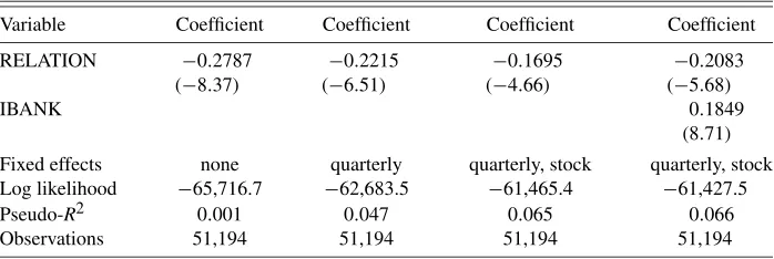
In Table3 we run an ordered logit model of recommenda-tions as a function of our conflict of interest measures. The co-efficient on RELATION indicates that potential conflicts of in-terest are statistically significant at conventional levels, except for the third column where quarterly and stock fixed effects are included, and the fourth column where the full set of fixed ef-fects are included along with the more inclusive IBANK vari-able. The coefficient sign on RELATION is also consistent with our a priori beliefs that conflicts of interest could lead to the issuance of more favorable recommendations. However, these results must be interpreted with some caution. Since brokerage firms are expected to cover companies with whom they have significant investment banking business, the firms have an in-centive to select brokerages that already view them favorably. It would be hard to imagine that a rational manager would want to hire an investment banking firm that views her company in an unfavorable manner.
Our results suggest that even though investment banking re-lationships may generate potential conflicts of interest for eq-uity analysts, the magnitude of the effects on recommendations
Table 3. Ordered logit estimates of the effect of conflicts of interest
Variable Coefficient Coefficient Coefficient Coefficient
RELATION −0.2787 −0.2215 −0.1695 −0.2083
(−8.37) (−6.51) (−4.66) (−5.68)
IBANK 0.1849
(8.71)
Fixed effects none quarterly quarterly, stock quarterly, stock Log likelihood −65,716.7 −62,683.5 −61,465.4 −61,427.5
Pseudo-R2 0.001 0.047 0.065 0.066
Observations 51,194 51,194 51,194 51,194
Table 4. Ordered logit estimates of peer effects (parametric first stage)
Variable Coefficient Coefficient Coefficient Coefficient
IVBELIEF 1.5937 1.5807 0.1437 0.1507
(71.33) (66.6) 2.98 3.2
RELATION −0.2036
(−4.84)
IBANK 0.1845
(8.16)
Fixed effects none stock quarterly, stock quarterly, stock Log likelihood −62,371.0 −62,078.4 −61,315.8 −61,267.9
Pseudo-R2 0.049 0.053 0.065 0.066
Observations 51,194 51,194 51,194 51,194
may be small in practice. Notice that measures of the goodness of fit are very low when only investment banking relationship is included. This overall finding is not consistent with the pros-ecutor’s belief that “unbiased” research, separate from invest-ment banking, will generate recommendations less tainted by potential conflicts of interest.
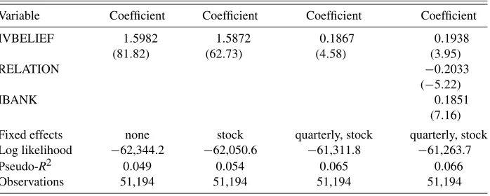
The final question we consider is whether peer effects come into play when analysts submit their recommendations. We ex-plore this question in Tables4–6 by using the two-stage pro-cedure described in the previous sections. First, we regress the recommendations on a broker fixed effect, a full set of stock and quarterly dummies, and IBANK. In Table4, these first-stage re-gressions are done using linear regression, while in the later ta-bles we include stock-time interactions as a more flexible first stage. We experimented with other functional forms, such as a 3rd-order spline, and the results were little changed. We will let IVBELIEF for an analyst-brokeridenote the expected aver-age recommendation from the first-staver-age model, where the av-erage excludes the predicted recommendation of that brokeri. If the coefficient on IVBELIEF is positive, this means that bro-kerihas an incentive to conform to the recommendations of the other brokers. If it is negative, it means there is a return from submitting a dissenting recommendation.
In all of the specifications that we examine in Table4, peer effects seem to be important. An individual analyst will raise his recommendation proportionally to the recommendation that he expects from other analysts. This is intuitive. A recommen-dation does not make sense in isolation, but only in comparison to the recommendations of other analysts. If no one else in the
market is issuing recommendations of “market underperform” or “sell,” an individual analysts may give the wrong signal by issuing such a recommendation even if he believes the recom-mendation is literally true. It is worth noting that the results for our measure of peer effects are not only statistically significant, but peer effects also explain the results quite well compared to the other covariates. The Pseudo-R2suggests that quarterly dummies, stock dummies, and IVBELIEF explain most of the variation in the data. Adding the additional conflict of interest variables does not do much to improving the model fit.
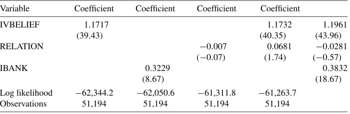
We note that the presence of the peer effect is robust to allow-ing for a more flexible first stage (see Tables5and6). Also, the peer effect remains significant, allowing for unobserved hetero-geneity in the form of a stock/quarter-specific random effect in Table6. For these specifications, the investment banking rela-tionship coefficient is no longer significant. In the random effect specification, the individual effect component is assumed to be drawn from a normal distribution with mean zero and a constant variance. The validity of the random effect model requires the strong assumption that the random effects are orthogonal to the regressors and the errors.
Note that it is possible to extend this analysis by using the parameter estimates obtained above and simulating the model in order to find all the equilibria in the recommendation game. Bajari et al. (2009) develop an algorithm to compute all so-lutions to this recommendation game (as well as to other ap-plications). Perhaps not surprisingly, we find evidence of two equilibria in the pre-Spitzer era, one of which was character-ized by an across-the-board tendency for analysts to grant more
Table 5. Ordered logit estimates of peer effects (semiparametric first stage)
Variable Coefficient Coefficient Coefficient Coefficient
IVBELIEF 1.5982 1.5872 0.1867 0.1938
(81.82) (62.73) (4.58) (3.95)
RELATION −0.2033
(−5.22)
IBANK 0.1851
(7.16)
Fixed effects none stock quarterly, stock quarterly, stock Log likelihood −62,344.2 −62,050.6 −61,311.8 −61,263.7
Pseudo-R2 0.049 0.054 0.065 0.066
Observations 51,194 51,194 51,194 51,194