Full Terms & Conditions of access and use can be found at
http://www.tandfonline.com/action/journalInformation?journalCode=ubes20
Download by: [Universitas Maritim Raja Ali Haji] Date: 12 January 2016, At: 23:03
Journal of Business & Economic Statistics
ISSN: 0735-0015 (Print) 1537-2707 (Online) Journal homepage: http://www.tandfonline.com/loi/ubes20
The Difference Between Hedonic Imputation
Indexes and Time Dummy Hedonic Indexes
Mick Silver & Saeed Heravi
To cite this article: Mick Silver & Saeed Heravi (2007) The Difference Between Hedonic Imputation Indexes and Time Dummy Hedonic Indexes, Journal of Business & Economic Statistics, 25:2, 239-246, DOI: 10.1198/073500106000000486
To link to this article: http://dx.doi.org/10.1198/073500106000000486
Published online: 01 Jan 2012.
Submit your article to this journal
Article views: 48
View related articles
The Difference Between Hedonic Imputation
Indexes and Time Dummy Hedonic Indexes
Mick S
ILVERStatistics Department, International Monetary Fund, Washington, DC 20431 (msilver@imf.org)
Saeed H
ERAVICardiff University, Business School, Cardiff CF10 3EU, U.K. (heravis@cf.ac.uk)
Statistical offices try to match item models when measuring inflation between two periods. However, for product areas with a high turnover of differentiated models, the use of hedonic indexes is more appro-priate, because these include the prices and quantities of unmatched new and old models. The two main approaches to hedonic indexes are hedonic imputation (HI) indexes and dummy time hedonic (DTH) in-dexes. This study provides a formal analysis of the difference between the two approaches for alternative implementations of the Törnqvist “superlative” index. It shows why the results of the HI and DTH indexes may differ and discusses the issue of choice between these two approaches.
KEY WORDS: Consumer price index; Hedonic index; Hedonic regression; Superlative indexes.
1. INTRODUCTION
The purpose of this article is to outline and compare the two main and quite distinct approaches to the measurement of he-donic price indexes: dummy time hehe-donic (DTH) indexes and hedonic imputation (HI) indexes, also referred to as “character-istic price index numbers” (Triplett 2004). Both approaches not only correct price changes for changes in the quality of items purchased, but also allow the indexes to incorporate matched and unmatched models. They provide a means by which price change can be measured in product markets where there is a rapid turnover of differentiated models; however, they can yield quite different results. This article provides a formal exposi-tion of the factors underlying such differences and the implica-tions for choice of method. This is undertaken for the Törnqvist index, a superlative formula. As explained, superlative index number formulas, which include the Fisher index, have desir-able properties and provide similar results.
The standard way in which price changes are measured by national statistical offices is through the matched-models method. In this method the details and prices of a representa-tive selection of items are collected in a base reference period and their matched prices are collected in successive periods so that the prices of “like” are compared with “like.” However, if there is a rapid turnover of available models, then the sample of product prices used to measure price changes becomes un-representative of the category as a whole. This is as a result of both new unmatched models being introduced but not included in the sample and older unmatched models being retired and thus dropping out of the sample. Hedonic indexes use matched and unmatched models, thereby avoiding the matched-models sample selection bias (see Cole et al. 1986; Silver and Heravi 2003, 2005; Pakes 2003). The need for hedonic indexes can be seen in the context of the need to reduce bias in the mea-surement of the U.S. consumer price index (CPI), which has been the subject of three major reports by the Stigler Committee (Stigler 1961), the Boskin Commission (Boskin 1996), and the Committee on National Statistics (2002) (the Schultze Panel). Each found the inability to properly remove the effect on price changes of changes in quality to be a major source of bias. He-donic regressions were considered the most promising approach
to control for such quality changes, although the Schultze Panel cautioned for the need for further research on methodology:
Hedonic techniques currently offer the most promising approach for explic-itly adjusting observed prices to account for changing product quality. But our analysis suggests that there are still substantial unresolved econometric, data, and other measurement issues that need further attention (Committee on Na-tional Statistics 2002, p. 6).
At first sight, the two approaches to hedonic indexes appear quite similar. Both rely on hedonic regression equations to re-move the effects on price of quality changes. They can also in-corporate a range of weighting systems; can be formulated as a geometric, harmonic, or arithmetic aggregator function; and as chained or direct, fixed-base comparisons. Yet they can give quite different results, even when using comparable weights and functional forms and the same periodic comparison. This is be-cause they work on different principles. The dummy variable method constrains hedonic regression parameters to remain the same over time. An HI index conversely relies on parameter change as the essence of the measure.
There has been some valuable research on the two ap-proaches (see Berndt and Rappaport 2001; Diewert 2002; Silver and Heravi 2003; Pakes 2003; de Haan 2004; Triplett 2004), al-though to the best of our knowledge no formal analysis of the factors governing the differences between the approaches has been published. Berndt and Rappaport (2001) and Pakes (2003) highlighted the fact that the two approaches can give different results, and both advise using HI indexes when parameters are unstable, a proposal considered in Section 4.
The article is organized as follows. Section 2 examines the al-ternative formulations of the two main methods, and Section 3 develops an expression for their differences. Section 4 discusses the issue of choice between the approaches in light of the find-ings, and Section 5 concludes.
In the Public Domain Journal of Business & Economic Statistics April 2007, Vol. 25, No. 2 DOI 10.1198/073500106000000486 239
240 Journal of Business & Economic Statistics, April 2007
2. HEDONIC INDEXES
A hedonic regression equation of the prices ofi=1, . . . ,N
models of a product,pi, on their quality characteristics zki,
wherezk=1, . . . ,Kprice-determining characteristics, is given
in a log-linear form by
Here theβk’s are estimates of the marginal valuations the data
ascribes to each characteristic (Rosen 1974; Griliches 1988; Triplett 1988; Diewert 2003; Pakes 2003). Statistical offices use hedonic regressions in CPI measurement when a model is no longer sold and a price adjustment for the quality difference is needed. This adjustment is done so that the price of the original model can be compared with that of a noncomparable replace-ment model. Silver and Heravi (2001) referred to this as “patch-ing.” However, only when a model is missing is a new replace-ment found, and this is on a one-to-one basis. In dynamic mar-kets, such as PCs, old models regularly leave the market and new ones are regularly introduced, not necessarily on a one-to-one basis. There is a need to incorporate the prices of all “unmatched” models of differing quality, andhedonic indexes
provide the required measures.
2.1 Hedonic Imputation Indexes
HI indexes take a number of forms: (1) as either equally weighted or weighted indexes; (2) depending on the functional form of the aggregator, say a geometric aggregator as against an arithmetic one; (3) with regard to which period’s character-istic set is held constant; and (4) as direct binary comparisons between periods 0 and t, or as chained indexes. For chained indexes, the individual links are calculated between periods 0 and 1, 1 and 2, . . . ,t−1 andt, and the results combined by successive multiplication.
We consider in this section, as (2) and (3), hedonic Laspeyres and Paasche indexes—weighted, arithmetic, constant base (Laspeyres) and current (Paasche) period, aggregators for bi-nary comparisons—and then, for the purposes of this article, focus on a generalized hedonic Törnqvist index, given by (4). The Törnqvist index is a weighted, geometric aggregator that makes symmetric use of base and current information in binary comparisons. It is a superlative index and thus has highly de-sirable properties. An index number is defined asexactwhen it equals the true cost of living index for a consumer whose pref-erences are represented by a particular functional form. A su-perlativeindex is defined as an index that is exact for a flexible functional form that can provide a second-order approximation to other twice-differentiable functions around the same point. Superlative indexes are generally symmetrical with respect to their use of information from the two time periods (see Diewert 2004). Fisher and Walsh index formulas are also superlative in-dexes and closely approximate the Törnqvist index. The Fisher index is the preferred target index in the international CPI man-ual (Diewert 2004, chaps. 15–18).
We start by outlining the hedonic formulations of the well-known Laspeyres and Paasche indexes. Consider the hedonic
functionpˆ0i =h0(z0i)from the semilogarithmic form of (1), es-timated in period 0 with a vector of K quality characteristics
z0i =z0i1, . . . ,z0iKandN0observations and similarly for period 1. Let quantities sold in periods 0 and 1 beq0i andq1i.
A hedonic Laspeyres index formatched and unmatched pe-riod0 models is given by
PHLas=
and a hedonic Paasche index formatched and unmatched pe-riod1 models is given by
PHPas=
It is apparent from (2) and (3) that a hedonic Laspeyres index holds characteristics constant in the base period and a hedo-nic Paasche index holds the characteristics constant in the cur-rentperiod. Thus the differences in hedonic valuations in the Laspeyres and Paasche indexes are dictated by the extent to which the characteristics change over time, that is,z1i −z0i. The more thezi values differ over time (due, say, to greater
tech-nological change), the less justifiable the use of an individual estimate and the less faith in a compromise geometric mean of the two indexes—a Fisher index. Note that new (unmatched) models available in period 1 but not in period 0 are excluded from (2) and that old (unmatched) models available in period 0 but not in period 1 are excluded from (3). The Laspeyres and Paasche HI indices suffer from a sample selectivity bias.
Leti∈St(t=0,1) be the set of models available in periodt. Leti∈SM≡S0∩S1 be the set of matched models with com-mon characteristicszmi =z0i =z1i in both periods 0 and 1. Un-matched new models present in period 1 but not in period 0 are given byi∈S1(1¬0), and unmatched old models present in period 0 but not in period 1 are given byi∈S0(0¬1). Let the number of models in these sets be denoted byNM,N0(0¬1), andN1(1¬0). A hedonic Törnqvist index, for matched mod-els only, is given by the first term on the right side of (4). The hedonic Törnqvist index isgeneralizedto include disappearing and new models by the respective inclusion of the second and third terms on the right side of (4). An alternative and equiva-lent formulation to (4) would be to include only these last two terms, but with the products taken overi∈S0andi∈S1. But, we use (4), because it provides a more detailed, and analytically useful, decomposition of the price changes of the different sets of models.
A generalized hedonic Törnqvist index is given by
PHTörnqvist= i∈S
where relative expenditure shares for model i in period t are given bysti=ptiqti/
jptjq t
jfort=0,1 and expenditure shares
for matched models m are an average of those in periods 0 and 1, that is,s˜mi =(s0i +si1)/2 fori∈SM. Note that˜smi (for
i∈SM) pluss0i/2 (fori∈S0(0¬1)) pluss1i/2 (fori∈S1(1¬0))
sum to unity. For illustration, if the expenditure shares of matched models were .6 in period 0 and .7 in period 1, that of unmatched old models was .4 in period 0, and that of unmatched new models was .3 in period 1, then
i˜smi =.65,
is0i/2=.2,
and
is1i/2=.15.
Note that estimated prices are used for matched models. A good case can be made for using actual prices for matched models when available (de Haan 2004).
Equation (4) is a (superlative) Törnqvist HI index general-ized to include new and disappearing models. In Section 2.2 a DTH index is identified as an alternative approach to estimat-ing a generalized Törnqvist hedonic index. The issue addressed here is identifying an expression for the differences between the HI and DTH approaches. As we discuss, an econometric device is useful in this respect, which requires that we work with pre-dicted, rather than actual, prices for matched models, although this article is not alone in this (see Pakes 2003).
2.2 Dummy Time Hedonic Indexes
DTH indexes provide an approach to estimating price changes that use hedonic regressions to control for the differ-ent quality mix of new and disappearing models. As with HI indexes, DTH indexes do not require a matched sample. In this section we show how the generalized Törnqvist hedonic index in (4) can be estimated as a DTH index. The DTH formulation is similar to (1), except that a single regression is estimated on the data in the two time periods, 0 and 1 compared,i∈St for
t=0,1. The prices, pti, for each modeli are regressed on a dummy variable,Dt0i, that is equal to 1 in period 1 and 0 other-wise, andztki=1, . . . ,Kprice-determining characteristics in a regression with well-behaved residuals,εit,
lnpti=δ0+δ1Dt0i+ K
k=1
βkztki+ε t
i fori∈Standt=0,1. (5)
The exponent of the estimated coefficient δ1∗ is an estimate of the quality-adjusted price change between periods 0 and 1 regardless of the reference quality vector. Consider, for sim-plicity, the case of only matched models where there is no need for the quality characteristics, ztki, in (5). Then δ∗1 =
1/nn
i=1(lnp1i −lnp0i)and exp(δ1∗)is the geometric mean of
p1i/p0i—with an adjustment, as detailed by van Garderen and Shah (2002). Also note that for unmatched models, because
βk0=βk1=βk in (5), the value ofδ1∗ is invariant to the level
ofztki; the lines of the functions of lnptionztkifor periodst=0,1 are parallel, and the shift intercept is constant.
It first may be thought that weighted indexes such as the tar-get Törnqvist index cannot be compared with DTH indexes, as in (5), because the latter are unweighted (equally weighted). However, Diewert (2002, 2005) showed that if a weighted least squares (WLS) estimator is applied to (5), then the resulting estimate of price change will correspond to a weighted index number formula. More specifically, formulation of the weights for the WLS estimator dictates which index number formula the DTH estimate corresponds with. A WLS estimator is equivalent to an ordinary least squares (OLS) estimator applied to data that have been repeated in line with their weight, akin to repeated sampling. A DTH price change estimate as given by (5) and based on a WLS estimator, with weightss˜mi =(s0i +s1i)/2 for matched models and s0i/2 for unmatched old models ors1i/2 for unmatched new models, corresponds to a generalized Törn-qvist index (Diewert 2005). In Section 3.1 we use this weight-ing structure to derive and compare generalized DTH and HI Törnqvist index estimates.
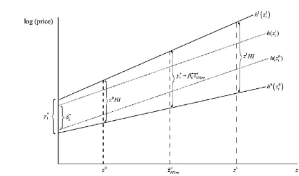
The regression equation (5) constrains each of theβk
coeffi-cients to be the same across the two periods compared. In re-stricting the slopes to be the same, the (log of the) price change between periods 0 and 1 can be measured at any value ofz, as il-lustrated by the difference between the dashed lines in Figure 1. For convenience, it is first evaluated at the origin asδ1∗. Bear in
Figure 1. Depiction of difference between hedonic imputation and dummy time hedonic indices.
242 Journal of Business & Economic Statistics, April 2007
mind that the HI indexes outlined earlier estimate the differ-ences between price surfaces with different slopes. As such, the estimates must be conditioned on particular values ofz, which gives rise to the two estimates (whose arithmetic equivalents are) considered in (2) and (3): the base HI usingz0and the cur-rent period HI usingz1, as shown in Figure 1. The very core of the DTH method is to constrain the slope coefficients to be the same, so there is no need to condition on particular values ofz. The DTH estimates implicitly and usefully make symmetric use of base and current period data. As with HI indexes, DTH in-dexes can take fixed and chained base forms, and can also take a fully constrained form whereby a single constrained regression is estimated for, say, January to December with dummy vari-ables for each month, although this is impractical in real time because it requires data on future observations.
3. WHY HEDONIC IMPUTATION AND DUMMY TIME HEDONIC INDEXES DIFFER
3.1 Algebraic Differences: A Reformulation of the Hedonic Indexes
There has been little analytical work undertaken on the fac-tors governing differences between the two approaches. To compare the HI and DTH approaches, we first need to refor-mulate the HI indexes. We note that the HI approach relies on two estimated hedonic equations,h1(z1i)andh0(z0i), for periods
We assume that the errors in each equation are similarly distrib-uted, then phrase the two equations as a single hedonic regres-sion equation with dummy time intercept and slope variables,
lnpti=γ00+γ1Dt0i+
whereDt0i=1 if observations are in period 1 and 0 otherwise,
γ1=(γ01−γ00),Dtki=z1kiif observations are in period 1 and 0 otherwise, and βk =(βk1−βk0). The estimatedγ1∗ is an
esti-mate of the change in the interceptsof the two hedonic price equations and thus is an HI index evaluated at a particular value ofztki,i∈St andt=0,1; let this value be denoted byz˜tkwhich is equal to 0 at the intercept. An HI index evaluated atz˜tk=0 has no economic meaning.
For our phrasing of a HI index in (10) to correspond to the generalized hedonic Törnqvist index in (4) requires two condi-tions. First, a WLS estimator should be used to estimateγ1from (8) with weights˜smi =(s0i +s1i)/2 for matched models ands0i/2 for unmatched old models ors1i/2 for unmatched new models (Diewert 2002, 2005). Second, the estimate ofγ1 in (8) is at
the intercept, whereas the generalized HI Törnqvist index (4) requires that it be evaluated at a mean value ofztkigiven by
˜
For a Törnqvist HI index, the γ1∗ estimate is evaluated at
˜
ztk= ¯ztkTörn. This requires an adjustment to theγ1∗estimate. The required generalized HI Törnqvist index is given by the exponent of
Consider now the DTH index in (5) that constrains βk =
βk1−βk0=0 in (8) and thus K
k=1βkDki to be 0. The DTH
index in (5) corresponds to a generalized DTH Törnqvist index if estimated using WLS where the weights are those outlined after (5). A natural question is how does the estimated DTH in-dexδ1∗in (5), which is invariant to values ofztki, differ from the HI index evaluatedat the mean,¯ztkTörn, in (10)?
3.2 How Does a Törnqvist Hedonic Imputation Index Differ From a Törnqvist Dummy Time
Hedonic Index?
This difference is first considered by comparingγ1∗from (8), the HI index, andδ1∗from (5), the DTH index. We are interested in the difference in these two estimatedinterceptshifts, where
˜
ztk=0, between the estimated constant-quality shift parameters from the constrained (DTH) and unconstrained (HI) regression equations (5) and (8). Being intercept shifts, the difference be-tween these two indexes will be determined at the origin, where
˜
ztk=0. This is useful as a first stage in the derivation. However, we then extend the analysis to examine how the expressions differ at, more usefully, the meanz¯tkTörnfrom (9). We now turn to a consideration of the differenceδ∗1−γ1∗between these two dummy variable parameter estimates at the origin, as “omitted variable bias” due to the omission ofK
k=1βkDkiin (8).
Expressions for the bias in estimated regression parame-ters due to the omission of relevant variables are well estab-lished (see Maddala 1992, pp. 161–163). For example, the bias for a parameter estimate ofβ1 in a regression equation,
y=β0+β1x1+β2x2+u, from a regression that excludesx2 is equal to the coefficient on the excluded variable,β2, multi-plied by the coefficient on the included variable,α1, from an auxiliary regression of the excluded on the included variable, that is,x2=α0+α1x1+ω. Consider a simplified case of (8) of a singlek=1 characteristic and two time periods, with the principles being readily extended. The auxiliary regression is the slope dummy variable,Dt1i [=z11i if period 1 and 0 other-wise, in (8)], regressed on the remaining right side variables in (8), the intercept dummyDt0i, and thezt1icharacteristic with
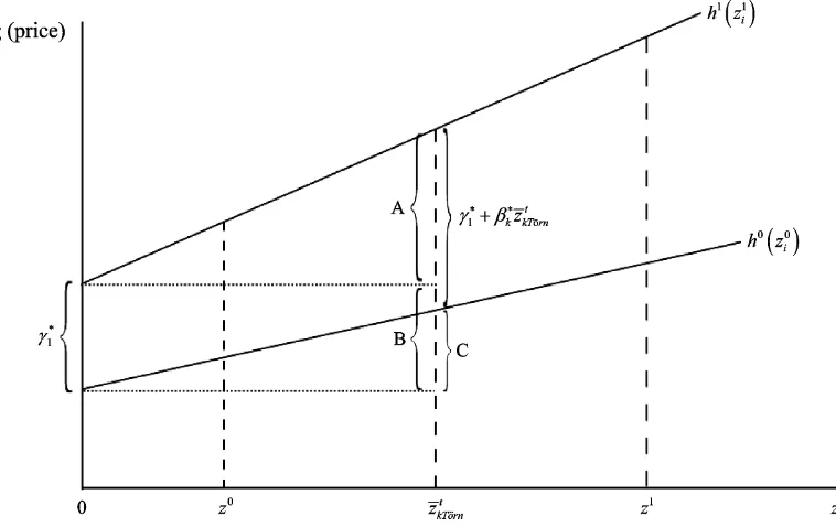
Figure 2. The Required Estimate Is Depicted as the Vertical Difference Between the Two Hedonic Functions, h1(zi1) and h0(zi0) at a Com-monz¯k Tt orn¨ . This is given by A+B−C. A isβ1z¯kTt orn¨ , whereβ1is the slope of h1(zi1); B is estimated byγ1∗; and C is estimated byβ0z¯tkTorn¨ , whereβ0is the slope of h0(zi0). A+B−C is estimated byγ1∗+βk∗z¯kTt orn¨ , whereβk∗is a WLS estimate ofβ1k−βk0and (10) generalizes this for more than one k .
Omitted variable bias is the product of the estimated coefficient on the omitted variable,β1∗[fork=1 in (8)], and the estimated coefficientλ∗1from regression (11) (Maddala 1992). Thus the difference (before taking exponents) DTHminusHIat the in-terceptisδ1∗−γ1∗=β1∗×λ∗1.
Our next concern is to derive this difference atz¯t1Törnrather than atz˜tk=0. Because the DTH method holds the parameter estimates constant through any value ofztk, the (log of the) DTH index is given byδ∗1=β1∗×λ∗1+γ1∗. However, the (log of the) Törnqvist HI index at¯zt1Törn from (8) for one variable is esti-mated as
γ1∗+β1∗¯zt1Törn. (12) Thus the ratio of the DTH and HI indexes at the intercept is exp(δ1∗)/exp(γ1∗)=exp(β1∗×λ∗1), and thus the DTH index is given by exp(δ∗1)=exp(β1∗×λ∗1)×exp(γ1∗). The Törnqvist HI index at z¯t1Törn from (8) for one variable is estimated as exp(γ1∗+β1∗¯zt1Törn). Thus the ratio of the Törnqvist DTH index to the Törnqvist HI index at¯zt1Törnis
Törnqvist DTH index Törnqvist HI index
.. .¯zt1Törn
=exp (β1∗1−β1∗0)(λ∗1− ¯zt1Törn), (13)
whereβ1∗1andβ1∗0are WLS estimates.
If either of the two terms composing the product on the right side is close to 0, then there will be little difference between the indexes. Neither parameter instability nor a change in the mean characteristic is sufficient in itself to lead to a differ-ence between the formulas. The β1∗=βk∗1−βk∗0 from (5) is the estimated marginal valuation of the characteristic between periods 0 and 1, which can be positive or negative, but may be more generally considered negative to represent diminishing marginal utility/cost of the characteristic.
3.3 Interpretation of (λ∗1− ¯z1Törnt )
Equation (13) shows that the change in the coefficients is one factor determining the differences between the two methods. The second expression,(λ∗1− ¯zt1Törn), is more difficult to inter-pret, and we consider it here. Bear in mind that the left side of the regression in (11),Dt1i, is 0 in period 0 andz11i in period 1 and thatDt0ion the right side is 1 in period 1 and 0 in period 0. If we assume quality characteristics are positive,λ1will always be positive as the change from 0 in period 0 to their values in period 1. Consider the weighted (Törnqvist) mean ¯z01Törn for
i∈SM andi∈S0(0¬t)(matched period 0 and unmatched old period 0) and ¯z11Törn fori∈SM andi∈St(1¬0)(matched pe-riod 1 and unmatched in pepe-riod 1).
If we assume for simplicity that z¯01Törn = ¯z11Törn, then
λ∗1≈ ¯z11Törn, becauseλ∗1 is an estimate of the change inDt1i in (11) arising from changing from period 0 to period 1, where it is ¯z11Törn and has an expectation of z¯11Törn. The λ∗1 esti-mate is conditioned in (11) onz¯t1Törn, the change from ¯z01Törn
to ¯z11Törn, but because we assume that these two have not changed, our estimate ofλ∗1≈ ¯z11Törnholds true. Thus the sec-ond part of the difference expression in (13), (λ∗1− ¯zt1Törn), is simply (z¯11Törn− ¯zt1Törn), which, given our assumption of
¯
z01Törn= ¯z11Törn, is equal to 0. It follows from the right side of (13) that for samples with negligible change in the mean values of the characteristics, the DTH and HI will be similar irrespective of any parameter instability. Diewert (2002) and Aizcorbe (2003) have shown that the DTH and HI indexes will be the same for matched models, and the present analysis gives support to their findings. However, we find first that it is not matching per se that dictates the relationship; for unmatched models all that is required is that z¯11Törn= ¯zt1Törn, which may
244 Journal of Business & Economic Statistics, April 2007
occur without matching—it simply requires that the means of the characteristics not change. Second, even when the means change, the two approaches will be equal if βk∗1−βk∗0=0, that is, there is parameter stability. Finally, it follows that if ei-ther of the two right-side expressions in (13) are large, then the differences between the indexes are compounded.
But what if ¯z01Törn= ¯z11Törn? Because the estimated coef-ficient on x1 of a regression of y on x1 and x2 is given by
(
yx1x22−yx2x1x2)/(x21x22−(x1x2)2), the estimated coefficientλ∗1from (11) is given by
λ∗1=z¯
for an unweighted regression, where N1 and N are the re-spective number of observations in period 1 and both peri-ods 0 and 1, σz2 is the variance of z, and cov(D1ti,zt1i)=
(zt)2−N1z¯1z¯ is the covariance of Dt1i and zt1i from (11). Keep in mind that, from (13),
First, as noted earlier, if there is either negligible parameter in-stability or a negligible change in the mean of the character-istic, then there will be little difference between the formulas. However, as parameter instability increases and the change in the mean characteristic increases, the multiplicative effect on the difference between the indexes is compounded. The likely direction and magnitude of any difference is not immediately obvious. Assume diminishing marginal valuations of character-istics, so that β1∗1−β1∗0<0. Second, even assuming a posi-tive technological advance,¯z11− ¯zt1>0, and given thatN−N1, cov(Dt1i,zt1i),¯z11, andσz2are positive, it remains difficult to es-tablish from (14) the effect onλ∗1of changes in its constituent parts. But third, asN1becomes an increasing share ofN, and at the limit if N1 takes up all ofN [i.e., N−N1→0], then cov(Dt1i,zt1i)→σz2 and, importantly,z¯11→ ¯zt1, and the differ-ence between the formulas tends to 0. Note that (14) is based on an OLS estimator and for a WLS Törnqvist estimator sim-ilar principles apply, though the determining factor for a DTH index to exceed a HI index is for the weights of new models to be increasing, a much more reasonable scenario. Thus the na-ture and extent of any differences between the two indexes will, aside from the parameter change, also depend on (a) changes in the mean quality of models,z¯11− ¯zt1; (b) the relative number
Diewert (2002) and Aizcorbe (2003) showed that although the DTH and HI indexes are the same for matched models, they differ in their treatment of unmatched data. Consider hedonic functionsh1i(z1i)andh0i(z0i)for periods 1 and 0 as in (2) and (3)
and a (constrained) time dummy regression equation (5). Con-sider further an unmatched observation available only in pe-riod 1. A base pepe-riod HI index such as (2) would exclude it, whereas a current period HI index, such as (3), would include it, and a geometric mean of the two would give it half the weight in the calculation of that of a matched observation. A Törnqvist hedonic index, (4), would also give an unmatched model half the weight of a matched one. For a DTH index, such as (5), an unmatched period 1 model would appear only once in period 1, in the estimation of constrained parameters, as opposed to twice for matched data. We thus would expect superlative HI indexes, such as (4), to be closer to DTH indexes than their constituent elements, (2) and (3), because they make symmetric use of the data.
3.5 Observations With Undue Influence
HI indexes, such as (2) and (3), explicitly incorporate weights. Silver (2002) and Diewert (2005) have shown that weights are implicitly incorporated in DTH indexes by means of the OLS or WLS estimator used. Silver (2002) has further shown that for DTH indexes, the manner in which the esti-mator incorporates the weights may not fully represent the weights, due to adverse influence and leverage effects generated by observations with unusual characteristics and above-average residuals.
3.6 Chaining
Chained-base HI indexes are preferred to fixed-base in-dexes, especially when matched samples degrade rapidly. In such a case, their use reduces the spread between Laspeyres and Paasche indexes. However, caution is advised when us-ing chained monthly series when prices may oscillate around a trend (i.e., “bounce”); as a result, chained indexes can “drift” (Forsyth and Fowler 1981; Szulc 1983).
4. CHOOSING BETWEEN HEDONIC INDEXES AND TIME DUMMY HEDONIC INDEXES
The main concern with the DTH index approach as given by (5) is that by construction, it constrains the parameters on the characteristic variables to be the same. The HI indexes have no such constraint. For example, Berndt and Rappaport (2001) found that from 1987 to 1999 for desktop PCs, the null hypoth-esis of adjacent-year equality was rejected in all cases but one. For mobile PCs, the null hypothesis of parameter stability was rejected in 8 of the 12 adjacent-year comparisons. Berndt and Rappaport (2001) preferred using HI indexes if there was ev-idence of parameter instability. Pakes (2003), using quarterly data for hedonic regressions for desktop PCs over 1995–1999, rejected just about any hypothesis on the constancy of the co-efficients. He also advocated HI indexes on the grounds that “. . . since hedonic coefficients vary across periods, it [the DTH index approach] has no theoretical justification” (Pakes 2003, p. 1593).
The concern about parameter instability for DTH methods is warranted. Consider constraining the estimated coefficients in a DTH index to eitherβ1∗1 or β1∗0, the index is likely to give
quite different results, and this difference is a form of “spread.” A DTH index constrains the parameters to be the same, an av-erage of the two. There is a sense in which we have more con-fidence in an index based on constraining similar parameters than one based on constraining two disparate parameters. Equa-tion (15) showed that β1∗1−β1∗0 was a determining factor in the nature and magnitude of any difference between the HI and DTH indexes.
However, (15) also showed how the ratio of DTH and HI indexes was not solely dependent on parameter instability. In-stead, it depended on the exponent of the product of two com-ponents: the change over time in the (WLS-estimated) hedonic coefficients and the difference in (statistics that relate to) the (weighted) mean values of the characteristic. Even if parame-ters are unstable, the difference between the indexes may be compounded or mitigated by a change in the other component.
Note that base and current period HI indexes, (2) and (3), can differ as a result of using a constantz1i as against a constantz0i. Diewert (2002) has argued that HI indexes have the disadvan-tage in that two distinct estimates will be generated, and it is somewhat arbitrary how these two estimates are to be averaged to form a single estimate of price change. Of course, Diewert (2003) also resolved this very problem by considering superla-tive hedonic indexes, that is, by using not just the base or just the current period characteristic configurations, but a symmetric average such as (4).
Nonetheless, there is a sense that in constraining the coeffi-cients to be the same, the DTH index performs a similar aver-aging function, but with the parameter estimates. Rather than using a base or current period coefficient set, it constrains them to form an average. There is then the question of which form of constraint is preferred: averaging the characteristic set (HI) or the coefficients (DTH)?
There is much in the theory of superlative index numbers that argues for taking a symmetric mean of the characteristic quantities or value shares. The result is that HI indexes fall more neatly into existing index number theory. At least in this sense they are to be preferred, although (15) provides useful insights into their differences compared with DTH indexes.
5. CONCLUSIONS
It is recognized that extensive product differentiation with a high model turnover is an increasing feature of product mar-kets (Triplett 1999). The motivation of this article lay in the failure of the matched models method to adequately deal with price measurement in this context and the need for hedonic indexes as the most promising alternative (Committee on Na-tional Statistics, 2002). The article first developed, in Section 2, a Törnqvist generalized, hedonic index, that is, a Törnqvist in-dex number formula generalized to deal with matched and un-matched models and using hedonic regressions to control for quality changes. The article next considered HI and DTH in-dexes as the two main approaches to estimating a Törnqvist hedonic index. That the two approaches can yield quite differ-ent results is of concern. Section 3 provided a formal exposi-tion of the factors underlying the difference between the two approaches. It was shown that differences between the two ap-proaches may arise from both parameter instability and changes
in the characteristics, and that such differences are compounded when both occur. It further showed that similarities between the two approaches resulted if there was little difference in either component.
In Section 4, the choice between the two approaches was based on minimizing parameter instability as a concept of spread. The analysis led to the advice that either the DTH or HI index approach is acceptable if either the parameters are relatively stable or the values of the characteristic set do not change much over time; otherwise, HI indexes are preferred when there is evidence of parameter instability. Superlative for-mulations, such as the Törnqvist HI index, are well grounded in index number theory and considered preferable to the DTH in-dex constraining the parameters to be the same, for which there is less obvious justification.
ACKNOWLEDGMENTS
The authors acknowledge useful comments from Ernst Berndt (MIT), Erwin Diewert (University of British Columbia), Kevin Fox (UNSW), and two anonymous referees. Jan de Haan (Statistics Netherlands) provided particularly useful advice on the weighting system used.
[Received July 2004. Revised June 2006.]
REFERENCES
Aizcorbe, A. (2003), “The Stability of Dummy Variable Price Measures Ob-tained From Hedonic Regressions,” mimeo, Federal Reserve Board, Wash-ington, DC.
Berndt, E. R., and Rappaport, N. J. (2001), “Price and Quality of Desktop and Mobile Personal Computers: A Quarter-Century Historical Overview,”
American Economic Review, 91, 268–273.
Boskin, M. S. (Chair), Advisory Commission to Study the Consumer Price dex (1996), “Towards a More Accurate Measure of the Cost of Living,” In-terim Report to the Senate Finance Committee, Washington, DC.
Cole, R., Chen, Y. C., Barquin-Stolleman, J. A., Dulberger, E., Helvacian, N., and Hodge, J. H. (1986), “Quality-Adjusted Price Indexes for Computer Processors and Selected Peripheral Equipment,” Survey of Current Busi-nesses, 66, 41–50.
Committee on National Statistics (2002),At What Price? Conceptualizing and Measuring Cost-of-Living and Price Indexes, Washington, DC: National Academy Press.
de Haan, J. (2003), “Time Dummy Approaches to Hedonic Price Measure-ment,” paper presented at the Seventh Meeting of the International Work-ing Group on Price Indices, May 27–29, 2003, INSEE, Paris; available at
http://www.ottawagroup.org/meet.shtml.
(2004), “Hedonic Regressions: The Time Dummy Index as a Special Case of the Törnqvist Index, Time Dummy Approaches to Hedonic Price Measurement,” paper presented at the Eighth Meeting of the International Working Group on Price Indices, August 23–25, 2004, Helsinki, Finland; available athttp://www.ottawagroup.org/meet.shtml.
Diewert, W. E. (2002), “Hedonic Regressions: A Review of Some Unresolved Issues,” mimeo, University of British Columbia, Dept. of Economics.
(2003), “Hedonic Regressions: A Consumer Theory Approach,” in
Scanner Data and Price Indexes, eds. M. Shapiro and R. Feenstra, Chicago: University of Chicago Press, pp. 317–348.
(2004),Consumer Price Index Manual: Theory and Practice, Geneva: International Labour Office, chaps. 15–18.
(2005), “Weighted Country Product Dummy Variable Regressions and Index Number Formulas,”Review of Income and Wealth, 51, 561–570. Forsyth, F. G., and Fowler, R. F. (1981), “The Theory and Practice of Chain
Price Index Numbers,”Journal of the Royal Statistical Society, Ser. A, 144, 224–247.
Griliches, Z. (1988), “Postscript on Hedonics,” inTechnology, Education, and Productivity, ed. Z. Griliches, New York: Basil Blackwell, pp. 119–122. Maddala, G. S. (1992),Introduction to Econometrics, New York: Macmillan.
246 Journal of Business & Economic Statistics, April 2007
Pakes, A. (2003), “A Reconsideration of Hedonic Price Indexes With an Appli-cation to PCs,”The American Economic Review, 93, 1576–1593.
Rosen, S. (1974), “Hedonic Prices and Implicit Markets: Product Differentia-tion and Pure CompetiDifferentia-tion,”Journal of Political Economy, 82, 34–49. Silver, M. (2002), “The Use of Weights in Hedonic Regressions: The
Measure-ment of Quality-Adjusted Price Changes,” mimeo, Cardiff University Busi-ness School.
Silver, M., and Heravi, S. (2001), “Scanner Data and the Measurement of Infla-tion,”The Economic Journal, 11, 384–405.
(2003), “The Measurement of Quality-Adjusted Price Changes,” in
Scanner Data and Price Indexes, eds. M. Shapiro and R. Feenstra, Chicago: University of Chicago Press, pp. 277–317.
(2005), “A Failure in the Measurement of Inflation: Results From a Hedonic and Matched Experiment Using Scanner Data,”Journal of Business & Economic Statistics, 23, 269–281.
Stigler, G. (1961), “The Price Statistics of the Federal Government,” report to the Office of Statistical Standards, Bureau of the Budget, National Bureau of Economic Research.
Szulc, B. J. (1983), “Linking Price Index Numbers,” inPrice Level Measure-ment, Ottawa: Statistics Canada, pp. 537–566.
Triplett, J. E. (1988), “Hedonic Functions and Hedonic Indexes,” inThe New Palgraves Dictionary of Economics, Macmillan, pp. 630–634.
(1999), “The Solow Productivity Paradox: What Do Computers Do to Productivity?”Canadian Journal of Economics, 32, 309–334.
(2004),Handbook on Hedonic Indexes and Quality Adjustments in Price Indexes, Paris: Directorate for Science, Technology and Industry, OECD.
van Garderen, K. R., and Shah, C. (2002), “Exact Interpretation of Dummy Variables in Semi-Logarithmic Equations,”Econometric Journal, 5, 149–159.