Full Terms & Conditions of access and use can be found at
http://www.tandfonline.com/action/journalInformation?journalCode=ubes20
Download by: [Universitas Maritim Raja Ali Haji] Date: 12 January 2016, At: 23:03
Journal of Business & Economic Statistics
ISSN: 0735-0015 (Print) 1537-2707 (Online) Journal homepage: http://www.tandfonline.com/loi/ubes20
Intrinsic Bayesian Estimation of Vector
Autoregression Impulse Responses
Shawn Ni, Dongchu Sun & Xiaoqian Sun
To cite this article: Shawn Ni, Dongchu Sun & Xiaoqian Sun (2007) Intrinsic Bayesian Estimation of Vector Autoregression Impulse Responses, Journal of Business & Economic Statistics, 25:2, 163-176, DOI: 10.1198/073500106000000378
To link to this article: http://dx.doi.org/10.1198/073500106000000378
Published online: 01 Jan 2012.
Submit your article to this journal
Article views: 49
View related articles
Intrinsic Bayesian Estimation of Vector
Autoregression Impulse Responses
Shawn N
IDepartment of Economics, University of Missouri, Columbia, MO 65211 (NI@missouri.edu)
Dongchu S
UNDepartment of Statistics, Virginia Tech, Blacksburg, VA 24061
Xiaoqian S
UNDepartment of Statistics, University of Missouri, Columbia, MO 65211
We propose an information-theoretic alternative to the conventional Bayesian posterior mean estimator of impulse responses in vector autoregression (VAR) models. The proposed estimator is based on the in-trinsic entropy loss function, which is invariant to nonlinear transformations of parameters. Consequently, intrinsic estimation of impulse responses is equivalent to that of VAR parameters. The Bayesian estimator under the entropy loss involves a frequentist expectation of regressors. We propose Markov chain Monte Carlo algorithms to simulate the posterior of the frequentist expectation of regressors and compute the Bayesian estimates. We estimate the VAR impulse responses in two applications.
KEY WORDS: Bayesian vector autoregression; Entropy loss; Latent variables; Markov chain Monte
Carlo.
1. INTRODUCTION
In applications of vector autoregression (VAR) models, re-searchers are often more interested in inferences of impulse responses, which are nonlinear functions of VAR parameters, than of VAR parameters themselves. The Bayesian approach has been effective for finite-sample inferences of impulse re-sponses (e.g., see Sims 1980; Sims and Zha 1998). Although posterior distributions of quantities of interest are the ulti-mate result of Bayesian analysis, they are difficult to report in multiple-parameter settings. Therefore, Bayesian estimation of impulse responses is useful in summarizing the posterior for economic policy making. In Bayesian estimation of im-pulse responses, the default estimator is the posterior mean. In this article we propose an alternative Bayesian estimator based on an information-theoretic argument. We derive the proposed estimator and conduct Markov chain Monte Carlo (MCMC) simulations for Bayesian estimations in macroeco-nomic applications.
In what follows we provide an information-theoretic argu-ment for using the intrinsic loss function for Bayesian analysis. For a parameterθ, a Bayesian estimatorθ minimizes the pos-terior expected loss L(θ , θ ), whereθ denotes an estimator in general and an estimator under a particular loss. The estimator depends on the choice of loss function; for example, the pos-terior mean estimator is optimal ifL(θ,θ )is a quadratic loss function. On the principle of Bayesian estimation, Bernardo and Juárez (2003, p. 465) pointed out that
In practise, in most situations where point estimation is of interest, an objective point estimation is actually required: objective in the very precise sense of ex-clusively depending on the assumed probability model (i.e., on the conditional distribution of the data given the parameters) and the available data. Moreover, in purely inferential settings (where interest focuses on the actual mechanism which governs the data) this estimate is typically required to be invariant under one-to-one transformation of either the data or the parameter space.
They argued that the loss function should not concern a distance between θ and θ; instead, it should be the intrin-sic discrepancy,L{f(x|θ ),f(x|θ )}, the distance between the
probability models f(x|θ )andf(x|θ ). Bernardo and Juárez (2003) and Robert (1994, 1996) proposed using the logarithmic divergence (also known as the Kullback–Leibler divergence, or the entropy loss) as the intrinsic loss. The intrinsic loss is invari-ant to transformation of dataxor parameterθ. Suppose that the subject of interest is a one-to-one transformation of parameter α=ϕ(θ )instead ofθ itself; then the intrinsic loss with respect toαis equivalent to that with respect toθ.
In a VAR setting, intrinsic estimation of impulse responses is advisable. By definition, impulse responses are nonlin-ear functions of the VAR regression coefficients (represented byBhereinafter) and the covariance matrix (represented by
hereinafter) of the VAR error term. The most commonly used VAR impulse responses to orthogonal shocks are based Cholesky decomposition of, which depends on the ordering of variables. Koop, Pesaran, and Potter (1996) and Pesaran and Shin (1998) proposed generalized impulse responses, which are nonlinear functions ofandBas well, but independent of variable ordering. For many empirical applications, both types of impulse responses may be of interest. When we report the posterior mean of the impulse responses, we in effect make a statement on our best estimate of them with respect to a met-ric of quadratic distance. However, the VAR parameters (,B) corresponding to the posterior mean of impulse responses are not the posterior mean of (,B), our best estimate based on the quadratic loss. Reporting the posterior mean estimates of gener-alized impulse responses and those of impulse responses to or-thogonal shocks amounts to giving different sets of assessment on the values of the underlying VAR parameters. Intrinsic esti-mation under the entropy loss avoids this pitfall. Because there is a one-to-one mapping between the VAR parameters (,B) and impulse responses, estimation of (,B) is equivalent to
© 2007 American Statistical Association Journal of Business & Economic Statistics April 2007, Vol. 25, No. 2 DOI 10.1198/073500106000000378 163
estimation of the VAR impulse responses. In other words, the Bayesian estimators of impulse responses coincide with the im-pulse response functions of the Bayesian estimators of VAR parameters.
In this article we provide analytical as well as empirical results on the Bayesian estimator of VAR impulse responses under the entropy loss. We useto denote the intercept vec-torcand coefficient matrixB. We show that the entropy loss on (,) is nonseparable in and , which can be writ-ten as the sum of losses pertaining to the covariance matrix
(a pseudo–entry loss) and normalized estimation error of , with the weighting matrix being the frequentist expectation of a nonlinear function of regressors.
Besides the invariance property, the functional form of in-trinsic loss function just described lends support to its use. The part of the loss function associated with can be viewed as quadratic with a weighting matrix that depends on ,, and data. In particular, thepart of the loss is the estimation error inweighted by its contributions to the normalized estimate errors of residuals. This is in the spirit of Zellner’s “precision of the estimation” loss. Under the widely used quadratic loss, esti-mation errors in elements ofare weighted by constants, and the weights do not reflect the contribution of the estimation er-rors in coefficient to the estimation erer-rors of the residuals (i.e., the estimation errors of the overall model); in contrast, they do so under the intrinsic loss function.
To intuitively illustrate how the intrinsic loss function weighs the estimation error, we consider a simple AR(1) model, yt =ρyt−1+ǫt, for t =1, . . . ,T, where ǫt is iid N(0,1),
y0=0, and ρ is the only unknown parameter. Under a flat prior, the posterior of ρ given data yD is a normal distri-bution, N(ρM, (Tt=1y2Dt−1)−1). The posterior mean ρM is the maximum likelihood estimator (MLE),(Tt=1yDtyDt−1)×
(Tt=1y2Dt−1)−1.It is well known thatρM is biased downward, especially when the true parameter is close to unity (see MacKinnon and Smith 1998). For the AR(1) model with nor-mal densityf, the entropy loss isL(ρ, ρ) =log{f(y|ρ)/f(y|
ρ)}f(y | ρ)dy = (ρ−2ρ)2δ(ρ), where δ(ρ)=Ey|ρTt=1y2t−1. Under the entropy loss, the Bayesian estimator for ρ isρE= arg minE[δ(ρ)(ρ−ρ)2|yD] =E{δ(ρ)ρ|yD}/E{δ(ρ)|yD}. Note that ifρ is positive, thenρ andδ(ρ)are positively corre-lated. It follows that the Bayes estimator under the entropy loss for positiveρis always larger than the posterior mean.
The intrinsic estimator has a theoretically appealing inter-pretation. Note that the entropy loss can be viewed as the weighted squares of estimation errorρ−ρ. The weightδ(ρ)is Ey|ρTt=1y2t−1, the frequentist expectation of theposterior
pre-cision. The functional form means that the intrinsic loss func-tion penalizes estimafunc-tion errors more severely in the region whereρ is likely to generate data that give rise to high pos-terior precision. The quadratic loss, on the other hand, imposes a constant weight on all regions ofρ.
The rest of the article is organized as follows. In Section 2 we derive the Bayesian VAR estimator under the entropy loss func-tion. We show that the Bayesian estimator for is larger than the posterior mean. The Bayesian estimator for, which is also different from the posterior mean, involves frequentist moments of VAR variables. In Section 3 we discuss priors and prove the
existence of posterior moments pertaining to the Bayesian es-timator. In Section 4 we discuss several MCMC algorithms for posterior simulation. In Section 5 we estimate VAR impulse re-sponses in two applications on the U.S. macroeconomic data. In Section 6 we give some concluding remarks.
2. THE ENTROPY LOSS FUNCTION AND BAYESIAN ESTIMATION
where the VAR lagLis a known positive integer, the intercept cis a 1×p unknown vector,Bj is an unknownp×p matrix,
ǫ1, . . . ,ǫT are iid Np(0,)errors, and the covarianceis an unknownp×ppositive definite matrix. We can rewrite (1) in the familiar matrix form,
Under the normality assumption, the likelihood function of(,)is isfactory when the sample sizeT is small relative to the num-ber of parameters in the model. The “overparameterization” of VARs often leads to erratic behavior of the MLEs. In addi-tion, drawing finite-sample inferences of the VAR parameters is
a challenge. Frequentist finite-sample distribution is not avail-able in analytical form for the VAR model. On the other hand, with a large number of parameters and limited data observa-tions, asymptotic theories may not be good guidance for finite-sample properties. In particular, when nonlinear functions of the VAR coefficients (such as impulse responses) are of inter-est, the asymptotic theory involves approximation of nonlinear functions, and the approximation becomes worse with increas-ing nonlinearity of the functions (see Kilian 1999). In practice, the Bayesian approach is widely used for finite-sample infer-ences of VAR models.
Bayesian estimators of parameters (,) are determined by the choice of prior, likelihood, and loss function. Many Bayesian researchers may argue that instead of focusing on the estimator of(,)under a particular loss function, one should report the posteriors. A related argument is that elic-itation of priors is far more important than the consideration of loss functions. We are sympathetic to these arguments and have devoted much of our research efforts on analyzing prop-erties of the posteriors of VAR parameters(,)under var-ious priors. However, we observe that when there are a large number of parameters, the posteriors of the VAR parameters are too complicated to report, and point estimates can be a useful summarizing device. Often, researchers are interested in esti-mating some components in the covariance matrixor certain lag coefficients in or nonlinear functions of VAR parame-ters. In reporting impulse responses of a VAR, economists often need to summarize the posterior in terms of Bayesian estimates for policy makers, for example, point estimates of the GDP re-sponses to a monetary policy shock. It is natural to ask whether we should use posterior mean estimator or some alternative esti-mators. To justify choosing one estimator over another, we need to investigate the loss functions, based on which the estimators are derived.
2.2 Impulse Responses
A covariance stationary VAR implies that y′t =E0y′t + t−1
j=0ǫ′t−jHj,whereH0=Iis thep×pidentity matrix, and the impulse responses ofytto a shockǫt−joccurredjperiods ear-lier isHj=ji=1BiHj−i,whereBi=0 forilarger thanLand
B0=I. Note that correlation of the components of the vector of errorsǫt makes the economic interpretation of theHj ma-trix ambiguous. Sims (1980) suggested that researchers report impulse responses to orthogonalized (structural) errors. Orthog-onalization of the errors can be achieved through the Cholesky decomposition of the covariance matrix,
=′, (6) where is an upper-triangular positive definite matrix. The VAR error vectorǫt is mapped to structural shock vector ut throughu′t=ǫ′t−1.The response ofy′tto a unit shock of the ith element ofu′
t−j is theith row ofHj. We callZj=Hj the impulse responses ofytto structural shocksut−j. By defin-ition, impulse responses are nonlinear functions of(B,). The nonlinearity makes it difficult to derive frequentist inference, but poses no difficulties for Bayesian computations as long as posteriors of(B,)are available.
There is a one-to-one mapping between impulse responses Z0, . . . ,ZL to VAR parameters andB1, . . . ,BL. By the de-finition of impulse responses and the uniqueness of decom-position (6), and Buniquely determine (Z0, . . . ,ZL). It is straightforward to verify that the reverse is true as well. Note that =Z0 andB1=H1=−1Z1=Z−01Z1. Forj≤L, we can deriveBjfrom (Z0, . . . ,Zj) and (B0, . . . ,Bj−1) as follows. From Z−01Zj =Hj =ji=1BiHj−i, we have Bj =Z−01Zj− j−1
i=1BiHj−i. Therefore,=(,B) is uniquely determined
by (Z0, . . . ,ZL). It follows that, for inferential purposes, the
likelihood of VAR model can be written in terms of impulse responsesZ=(Z0, . . . ,ZL)(in addition to the interceptc). For simplicity, we denote the one-to-one mapping asZ=ϕ(). In VAR applications, researchers are generally not interested in the intercept vectorc, which is treated as nuisance parameters.
Note that the quadratic loss is not invariant to parameter transformation. DenoteZMean as the posterior mean ofZand
Mean the posterior mean of . ThenZMean is not the same as ϕ(Mean). Ni and Sun (2003) found that frequentist aver-ages of quadratic losses with respect to the posterior mean of VAR parameters may not correspond closely with frequentist averages of quadratic losses pertaining to the posterior mean of impulse responses. Under the entropy loss, the estimators have the invariance property, so thatZE=ϕ(E). This implies that we can focus on the estimation ofeven though the subject of interest is the impulse responsesZ.
Impulse responses to orthogonalized shocks depend on the ordering of variables. Koop et al. (1996) and Pesaran and Shin (1998) suggested using generalized impulse responses to avoid ordering VAR models. Generalized impulse response depicts the effect of a shock (corresponding to one of the VAR resid-uals) with the effects of all other shocks integrated out. Using the notation set specified earlier, the generalized response ofy′
t to theith element shock ofǫ′t−jof the size of one standard de-viationσii1/2(σiiis theith diagonal element of) is defined as σii−1/2times theith row ofHj, which is equivalent of putting the ith variable at the top of the Cholesky order. The intrin-sic estimates of generalized impulse responses and impulse re-sponses to orthogonalized shocks for a VAR model correspond to different nonlinear functions of the same estimates of VAR parametersandB.
2.3 The Entropy Loss Function
The general form of the entropy loss was defined by Robert (1994, p. 74). For the VAR model, it is given by
LE(,;,)=
log
f(Y|,)
f(Y|,)
f(Y|,)dY
=E(Y|,)log
f(Y|,)
f(Y|,)
, (7)
wheref is the density of VAR variablesY. In information the-ory, log(1/f(Y)) is often used to measure the content of in-formation regarding the VAR parameters when a researcher observesY. Thus the entropy loss can be interpreted as the ex-pected difference in information gained from data observation when researcher’s estimates of the VAR parameters are(,) instead of the true parameters(,).
Note that for computing the frequentist expectation in the loss function,(,)are not treated as functions ofY. Natu-rally, the larger the entropy loss, the larger the difference be-tweenf(Y|,)and the true modelf(Y|,). The entropy has been used in various problems in econometrics and sta-tistics as a measure of distance between distributions. For in-stance, Kitamura and Stutzer (1997) used the Kullback–Leibler distance to derive a frequentist estimator for nonlinear mod-els. Recently, Robertson, Tallman, and Whiteman (2005) used the entropy divergence to measure the accuracy of Bayesian VAR forecasting density, and Fernandez-Villaverde and Rubio-Ramirez (2004) used it to gauge the asymptotic convergence of parameters of models selected based on Bayes factors. But despite the advantages stated in Section 1, the entropy loss func-tion has not been used for estimafunc-tion of Bayesian VAR parame-ters. The current study will fill that void.
In what follows, for the VAR with multivariate normal er-rors, we decompose the entropy loss LE into two parts. One part measures the loss associated with the covariance matrix
only; the other part measures the loss of VAR coefficients but is related to the covariance matrix and frequentist expec-tation E(Y|,)(X′X). Throughout the article, the frequentist expectation is always defined with a given initial value Y0 [Y′
0=(y′0,y−′ 1, . . . ,y′1−L)]. In our VAR notations of the pre-vious section, Xare the lags ofY. We use both Y andXas symbols of VAR variables. Note that conditional on the initial state Y0, for a finite sample,E(Y|,)(X′X)exists even when the VAR has explosive roots.
Lemma 1. Denote the(1+Lp)×(1+Lp)frequentist expec-tation matrix as
G=E(Y|,)(X′X). (8)
The entropy loss functionLEcan be decomposed into two parts,
LE(,;,)=LE1(;)+LE2(,;,), (9)
The part of the intrinsic loss function associated with the re-gression coefficients turns out to be related to a conventional loss function. For estimation of a matrix parameter such as
in simultaneous equations context, Zellner (1978, 1998) pro-posed a “precision of the estimation” loss that reflects a rea-sonable scaling. Denoteǫ=X−X, the difference between estimated residuals and the true residuals. With this notation, LE2 can be rewritten as 12tr{
−1
E(Y|,)(ǫ′ǫ)}, nearly iden-tical to Zellner’s “precision of the estimation” loss function in the VAR setting, tr{−1(ǫ′ǫ)}, which can also be written as tr{−1(−)′(X′X)(−)}. In this loss function, elements of estimation errors inare weighted according to their con-tributions to the estimate errors of residuals normalized by the covariance of the residuals. But there is an important difference between Zellner’s loss function and the intrinsic loss. In Zell-ner’s simultaneous equations model,X′Xis taken as given, but in VAR the predetermined variableX′Xdepends on parame-ters(,). Hereafter, we useYDto denote the observation of variableY.
Theorem 1. Under the loss (9), the generalized Bayesian es-timator of(,)is The Bayesian estimator, which minimizes the expected poste-rior loss, can be derived through the first-order conditions. Note that for any matricesA,B, andC,
Setting the right side of (14) to 0 gives the Bayesian estimator forin (12). Using the result that for any matricesAandB,
we have
The estimatorEcan be derived from this equation. 2.4 Comparing the Intrinsic Bayesian Estimator
With the Posterior Mean
In the literature, researchers usually consider loss functions that consist of separable parts forand, with each part tak-ing a given parametric form (e.g., a quadratic function). The overall loss with respect to(,)is then in the form of
L(,;,)=L1(;)+L2(;). (16) In this setting a Bayesian estimator is derived separately from the estimator. Under the normality assumption, the en-tropy function can be compared with a loss function in the form of (16) that yields the posterior mean estimator.
Consider the following loss functions closely related to the entropy loss. For, we consider a pseudo–entropy loss func-tion,
whereWis a constant weighting matrix. Bayesian estimators of
andcan be derived separately from minimizing posterior expected losses regardingand. The separable loss function is associated with the posterior mean estimator. The following fact is straightforward.
Fact 1. (a) Under the lossL1, the generalized Bayesian esti-mator of isMean=E(|YD). (b) Under the loss L2, the generalized Bayesian estimator ofisMean=E(|YD).
This fact shows that using posterior mean as the Bayesian es-timator is equivalent to treating the weighting matrix E(Y|,)(X′X)as constant and ignoring the role played by inLE2. The AR(1) example given in Section 1 shows that plac-ing parameter-dependent weights on the estimation errors is more reasonable. In contrast to the ad hoc separable loss func-tion, the entropy loss involves a more complicated, but more plausible weighting scheme. In loss functionLE2, elements of estimation errors inare weighted according to their expected contributions to the covariance of forecast errors normalized by the inverse of the estimated covariance of the residuals. There-fore, the entropy loss is a more natural metric for the fit of
estimator in frequentist terms than the quadratic loss. Under the entropy loss, the Bayesian estimator ofis different from the posterior mean. BecauseG=E(Y|,)(X′X)andare likely to be positively correlated, the Bayesian estimator ofunder the intrinsic loss is likely to be larger than the posterior mean and helpful in correcting the likely downward bias in the poste-rior mean.
AlthoughLE1 is the same asL1, Theorem 1 shows that the Bayesian estimatorEunder the intrinsic loss is strictly larger than the posterior mean. This result can be explained by the form of the entropy loss. The Bayesian estimator E min-imizes the posterior risk by striking an optimal balance be-tween the two parts of the loss, LE1 andLE2. The posterior mean E(|YD) minimizes LE1-related posterior risk without taking into account the LE2-related risk. TheLE1-related pos-terior risk of Bayesian estimator E derived in Theorem 1 is larger than that of the posterior mean. The larger LE1-related risk of the Bayesian estimator E is more than compensated for by a smallerLE2-related risk.
3. PRIORS AND PROPERTIES OF THE POSTERIOR
3.1 Priors on (,)
An essential part of Bayesian analysis is the choice of prior. A popular informative prior ofφ=vec()is the normal distri-bution,
A popular informative prior foris an inverse Wishart distri-bution. The most commonly used noninformative prior foris the Jeffreys prior (see Geisser 1965; Tiao and Zellner 1964). The Jeffreys prior is derived from the “invariance principle,” according to which the prior is invariant to reparameterization (see Jeffreys 1961; Zellner 1971). The Jeffreys prior is propor-tional to the square root of the determinant of the Fisher infor-mation matrix. Specifically, for the VAR covariance matrix, the Jeffreys prior is
πJ()∝ ||−(p+1)/2. (20) The prior for in RATS is a modified version of the Jeffreys prior,
πA()∝ ||−(L+1)p/2−1. (21) Another candidate prior is Zellner’s (1997) maximum data in-formative (MDI) prior,
πM()∝ ||−1/2. (22) The joint prior densities of(φ,)under the normal-Jeffreys, normal-RATS, and normal-MDI priors are given by
πNJ(φ,)=πN(φ)πJ(), πNA(φ,)=πN(φ)πA(), and
πNM(φ,)=πN(φ)πM().
(For analysis on prior choice in VAR models, see Kadiyala and Karlsson 1997; Ni and Sun 2003; Sun and Ni 2004.) We con-sider a class of joint priors,
πb(φ,)=πN(φ)πb∗(), (23) whereπN(φ)is the normal prior forφgiven by (19), andπb∗() (b∈R) is given by
πb∗()∝ 1
||b/2. (24)
Note thatπNJ, πNA, andπNMare special cases of (24) whenbis equal top+1,(L+1)p+2, and 1.
For the choice of prior on impulse responses to orthogonal-ized shocks, the Jeffreys prior onis equivalent to the Jeffreys prior onZ0(due to the invariance property of the Jeffreys prior), but the normal prior onφ is not the same as the normal prior onZi,i=1, . . . ,L. The effect of priors ofφandon the pos-terior mean estimator of impulse responses cannot be easily as-sessed. The impact of prior choice ofφandon the Bayesian estimator of impulse responses with respect to the entropy loss can be assessed by examining that on the Bayesian estimator of (,).
3.2 The Posteriors
The class of commonly used noninformative priors for
in (24) are improper. Bayesian estimates exist only when the posterior is proper (i.e., integrable) and relevant posterior mo-ments exist under the prior (23). We now give a sufficient con-dition for the propriety of the posterior. The proof is given in Appendix A.
Theorem 2. Consider the prior πb(φ,). The posterior of (φ,)is proper ifT>2p−b.
3.3 Existence of Posterior Moments
Existence of the posterior does not guarantee existence of posterior moments. In that follows, we give a sufficient condi-tion for the existence of the posterior moments of certain func-tions related to the Bayesian estimator under the intrinsic loss. Its proof is given in Appendix B.
Theorem 3. Consider the priorπb(φ,). IfT>2h+2p−b, then the posterior mean ofφk{tr(2)}h/2is finite, wherehis a nonnegative integer andkis an arbitrary nonnegative integer. Based on the foregoing theorems, we can derive the fol-lowing sufficient condition for the existence of the Bayesian estimators under the intrinsic loss. Its proof is provided in Ap-pendix C.
Theorem 4. Consider the prior πb(φ,). The generalized Bayesian estimator(E,E)of(E,E)in Theorem 1 exists ifT>2p−b+2.
The Bayesian estimate of (,) can be calculated using the result of Theorem 1 as long as the posterior of (,) is simu-lated. The following well-known result is useful for simulating the posterior of (,). Note that if the prior variance on φ
approaches infinity, then the posterior precision of φ (condi-tional on ) is proportional toX′DXD, and the Bayesian esti-mator ofin (12) is a generalized case of the AR parameter described in Section 1.
Fact 2. (a) Consider the normal prior forφgiven in (19). The conditional density ofφgiven(;YD)is NJ(µM,VM),where
µM=φMLE+M−01+−1⊗(X′DXD) −1
×M−01(φ0−φMLE) (25) and
VM=
M−01+−1⊗(X′DXD)−1. (26) (b) Consider the priorπb∗()in (24). The conditional pos-terior of given(;YD)is inverse Wishart(S(),T+b−
p−1), whereS()is given by (5).
There are two definitions of the inverse Wishart distribution (see, e.g., Press 1982; Anderson 1984); here we use the defini-tion given by Anderson (1984).
4. COMPUTING BAYESIAN ESTIMATE UNDER THE ENTROPY LOSS
In most applications of Bayesian VAR models, posteriors of (,)based on commonly used priors and likelihood func-tions are not standard distribufunc-tions. In these situafunc-tions, the posterior distributions can be simulated, typically using an MCMC method. Besides the works cited in Section 1, appli-cations of MCMC were shown to be fruitful for various top-ics of Bayesian econometrtop-ics in the studies of Geweke (1989), Chib and Greenberg (1996), Sims and Zha (1999), and DeJong, Ingram, and Whiteman (2000), among others. Suppose that the posteriors are generated in a Markov chain ofMcycles. In the kth MCMC cycle (k=1, . . . ,M), a set of parameter values (k,k)is simulated. The average of theM simulated para-meters is used to approximate the posterior mean.
Theorem 1 shows that to compute the Bayesian estimators ofand, we need to compute the quantitiesE{G|YD}and
E{G|YD}, where G is a frequentist expectation of sample data. We discuss this issue in what follows.
4.1 Algorithms for Posterior Simulation
To facilitate discussion of computing posterior quantities that involves frequentist moments, we consider a setting more gen-eral than VARs. Suppose that the density of a random vector or a matrix variableXfor a given unknown parameter (vector)
θ isf(x|θ)and that the prior forθ isπ(θ). LetX∗be a ran-dom vector or a matrix with densityf∗(x∗|θ). (The * reflects
the fact that the density involves simulated dataX∗.) In the ap-plication to VAR models,f∗ andf are identical. Leth(θ)be a function of parameterθ. We are interested in the posterior mean of[E(X∗|θ){g(X∗)}]h(θ)given dataXD.
We show that different expressions of E(E(X∗|θ){g(X∗)} ×
h(θ)|XD)lead to different ways of simulation. First, note that
EE(X∗|θ){g(X∗)}h(θ)|XD
= g(x∗)f∗(x∗|θ)dx∗
h(θ)π(θ|XD)dθ. (27) In the absence of exogenous variables in VAR, one can de-rive the formula for frequentist expectationGas a function of (,).In this more general framework, this means that there is an analytical form of the expectationg(x∗)f∗(x∗|θ)dx∗. The Bayesian estimator can be simulated using the following algorithm:
• Algorithm A. In MCMC cyclek, drawθkfromπ(θ|XD) and computeg(x∗)f∗(x∗|θ)dx∗analytically.
Implementing this approach will be difficult when exoge-nous variables are included in the VAR. Based on (27), we have an algorithm that simulatesg(x∗)f∗(x∗|θ)dx∗through brute force.
• Algorithm B. In MCMC cyclek, given parameterθkdrawn from π(θ |XD) simulate N number of VARs and use the average N1Nj=1g(X∗
j)to approximate
g(x∗)f∗(x∗|
θk)dx∗.
Although applicable to more general setting than Algo-rithm A, AlgoAlgo-rithm B is computationally costly. Using Fubini’s theorem, we can change the orders of the terms on the right side of (27) to have
EE(X∗|θ){g(X∗)}h(θ)|XD
= {g(x∗)h(θ)}f∗(x∗|θ)π(θ|XD)dx∗dθ. (28) Based on (28), we can simulate, using the following algo-rithm of data augmentation suggested by a referee.
• Algorithm C. In MCMC cyclek,k=1, . . . ,M, perform the following steps:
Step 1. Simulateθk∼π(θ|XD)∝f(XD|θ)π(θ). Step 2. SimulateX∗
k∼f∗(x∗|θk).
With simulated random sample(X∗k,θk),k=1, . . . ,M, from this algorithm, we can approximate the right side of (28) by
1 M
M
k=1g{X∗k}h(θk).
The foregoing approaches are equivalent asymptotically. Al-gorithms A and B calculate or simulate the frequentist expec-tation first in each MCMC cycle, which simulates parameterθ. Algorithm C simulatesπ(X∗,θ|XD)based on the
decompo-sitionπ(X∗,θ|XD)∝f∗(X∗|θ)f(θ|XD).In practice,
Algo-rithm C often can be applied with parameter vectorθ drawn in blocks through a Gibbs sampling method illustrated by Gelfand and Smith (1990). Within each MCMC cycle, the posterior of
and are simulated through Gibbs sampling. There is no need to alter the data-augmented algorithm if deterministic ogenous variables are included in the VAR. If stochastic ex-ogenous variables are included, then these simply become part of the simulated dataX∗. The simulated data are in essence latent variables. They are not the subject of our interests per se, but they are useful for simulating the parameter of interest (i.e., the frequentist expectationG). Data augmentation is not uncommon in Bayesian computation, but this data-augmented simulation approach differs from its other uses in the economet-rics and statistics literature. Our data-augmented algorithm uses generated regressors as latent parameters. In recent years, data augmentation has been used for various purposes in Bayesian literature. For example, in a seminal paper by Tanner and Wang (1987), data augmentation was used to alter the likelihood func-tion for easier MCMC simulafunc-tion of the posteriors. In the study by Otrok and Whiteman (1998), the generated latent economic indicator itself is of primary interest. In the work of Elerian, Chib, and Shephard (2001), generated data were used to esti-mate stochastic differential equations from discrete sample ob-servations. In the present study, data augmentation is different
in terms of motivation and implementation from that in the liter-ature. Here the likelihood function of the generated data is the same as that of the sample data, and data augmentation does not make posterior simulation easier. Instead, data augmenta-tion makes it possible to compute frequentist moments used to produce Bayesian estimates under the entropy loss.
5. APPLICATIONS
5.1 Estimating Responses of the Consumer Price Index to Producer Price Index Shocks
VAR models have been widely used in studying how shocks to the Producer Price Index (PPI) are transmitted to the Con-sumer Price Index (CPI). Although some extent of such price pass-through is expected, a number of theories on complica-tions in the price transmission have been proposed. Blomberg and Harris (1995) pointed out that the global commodity mar-kets for crude materials are competitive, with prices quickly re-sponding to new information on future demand and supply. In contrast, the prices of final goods and consumer prices respond more slowly, because of market rigidities. In addition, shifts in relative demand of commodities and final goods in response to commodity price inflation may weaken the link between the commodity price shock and CPI inflation. The theoretical am-biguity makes the transmission of commodity price to CPI an interesting empirical question.
The existing empirical studies show that VAR estimates on the responses of CPI to shocks in commodity price are generally unstable over sample periods. Blomberg and Harris (1995) and Furlong and Ingenito (1996) found that in the 1970s and early 1980s responses of CPI to shocks to commodity prices were positive and sustained, but for the mid-1980s and 1990s, the CPI responses to PPI shocks were much weaker. Clark (1995) and Weinhagen (2002) showed that whether PPI inflation is use-ful in predicting CPI inflation depends on sample periods.
In these studies, the VAR estimates of impulse responses were obtained through standard software packages, which are based on the RATS prior and posterior mean estimates. In what follows, we estimate a bivariable VAR of monthly PPI of crude materials and CPI of the U.S. economy that was estimated by Furlong and Ingenito (1996). We chose the simplest model be-cause our primary interest is not the model per se, but rather the comparison of the posterior mean of impulse responses with the Bayesian estimate of impulse responses under the entropy loss. We consider three separate sample periods: January 1970– December 1979, January 1980–December 1989, and January 1990–May 2005. The series are obtained from the FRED data-base at the Federal Reserve Bank of St Louis. Based on the Schwarz criterion, for each sample period, the lag length of the VAR is 2. Jeffreys prior is applied to the covariance matrix. The prior for the VAR coefficientφis a diffuse Minnesota prior. The prior varianceM0is a diagonal matrix, with 20.0 as the di-agonal element. For each sample, we draw the posterior from 10,000 MCMC cycles after 1,000 burn-in runs. MCMC simu-lation takes less than 1 minute on a 1.7-GHz Pentium 4 PC.
We first examine the posterior average losses. By definition, the intrinsic Bayesian estimator (with subscript E) is optimal under the entropy loss LE=LE1+LE2 in (9). The posterior
Table 1. Posterior Average Loss of Three Sample Periods in Application 1
LE1 LE2 LE=LE1+LE2 L2 LE1+L2
1970.1–1979.12
Mean,Mean 1.597 570.594 572.191 203.800 205.397
(.018) (5,246.690) (5,246.691) (3.928) (3.929)
E,E 2.576 13.201 15.777 265.353 267.929
(.999) (3.975) (4.915) (135.621) (136.389)
1980.1–1989.12
Mean,Mean 1.597 3,680.203 3,681.800 32.124 33.722
(.018) (53,806.513) (53,806.514) (.590) (.592)
E,E 2.409 12.123 14.532 42.472 44.881
(.816) (3.951) (4.723) (18.151) (18.785)
1990.1–2005.5
Mean,Mean 1.564 173,936.005 173,937.569 747.090 748.654
(.073) (5,177,054.074) (5,177,054.145) (13.323) (13.330)
E,E 3.427 20.397 23.824 884.158 887.585
(2.584) (8.395) (10.843) (443.842) (445.246)
NOTE: The subscript “Mean” represents posterior mean estimator and “E” represents Bayesian estimator under the entropy loss. The lossesLE1andLE2are as given in (9). The entropy loss isLE=LE1+LE2. The quadratic lossL2is as given in (18). The intrinsic Bayesian estimator is optimal under the entropy loss, and the posterior mean estimator is optimal under the lossLE1+L2. Posterior average loss is computed for each MCMC simulation (each with 10,000 cycles after 1,000 burn-in runs). We conducted 1,000 replications of the simulations and report the mean of the posterior average loss (with standard deviations in parentheses) of these replications.
mean (with subscript Mean) is optimal under the sum ofLE1 and quadratic lossL2in (18). Table 1 reports the posterior av-erage losses of both the intrinsic Bayesian estimator and the posterior mean under the two competing loss functions. As ex-pected, the Bayesian estimate dominates the posterior mean in terms of posterior expected loss under the entropy loss. The difference in the posterior expected loss is due mainly to the difference in the risks of the quadratic termLE2, which is ap-proximately 12tr[E−1E((−E)′G(−E)|YD)−E1(E−
Mean)]. The VAR variables are quite persistent in this ap-plication. As a result, with a larger , the Bayesian estimate substantially reduces the posterior risk compared with the pos-terior mean. As we repeat the MCMC, the estimated pospos-terior risks of the posterior mean estimator with respect to the intrin-sic loss function vary widely. Due to the large high value of X′DXD for this application, estimation errors of the posterior mean in certain dimensions are penalized severely. In contrast, due to the constant weight of quadratic loss in all dimensions of the parameters, the intrinsic Bayesian estimator yields similar posterior risk estimates in the repetitions of the MCMC simu-lations.
For the sample periods of the 1970s and 1990–2005, the pos-terior average loss of the pospos-terior mean estimate is larger than that of the intrinsic estimate. The lower overall posterior av-erage loss of the Bayesian estimate over the posterior mean is achieved by substantially lowering the risk with respect toLE2. The loss related to under the Bayesian estimate is slightly larger than that under the posterior mean estimate. As is noted earlier, the intrinsic estimate improvesLE2-related loss with a trade-off of largerLE1-related loss. The empirical result shows that the intrinsic Bayesian estimate induces lower posterior av-erageLEloss than the posterior mean by making theLE2-related loss substantially lower and the LE1-related loss only slightly higher. Under the loss function LE1+L2, the posterior mean estimator is optimal. Table 1 shows that in each subsample pe-riod the intrinsic Bayesian estimator is slightly worse than the posterior mean estimator.
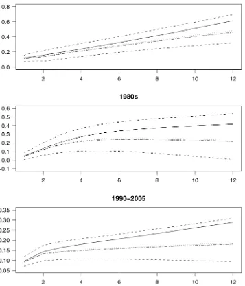
We now turn to the main subject of interest, the estimates of impulse responses. Figure 1 plots the point estimates and the 95% posterior probability bands of responses of CPI (measured in percentage per annum) to a unit shock in PPI of crude materi-als. We also plug in MLE of(,)into the impulse responses; they turn out to be similar to the posterior mean of impulse re-sponses. We compare both of these quantities with the intrinsic Bayesian estimates of impulse responses.
The dynamics of the CPI responses in the pre- and post-1980 samples are distinctly different. For the pre-1980 sample, CPI picks up pace after a unit shock of crude material PPI and keeps rising. For the post-1980 sample, the impulse response of CPI levels off after the shock to PPI of crude materials. The change in the dynamics of impulse responses suggests a structural dif-ference between the pre- and post-1980 samples. For each sub-sample period, the entropy-loss-based Bayesian estimates of impulse responses (the solid lines) are larger in magnitude than the posterior mean estimates (the dotted lines). This is not sur-prising, given the results in Section 2 that the Bayesian estimate
Eis larger than the posterior mean ofand thatEis likely to be larger than the posterior mean of. The difference in the competing estimates of VAR parameters corresponds to a visible difference in point estimates of impulse responses (al-though the posterior mean of the impulse responses is unequal to the impulse response functions of the posterior mean). For the longer forecasting horizon of the impulse response, the dif-ference between the posterior mean and the intrinsic estimator is more profound. With a relatively small sample size and dif-fuse priors, the posterior coverage of the data-generating para-meter can be poor; hence being on the tail of the posterior does not imply that the intrinsic estimator is further from the data-generating parameter than the posterior mean is.
Note that under the intrinsic loss, unit shocks in PPI of crude materials were 2.8% for the 1970s, 1.3% for the 1980s, and 4.1% for the post-1990s. However, for each unit shock in PPI of crude materials, the difference in the estimates of impulse re-sponses under the intrinsic estimator for the pre- and post-1980 periods was much smaller than the difference in the posterior
Figure 1. Estimates of Impulse Responses of Application 1: Response of CPI to PPI Raw Material Shocks. (——, Bayesian estimates of impulse
responses under the entropy loss;· · · ·, posterior mean of impulse responses;− · − · −, plugging MLE into functions of impulse response;− − −−,
95% posterior probability bands.)
mean. In other words, the intrinsic Bayesian estimates suggest that the force of pass-through from PPI to CPI is much more persistent than that indicated by the posterior mean estimator.
5.2 Application 2: A VAR of U.S. Macroeconomic Variables
Bayesian VAR models have been commonly used for analyz-ing multivariate time series macroeconomic data and address-ing policy questions. However, not much attention has been given to the sensitivity of results to researchers’ choice of es-timator. Here we compare various Bayesian estimates of a VAR using quarterly data of the U.S. economy. The variables are real GDP growth, government expenditure growth, growth of real consumer expenditure on nondurables, CPI inflation, growth of M2 money stock, and the Federal Funds Rates (FFRs). The data series are obtained from the FRED database at the Fed-eral Reserve Bank of St Louis. These variables have appeared
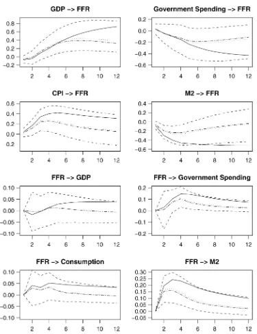
in macroeconomics-related VARs (e.g., Sims 1992; Gordon and Leeper 1994; Sims and Zha 1998; Christiano, Eichenbaum, and Evans 1999). The sample period is 1982Q4–2005Q1, during which the Federal Reserve Bank has been using the FFRs as the main target of monetary policy. The question of interest to us is how the FFRs respond to shocks in macrovariables and how macrovariables respond to shocks in the FFRs. Based on the Bayes information criterion, the lag length of the VAR is set at two.
Table 2 reports the posterior average losses. As is expected, the intrinsic Bayesian estimator produces smaller posterior en-tropy loss than the posterior mean. The latter does better un-der the lossLE1+L2. The impulse responses in Figure 2 show that FFR rises persistently after a shock in GDP growth, based more on the intrinsic Bayesian estimator than on the posterior mean. There is a hump-shaped response of FFR to a shock in CPI inflation. The FFR response to consumption growth shock is close to zero and is not plotted. The slightly positive response
Table 2. Posterior Average Loss in Application 2: 1983.Q1–2005.Q1
LE1 LE2 LE L2 LE1+L2
Mean,Mean 13.214 18,254.000 18,267.214 87.322 100.536
(.072) (240,313.650) (240,313.654) (.552) (.577)
E,E 25.431 69.229 94.660 119.859 145.290
(4.299) (7.945) (12.169) (26.018) (30.113)
NOTE: The subscript “Mean” represents posterior mean estimator, and “E” represents Bayesian estimator under the entropy loss. The lossesLE1andLE2are as given in (9). The entropy loss isLE=LE1+LE2. The quadratic lossL2is as given in (18). The intrinsic Bayesian estimator is optimal under the entropy loss, and the posterior mean estimator is optimal under the lossLE1+L2. Posterior average loss is computed for each MCMC simulation (each with 10,000 cycles after 1,000 burn-in runs). We conducted 1,000 replications of the simulations and report the mean of the posterior average loss (with standard deviations in parentheses) of these replications.
Figure 2. Estimates of Impulse Responses of Application 2: VAR of U.S. Macroeconomic Variables. (——, Bayesian estimates of impulse
responses under the entropy loss;· · · ·, posterior mean of impulse responses;− · − · −, plugging MLE into functions of impulse response;− − −−,
95% posterior probability bands.)
of FFR to M2 money stock growth suggests an absence of liq-uidity effect under the posterior mean; however, the intrinsic Bayesian estimates of FFR response to M2 shocks are larger than the posterior means and exhibit liquidity effect. The re-sponses of macrovariables to shocks in FFR suggest that the latter are not a good indicator of monetary contractions. Both GDP and consumption growth respond positively. Inflation re-sponse to FFR shocks is small and is not plotted. The impulse responses are consistent with the interpretation that shocks in FFR reflect Federal Reserve’s expectation rather than exoge-nous monetary contraction, an interpretation in agreement with the argument of Gordon and Leeper (1994). The intrinsic es-timates offer stronger support to this view than the posterior mean estimates do. The results suggest that more sophisticated characterization of monetary policy is needed. The objective here is to show that the intrinsic Bayesian estimator leads to different estimates than the posterior mean. We leave the task of developing models for monetary policy analysis to future re-search.
6. CONCLUDING REMARKS
In this article we have investigated properties of the Bayesian estimates of impulse responses through an information-theo-retic approach. We have derived Bayesian estimators from an intrinsic entropy loss function and showed that they are dis-tinctly different from the posterior mean. We proposed an algo-rithm that uses generated data as latent variables in numerical simulation of Bayesian estimates under the entropy loss. Our data-augmented simulation scheme may be useful for Bayesian analysis in other problems. For example, in the Bayesian VAR literature, the priors onandare often elicited separately. In this article we examine the Bayesian estimate under the joint nonseparable loss on(,)under separate priors. For users of Bayesian VAR, it is of interest to experiment with joint non-informative priors for(,)under the general principles out-lined by Kass and Wasserman (1996). The joint noninformative priors generally involve frequentist moments of VAR variables, where computational issues similar to our study in the article will arise.
Our work can be extended in a number of ways. First, in this article we consider only estimators of impulse responses under the intrinsic loss. In some VAR applications, researchers may be interested in estimating nonlinear quantities other than im-pulse responses, such as variance decomposition. As noted in Section 1, under the intrinsic loss, any nonlinear quantities can be estimated using the invariance property of the Bayesian esti-mator. We do not pursue this subject in detail, because of space constraints. Second, the present study is limited to estimation of unrestricted VARs. Some recent examples of Bayesian analy-sis with restrictions on parameters in simultaneous equation models and VARs with cointegration include work by Zellner (1998), Gao and Lahiri (2002), Kleibergen and van Dijk (1998), and Kleibergen and Paap (2002). In identified VARs, restric-tions are placed on the contemporaneous relarestric-tionship of VAR variables (e.g., Sims and Zha 1998, 1999). Furthermore, macro-economic theories, such as dynamic stochastic general equilib-rium (DSGE) models, are used for prior elicitation of Bayesian VARs (e.g., Ingram and Whiteman 1994; DeJong et al. 2000;
Del Negro and Schorfheide 2004). Suppose that a DSGE model has fundamental parameterθ (on, e.g., preference, technology, government policies) and that its linearized approximation is a VAR model,
y′t=y′t−1B+ǫ′t, (29) whereǫt∼N(0,). Denote the VAR parametersϒ=(B,). The economic theory corresponds to nonlinear restrictions on ϒ through restrictions ofθ. These theoretical restrictions can be reflected in the prior onϒ. In general, there may be un-observable variables in the DSGE model. In such a case, the DSGE model may be approximated by a state-space model in which Kalman’s filter can be used for evaluating the likelihood. A common practice is to estimate the parameter θ based on a distance between moments of generated data and observed data, for instance, the (IRF) of restricted and unrestricted VARs. This practice does not take into account the uncertainty in the quanti-ties used for estimation, such as the uncertainty in IRF of either restricted or unrestricted VARs. In a Bayesian analysis, such uncertainties are taken into full consideration. Given the eco-nomic theory–based prior and observed data, we can produce Bayesian estimates ofϒunder a loss function. The loss func-tion may be with respect to ϒ or to the IRF of VAR in (29). These estimates imply different estimates forθ. A virtue of the entropy loss is the estimating any nonlinear functions ofϒ, in-cluding the IRF of (29), is equivalent to estimatingθ. Deriving the functional form of the estimator will be difficult, because the likelihood is no longer a standard distribution. Numerical solutions are needed to minimizate the loss function. Bayesian estimation based on intrinsic losses in these settings is chal-lenging and will be left for future research.
ACKNOWLEDGMENTS
The authors thank the editor, an associate editor, and two ref-erees for insightful comments and suggestions that substantially improved the article. Ni’s research was supported by grants from the MU Research Board, MU Research Council, and Hong Kong Research Grant Council (grant CUHK4128/03H). D. Sun’s research was supported by grants from the National Science Foundation (DMS-99-72598 and SES-0351523), the MU Research Board, and the Missouri Department of Conser-vation. The authors benefited from discussions with Christo-pher Sims and Edward George.
APPENDIX A: PROOF OF THEOREM 2
Here we let C,C1,C2, . . . be constants depending only on sample sizeT and observationYD. By Fact 2, withJ=(LP+ 1)p,
RJ
L(φ,)πN(φ)dφ
=C||T/2|M−01+−1⊗(X′DXD)|−1/2
×etr
−1 2
−1S(MLE)
,
where MLE and S(·) are defined by (4) and (5). Because whereŴp(a)is a multivariate gamma function.
APPENDIX B: PROOF OF THEOREM 3
We first state, then prove, a lemma.
Lemma B.1. Suppose that the conditional posterior of φ
given(;YD)is NJ(µ(;YD),V(;YD)). Suppose that for any ,µ(;YD) ≤a0 andV(;YD) <A0, where a0 is a positive constant andA0is a positive definiteJ×Jmatrix, both dependent on data but independent of. Then for any fixed in-tegerk≥0, there exists a constantH(k) >0, that is independent ofsuch that posterior momentE(φk)≤H(k).
Proof. We just need to consider the case k>0, because E(φk)=1 for k=0. Let µ(;YD)=(µ1(;YD), . . . , µJ(;YD))′ and V(;YD) = (σij(;YD))J×J. Then by
µ(;YD) ≤a0 and V(;YD) <A0, we can easily show that there exists a constantC, such that
|µi(;YD)| ≤C, 1≤i≤J, and
Because the posterior is proper from the assumptions, it is sufficient to show that data but is independent of. It follows from Lemma B.1 that for any given integerk≥0, there is a positive constantC1such that
RJ
φkπ(φ|,YD)dφ<C1.
The marginal posterior ofgivenYDhas the form
m(|YD)=C2πb()
Therefore, the left side of (B.1) is bounded by
C4 of Muirhead (1982), (B.2) becomes
C4 because the integrated function in (B.2) is just a function ofλ, whereλ=(λ1, . . . , λp). Note that{pi=1λ2i}h/2≤(pλ1)h and
i . Therefore, (B.3) is bounded by
C5
APPENDIX C: PROOF OF THEOREM 4
By (12) and (13), (E,E) exists if and only if all of plify notation, * that signifies simulated that data are omitted here.
wheregi(φ)is ap-dimensional row vector and each element of gi(φ)is a polynomial of the elements ofφwith degree less than
i+1, Rij(φ)is a p×pmatrix, and each element ofRij(φ)is
a polynomial of the elements ofφ with degree less thani. In Theorem 3 ensures that (C.1) and (C.2) hold under the condition T>2p−b+2. Similarly, we can show that
E(G|YD) <∞ and E(′G|YD) <∞ (C.3) ifT>2p−b+2, and thus the result follows.
[Received November 2004. Revised March 2006.]
REFERENCES
Anderson, T. W. (1984),An Introduction to Multivariate Statistical Analysis
(2nd ed.), New York: Wiley.
Bernardo, J. M., and Juárez, M. A. (2003), “Intrinsic Estimation”, inBayesian
Statistics7, eds. J. M. Bernardo, M. J. Bayarri, J. O. Berger, A. P. Dawid, D. Heckerman, A. F. M. Smith, and M. West, Oxford U.K.: Oxford Univer-sity Press, pp. 465–476.
Blomberg, B. S., and Harris, E. S. (1995), “The Commodity-Consumer Price
Connection: Fact or Fable?”Federal Reserve Bank of San Francisco
Eco-nomic Policy Review, October, 21–38.
Chib, S., and Greenberg, E. (1996), “Markov Chain Monte Carlo Simulation
Methods in Econometrics,”Econometric Theory, 12, 327–335.
Christiano, L. J., Eichenbaum, M., and Evans, C. (1999), “Monetary Policy
Shocks: What Have We Learned and to What End?” inHandbook of
Macro-economics, Vol. 1, eds. J. B. Taylor and M. Woodford, Amsterdam: North-Holland, pp. 65–147.
Clark, T. E. (1995), “Do Producer Prices Lead Consumer Prices?”Federal
Re-serve Bank of Kansas City Economic Review, Third Quarter, 25–39. DeJong, D. N., Ingram, B. F., and Whiteman, C. H. (2000), “A Bayesian
Approach to Dynamic Macroeconomics,” Journal of Econometrics, 98,
203–223.
Del Negro, M., and Schorfheide, F. (2004), “Priors From General Equilibrium
Models for VARs,”International Economic Review, 45, 643–673.
Elerian, O., Chib, S., and Shephard, N. (2001), “Likelihood Inference for
Dis-cretely Observed Nonlinear Diffusions,”Econometrica, 69, 959–993.
Fernandez-Villaverde, J., and Rubio-Ramirez, J. F. (2004), “Comparing
Dy-namic Equilibrium Economies to Data,” Journal of Econometrics, 123,
153–187.
Furlong, F., and Ingenito, R. (1996), “Commodity Prices and Inflation,”Federal
Reserve Bank of San Francisco Economic Review, 2, 27–47.
Gao, C., and Lahiri, K. (2002), “A Comparison of Some Recent Bayesian and Classical Procedures for Simultaneous Equation Models With Weak Instru-ments,” working paper, State University of New York at Albany, Dept. of Economics.
Geisser, S. (1965), “Bayesian Estimation in Multivariate Analysis,”The Annals
of Mathematical Statistics, 36, 150–159.
Gelfand, A. E., and Smith, A. F. M. (1990), “Sampling-Based Approaches to
Calculating Marginal Densities,”Journal of the American Statistical
Associ-ation, 85, 398–409.
Geweke, J. (1989), “Bayesian Inference in Econometric Models Using Monte
Carlo Integration,”Econometrica, 57, 1317–1339.
Gordon, D. B., and Leeper, E. M. (1994), “The Dynamic Impacts of Monetary
Policy: An Exercise in Tentative Identification,”Journal of Political
Econ-omy, 102, 1228–1247.
Ingram, B. F., and Whiteman, C. H. (1994), “Supplementing the Minnesota Prior-Forecasting Macroeconomic Time Series Using Real Business Cycle
Model Priors,”Journal of Monetary Economics, 34, 497–510.
Jeffreys, H. (1961),Probability Theory, New York: Oxford University Press.
Kass, R. E., and Wasserman, L. (1996), “The Selection of Prior
Distribu-tions by Formal Rules,”Journal of the American Statistical Association, 91,
1343–1370.
Kadiyala, K. R., and Karlsson, S. (1997), “Numerical Methods for Estimation
and Inference in Bayesian VAR Models,”Journal of Applied Econometrics,
12, 99–132.
Kilian, L. (1999), “Finite-Sample Properties of Percentile and Percentile-t
Bootstrap Confidence Intervals for Impulse Responses,” Review of
Eco-nomics and Statistics, 81, 652–660.
Kitamura, Y., and Stutzer, M. (1997), “An Information-Theoretic Alternative to
Generalized Method-of-Moments Estimation,”Econometrica, 65, 861–874.
Kleibergen, F., and Paap, R. (2002), “Priors, Posteriors, and Bayes Factors
for a Bayesian Analysis of Cointegration,”Journal of Econometrics, 111,
223–249.
Kleibergen, F., and van Dijk, H. K. (1998), “Bayesian Simultaneous
Equa-tions Analysis Using Reduced-Rank Structures,”Econometric Theory, 14,
701–743.
Koop, G., Pesaran, H., and Potter, S. (1996), “Impulse Response Analysis in
Nonlinear Multivariate Models,”Journal of Econometrics, 74, 119–147.
MacKinnon, J. G., and Smith, A. A., Jr. (1998), “Approximate Bias Correction
in Econometrics,”Journal of Econometrics, 85, 205–230.
Muirhead, R. (1982),Aspects of Multivariate Statistical Theory, New York:
Wiley.
Ni, S., and Sun, D. (2003), “Noninformative Priors and Frequentist Risks of
Bayesian Estimators of Vector-Autoregressive Models,”Journal of
Econo-metrics, 115, 159–197.
Otrok, C., and Whiteman, C. H. (1998), “Bayesian Leading Indicators:
Measur-ing and PredicatMeasur-ing Economic Conditions in Iowa,”International Economic
Review, 39, 997–1014.
Pesaran, H., and Shin, Y. (1998), “Generalized Impulse Response Analysis in
Linear Multivariate Models,”Economics Letters, 58, 17–29.
Press, J. S. (1982),Applied Multivariate Analysis: Using Bayesian and
Fre-quentist Methods of Inference(2nd ed.), FL: Krieger.
Robert, C. P. (1994),The Bayesian Choice, New York: Springer-Verlag.
(1996), “Intrinsic Losses,”Theory and Decision, 40, 191–204.
Robertson, J. C., Tallman, E. W., and Whiteman, C. H. (2005), “Forecasting
Us-ing Relative Entropy,”Journal of Money, Credit, and Banking, 37, 383–402.
Sims, C. A. (1980), “Macroeconomics and Reality,”Econometrica, 48, 1–48.
(1992), “Interpreting the Macroeconomic Time Series Facts: The
Ef-fects of Monetary Policy,”European Economic Review, 38, 975–1000.
Sims, C. A., and Zha, T. (1998), “Does Monetary Policy Generate Recessions?” Working Paper 98-12, Federal Reserve Bank of Atlanta.
(1999), “Error Bands for Impulse Responses,” Econometrica, 67,
1113–1155.
Sun, D., and Ni, S. (2004), “Bayesian Analysis of Vector-Autoregressive
Mod-els With Noninformative Priors,”Journal of Statistical Planning and
Infer-ence, 121, 291–309.
Tanner, M., and Wang, W. H. (1987), “The Calculation of Posterior
Distribu-tions by Data Augmentation,”Journal of the American Statistical
Associa-tion, 82, 528–540.
Tiao, G. C., and Zellner, A. (1964), “On the Bayesian Estimation Analysis of
Multivariate Regression,”Journal of the Royal Statistical Society, Ser. B, 26,
389–399.
Weinhagen, J. (2002), “An Empirical Analysis of Price Transmission by Stage
of Process,”Monthly Labor Review, November, 3–11.
Zellner, A. (1971),An Introduction to Bayesian Inference in Econometrics,
New York: Wiley.
(1978), “Estimation of Functions of Population Means and Regression Coefficients Including Structural Coefficients: A Minimum Expected Loss
Approach,”Journal of Econometrics, 8, 127–158.
(1997), “Maximal Data Information Prior Distributions,” inBayesian
Analysis in Econometrics and Statistics, Lyme, U.K.: Edward Elgar, Chap. 8. (1998), “The Finite-Sample Properties of Simultaneous Equations
Es-timates and Estimators: Bayesian and Non-Bayesian Approaches,”Journal
of Econometrics, 83, 185–212.