Full Terms & Conditions of access and use can be found at
http://www.tandfonline.com/action/journalInformation?journalCode=ubes20
Download by: [Universitas Maritim Raja Ali Haji], [UNIVERSITAS MARITIM RAJA ALI HAJI
TANJUNGPINANG, KEPULAUAN RIAU] Date: 11 January 2016, At: 20:34
Journal of Business & Economic Statistics
ISSN: 0735-0015 (Print) 1537-2707 (Online) Journal homepage: http://www.tandfonline.com/loi/ubes20
Conditional Correlation Models of Autoregressive
Conditional Heteroscedasticity With Nonstationary
GARCH Equations
Cristina Amado & Timo Teräsvirta
To cite this article: Cristina Amado & Timo Teräsvirta (2014) Conditional Correlation Models of Autoregressive Conditional Heteroscedasticity With Nonstationary GARCH Equations, Journal of Business & Economic Statistics, 32:1, 69-87, DOI: 10.1080/07350015.2013.847376
To link to this article: http://dx.doi.org/10.1080/07350015.2013.847376
Accepted author version posted online: 16 Oct 2013.
Submit your article to this journal
Article views: 405
View related articles
Conditional Correlation Models of
Autoregressive Conditional Heteroscedasticity
With Nonstationary GARCH Equations
Cristina A
MADOCREATES, Department of Economics and Business, Aarhus University, DK-8210 Aarhus, Denmark
and N ´ucleo de Investigac¸ ˜ao em Pol´ıticas Econ ´omicas (NIPE), Universidade do Minho, 4710-057 Braga, Portugal ([email protected])
Timo T
ERASVIRTA¨
CREATES, Department of Economics and Business, Aarhus University, DK-8210 Aarhus, Denmark ([email protected])
In this article, we investigate the effects of careful modeling the long-run dynamics of the volatilities of stock market returns on the conditional correlation structure. To this end, we allow the individual un-conditional variances in un-conditional correlation generalized autoregressive un-conditional heteroscedasticity (CC-GARCH) models to change smoothly over time by incorporating a nonstationary component in the variance equations such as the spline-GARCH model and the time-varying (TV)-GARCH model. The variance equations combine the long-run and the short-run dynamic behavior of the volatilities. The struc-ture of the conditional correlation matrix is assumed to be either time independent or to vary over time. We apply our model to pairs of seven daily stock returns belonging to the S&P 500 composite index and traded at the New York Stock Exchange. The results suggest that accounting for deterministic changes in the unconditional variances improves the fit of the multivariate CC-GARCH models to the data. The effect of careful specification of the variance equations on the estimated correlations is variable: in some cases rather small, in others more discernible. We also show empirically that the CC-GARCH models with time-varying unconditional variances using the TV-GARCH model outperform the other models under study in terms of out-of-sample forecasting performance. In addition, we find that portfolio volatility-timing strategies based on time-varying unconditional variances often outperform the unmodeled long-run variances strategy out-of-sample. As a by-product, we generalize news impact surfaces to the situation in which both the GARCH equations and the conditional correlations contain a deterministic component that is a function of time.
KEY WORDS: Forecasting; Multivariate GARCH model; Nonlinear time series; Portfolio allocation; Time-varying unconditional variance.
1. INTRODUCTION
Many financial issues, such as hedging and risk manage-ment, portfolio selection, and asset allocation rely on informa-tion about the covariances or correlainforma-tions between the underly-ing returns. This has motivated the modelunderly-ing of volatility usunderly-ing multivariate financial time series rather than modeling individ-ual returns separately. A number of multivariate generalized autoregressive conditional heteroscedasticity (GARCH) models have been proposed, and some of them have become standard tools for financial analysts. For recent surveys of multivariate GARCH models see Bauwens, Laurent, and Rombouts (2006) and Silvennoinen and Ter¨asvirta (2009).
In the univariate setting, volatility models have been exten-sively investigated. Many modeling proposals of univariate fi-nancial returns have suggested that nonstationarities in return series may be the cause of the extreme persistence of shocks in estimated GARCH models. In particular, Mikosch and St˘aric˘a (2004) showed how the long-range dependence and the “inte-grated GARCH effect” can be explained by unaccounted struc-tural breaks in the unconditional variance. Previously, Diebold (1986) and Lamoureux and Lastrapes (1990) argued that spu-rious long memory may be detected from a time series with structural breaks.
The problem of structural breaks in the conditional variance can be dealt with by assuming that the ARCH or GARCH model is piecewise stationary and detecting the breaks; see, for exam-ple, Berkes et al. (2004), or Lavielle and Teyssi`ere (2006) for the multivariate case. It is also possible to assume, as Dahlhaus and Subba Rao (2006) recently did, that the parameters of the model change smoothly over time such that the conditional variance is locally but not globally stationary. These authors proposed a locally time-varying ARCH process for modeling the nonsta-tionarity in variance. van Bellegem and von Sachs (2004), Engle and Rangel (2008), and, independently, Amado and Ter¨asvirta (2008) (for later versions, see Amado and Ter¨asvirta2012,2013) assumed global nonstationarity and, among other things, devel-oped an approach in which volatility is modeled by a multi-plicative decomposition of the variance to a nonstationary and stationary component. The stationary component is modeled as a GARCH process, whereas the nonstationary one is a determin-istic time-varying component. In van Bellegem and von Sachs
© 2014American Statistical Association Journal of Business & Economic Statistics
January 2014, Vol. 32, No. 1
DOI:10.1080/07350015.2013.847376
69
(2004), this component is estimated nonparametrically using kernel estimation, in Engle and Rangel (2008) it is an exponen-tial spline, whereas Mazur and Pipie´n (2012) used the Fourier Flexible Form of Gallant (1981). Amado and Ter¨asvirta (2012, 2013) described the nonstationary component by a linear combi-nation of logistic functions of time and their generalizations and developed a data-driven specification technique for determining the parametric structure of the time-varying component. The parameters of both the unconditional and the conditional com-ponent were estimated jointly by maximum likelihood (ML). Asymptotic properties of these estimators were considered by Amado and Ter¨asvirta (2013).
Despite the growing literature on multivariate GARCH mod-els, little attention has been devoted to modeling multivariate financial data by explicitly allowing for nonstationarity in vari-ance. Recently, Hafner and Linton (2010) proposed what they called a semiparametric generalization of the scalar multiplica-tive model of Engle and Rangel (2008). Their multivariate GARCH model is a first-order BEKK-GARCH model with a deterministic nonstationary or “long-run” component. In fact, their model is closer in spirit to that of van Bellegem and von Sachs (2004), because they estimated the nonstationary com-ponent nonparametrically. The authors suggested an estimation procedure for the parametric and nonparametric components and established semiparametric efficiency of their estimators.
In this article, we consider a parametric extension of the uni-variate multiplicative GARCH model of Amado and Ter¨asvirta (2012,2013) to the multivariate case. We investigate the effects of careful modeling of the time-varying unconditional variance on the correlation structure of Conditional Correlation GARCH (CC-GARCH) models. To this end, we allow the individual unconditional variances in the multivariate GARCH models to change smoothly over time by incorporating a nonstationary component in the variance equations. The empirical analysis consists of first fitting bivariate CC-GARCH models to pairs of daily return series and comparing the results from models with the time-varying unconditional variance component to models without such a component. Thereafter, we carry out an out-of-sample analysis to evaluate the forecasting performance for the conditional covariances matrices of all individual return series. We also assess the economic value of the time-varying uncon-ditional variance based on CC-GARCH models. For this pur-pose, we implement volatility-timing strategies using both the unmodeled and the modeled time-varying unconditional vari-ance components and evaluate the economic gains in portfolio allocation in the out-of-sample period associated with switch-ing to the model with time-varyswitch-ing unconditional variance. By comparing covariance forecasts in the portfolio selection frame-work, we find that multivariate covariance forecasts based on time-varying unconditional variances are favored over the ones obtained from CC-GARCH models with a constant uncondi-tional variance.
As a by-product, we extend the concept of news impact sur-faces of Kroner and Ng (1998) to the case where both the vari-ances and conditional correlations are fluctuating determinis-tically over time. These surfaces illustrate how the impact of news on covariances between asset returns depends both on the state of the market and the time-varying dependence between the returns.
The article is organized as follows. In Section2, we describe the CC-GARCH model in which the individual unconditional variances change smoothly over time. Estimation of parameters of these models is discussed in Section3 and specification of the unconditional variance components in Section4. Section5 contains the empirical results of fitting bivariate CC-GARCH models to the 21 pairs of seven daily return series of stocks belonging to the S&P 500 composite index and results of an out-of-sample forecasting experiment. Section6comprises an out-of-sample evaluation of the economic value of modeling the time-varying unconditional variances. Generalizations of news impact surfaces are presented in Section7. Conclusions can be found in Section8.
2. THE MODEL
2.1 The General Framework
Consider an N×1 vector of return time series {yt}, t =
1, . . . , T ,described by the following vector process:
yt=E(yt|Ft−1)+εt, (1)
where Ft−1 is the sigma-algebra generated by the avail-able information up until t−1. For simplicity, we assume
E(yt|Ft−1)=0. TheN-dimensional vector of innovations (or now, returns){εt}is defined as
εt =Dtζt, (2)
where Dt is a diagonal matrix of time-varying standard
de-viations. The error vectors ζt form a sequence of indepen-dent and iindepen-dentically distributed variables with mean zero and a positive-definite correlation matrixPt =[ρijt] such thatρiit=1
and|ρijt|<1, i=j, i, j =1, . . . , N.This impliesP−t1/2ζt ∼
iid(0,IN).Under these assumptions, the error vectorεtsatisfies
the following moment conditions:
E(εt|Ft−1)=0
E(εtε′t|Ft−1)=t =DtPtD′t, (3)
where the conditional covariance matrixt =[σijt] ofεt given
the information setFt−1is a positive-definiteN×Nmatrix. It is now assumed thatDtconsists of a conditionally heteroscedastic
component and a deterministic time-dependent one such that
Dt=StGt, (4)
whereSt =diag(h11/t2, . . . , h
1/2
N t) contains the conditional
stan-dard deviations h1it/2, i=1, . . . , N and Gt = diag(g
1/2 1t , . . . ,
g1N t/2).The elementsgit, i =1, . . . , N,are positive-valued de-terministic functions of rescaled time, whose structure will be defined in a moment. Equations (3) and (4) jointly define the time-varying covariance matrix
t =StGtPtGtSt. (5)
It follows that
σijt=ρijt(hitgit)1/2(hjtgjt)1/2, i=j (6)
and that
σiit =hitgit, i=1, . . . , N. (7)
From (7) it follows thathit=σiit/git=E(ε∗itεit∗′|Ft−1),where ε∗it=εit/g
1/2
it . WhenGt ≡IN and the conditional correlation
matrixPt≡P, one obtains the constant conditional correlation
(CCC-)GARCH model of Bollerslev (1990). More generally, whenGt ≡IN andPt is a time-varying correlation matrix, the
model belongs to the family of CC-GARCH models.
Following Amado and Ter¨asvirta (2012,2013), the diagonal elements of the matrixGt are defined as
git=δ0l+
ri
l=1
δilGil(t /T;γil,cil), (8)
where γil>0, i=1, . . . , N, l=1, . . . , ri, and ri =
0,1,2, . . . , R, such that R is a finite integer. The identifica-tion problem arising from the fact that both hit andgit con-tain an intercept is solved by settingδ0l=1.Each git varies smoothly over time satisfying the conditions inft=1,...,T git>0, andδil≤Mδ <∞, l=1, . . . , r,fori=1, . . . , N.For
identi-fication reasons, in (8)δi1<· · ·< δirandδil=0 for alliandl.
The functionGil(t /T;γil,cil) is a generalized logistic function,
that is,
Gil(t /T;γil,cil)=
⎛ ⎝1+exp
⎧ ⎨ ⎩−γil
kil
j=1
(t /T −cilj)
⎫ ⎬ ⎭ ⎞ ⎠
−1
,
γil>0, cil1≤ · · · ≤cilk. (9)
Function (9) is by construction continuous for γil<∞, i =
1, . . . , r,and bounded between zero and one. The parameters ciljandγildetermine the location and the speed of the transition
between regimes.
The parametric form of (8) with (9) is very flexible and ca-pable of describing smooth changes in the amplitude of volatil-ity clusters. Underδi1= · · · =δir=0 orγi1= · · · =γir =0,
i=1, . . . , N,in (8), the unconditional variance ofεtbecomes constant, otherwise it is time-varying. Assuming eitherri >1
orkil>1 or both withδil=0 adds flexibility to the
uncondi-tional variance componentgit.In the simplest case,r=1 and k=1,gitincreases monotonically over time whenδi1>0 and decreases monotonically whenδi1<0.The slope parameterγi1 in (9) controls the degree of smoothness of the transition: the largerγi1,the faster the transition between the extreme regimes. Asγi1→ ∞, git approaches a step function with a switch at ci11. For small values ofγi1,the transition between regimes is very smooth.
In this work, we shall account for potentially asymmetric responses of volatility to positive and negative shocks or returns by assuming the conditional variance components to follow the GJR-GARCH process of Glosten, Jagannathan, and Runkle (1993). In the present context,
hit=ωi+ q
j=1
αijε∗i,t2−j+ q
j=1
κijI(εi,t∗−j <0)ε
∗2
i,t−j
+
p
j=1
βijhi,t−j, (10)
where the indicator functionI(A)=1 whenAis valid, other-wiseI(A)=0.The assumption of a discrete switch atε∗
i,t−j =0
can be generalized following Hagerud (1997), but this extension is left for later work.
2.2 The Structure of the (un)Conditional Correlations
The purpose of this work is to investigate the effects of model-ing changes in the unconditional variances on conditional corre-lation estimates. The idea is to compare the standard approach, in which the nonstationary component is left unmodeled, with the one relying on the decomposition (5) withGt =IN.As to
modeling the time-variation in the correlation matrix Pt,
sev-eral choices exist. As already mentioned, the simplest multivari-ate correlation model is the CCC-GARCH model of Bollerslev (1990) in whichPt ≡P. Withhitspecified as in (10), this model will be called the CCC-TVGJR-GARCH model. Whengit≡1, Equation (10) defines theith conditional variance of the CCC-GJR-GARCH model.
The CCC-GARCH model has considerable appeal due to its computational simplicity, but in many studies the assump-tion of constant correlaassump-tions has been found to be too restric-tive. There are several ways of relaxing this assumption using parametric representations for the correlations. Engle (2002) in-troduced the so-called dynamic CC-GARCH (DCC-GARCH) model in which the conditional correlations are defined through GARCH(1,1) type equations. Tse and Tsui (2002) presented a rather similar model. In the DCC-GARCH model, the coeffi-cient of correlationρijtis a typical element of the matrixPtwith
the dynamic structure
Pt= {diagQt}−1/2Qt{diagQt}−1/2, (11)
where
Qt =(1−θ1−θ2)Q+θ1ζt−1ζ ′
t−1+θ2Qt−1 (12)
such that θ1 >0 and θ2≥0 with θ1+θ2<1, Q is the un-conditional correlation matrix of the standardized errors ζit, i=1, . . . , N,andζt =(ζ1t, . . . , ζN t)′.In our case, eachζit= εit/(hitgit)1/2,and this version of the model will be called the DCC-TVGJR-GARCH model. Accordingly, whengit≡1,the model becomes the DCC-GJR-GARCH model. In the varying correlation (VC-)GARCH model of Tse and Tsui (2002),Pthas
a definition that is slightly different from (12). More specifically,
Pt=(1−θ1−θ2)P+θ1t−1+θ2Pt−1, (13)
where P is a constant positive-definite parameter matrix with unit diagonal elements, θ1 andθ2 are nonnegative parameters such thatθ1+θ2<1,andt−1is the sample correlation matrix of{ζt−1, . . . ,ζt−M}, M ≥N. The positive definiteness ofPtis
ensured ifP0andt−1are positive-definite matrices. In our ap-plication, whenζitis specified asζit=εit/(hitgit)1/2,the model will be called VC-TVGJR-GARCH model. Whengit≡1,the model becomes the VC-GJR-GARCH model.
2.3 Multistep Ahead Forecasting
Constructing one-step-ahead covariance forecasts for the CC-TVGJR-GARCH models discussed in the previous section is straightforward. Since the conditional standard deviations for
the next period are known, we have
Ett+1=St+1|tGt+1|tPt+1|tGt+1|tSt+1|t,
whereSt+1|t is the diagonal matrix holding the one-step-ahead
conditional variance forecasts as described in Section2.1. The low-frequency volatility forecasts included in the matrixGt+1|t
are constructed under the assumption that gi,t+1|t =gi,t, for
all i=1, . . . , N. The d-steps-ahead conditional expectations of the covariance matrix do not have a closed form, and we construct the d-steps-ahead correlation forecasts as in Engle and Sheppard (2001). In the DCC-TVGJR-GARCH model, the correlation forecastPt+1|tis the standardized version ofQt+1|t,
whose one-step-ahead forecast is obtained by projecting (12) one step into the future. In this scheme, the standardized returns areEtζi,t+1=εi,t+1|t/(hi,t+1|tgi,t+1|t)1/2,and
Qt+r|t=(1−θ1−θ2)Q+(θ1+θ2)Qt+r−1|t
for r >1. We construct one-step-ahead forecasts for the VC-TVGJR-GARCH model in an identical fashion.
3. ESTIMATION OF PARAMETERS
The conditional log-likelihood function for observation t of the DCC-TVGJR-GARCH model assuming εt|Ft−1∼
the parameters of the conditional variances, and the el-ements of φ=(θ1, θ2)′ are the parameters of the
cor-Details of estimation of the DCC model can be found in the Appendix.
4. SPECIFYING THE UNCONDITIONAL VARIANCE
COMPONENT
In fitting a model belonging to the family of CC-TVGJR-GARCH models to the data, there are two specification prob-lems. First, one has to determinep andqin (10) andrin (8). Furthermore, ifr≥1,one also has to determinekfor each tran-sition function (9). Second, at least in principle one has to test the null hypothesis of constant conditional correlations against either the DCC- or VC-GARCH model. It appears, however, that in applications involving DCC-GARCH models the null hypothesis of constant conditional correlations is never tested, and we shall adhere to that practice.
We shall thus concentrate on the first set of specification is-sues. We choosep=q=1 and test for higher orders at the evaluation stage. As to selecting r andk, we follow Amado and Ter¨asvirta (2012) and briefly review their procedure. The conditional variances are estimated first, assuming git≡1, i=1, . . . , N.The number of deterministic functionsgitis de-termined thereafter equation by equation by sequential testing. For theith equation, the first hypothesis to be tested is H01: γi1=0 againstH11:γi1>0 in
git=1+δi1Gi1(t /T;γi1,ci1).
The standard test statistic has a nonstandard asymptotic distri-bution becauseδi1 andci1 are unidentified nuisance parame-ters when H01 is true. This lack of identification may be cir-cumvented by following Luukkonen, Saikkonen, and Ter¨asvirta (1988). This means thatGi1(t /T;γi1,ci1) is replaced by its mth-mainder. The new null hypothesis based on this approximation isH′ H01,so the asymptotic distribution theory is not affected by the remainder. As discussed in Amado and Ter¨asvirta (2012), the LM-type test statistic has an asymptotic χ2-distribution with three degrees of freedom whenH01holds.
If the null hypothesis is rejected, the model builder also faces the problem of selecting the order k≤3 in the expo-nent ofGil(t /T;γil,cil). It is solved by carrying out a short
test sequence within (15); for details, see Amado and Ter¨asvirta (2012). The next step is then to estimate the alternative with the chosenk, add another transition, and test the hypothesisγi2=0 in
git=1+δi∗1Gi1(t /T;γi1,ci1)+δi∗2Gi1(t /T;γi2,ci2)
using the same technique as before. Testing continues until the first nonrejection of the null hypothesis. The LM-type test statis-tic still has an asymptostatis-ticχ2-distribution with three degrees of freedom under the null hypothesis.
The model-building cycle for TVGJR-GARCH models for the elements ofDt =StGtof the CC-GARCH model defined by
Equations (3) and (4) consists of specification, estimation, and
2000 2002 2004 2006 2008 -15
-10 -5 0 5 10 15
(a) AXP returns
2000 2002 2004 2006 2008 -15
-10 -5 0 5 10 15
(b) BA returns
2000 2002 2004 2006 2008 -15
-10 -5 0 5 10
(c) CAT returns
2000 2002 2004 2006 2008 -20
-15 -10 -5 0 5 10 15 20
(d) INTC returns
2000 2002 2004 2006 2008 -20
-15 -10 -5 0 5 10 15
(e) JPM returns
2000 2002 2004 2006 2008 -10
-5 0 5 10
(f ) WHR returns
2000 2002 2004 2006 2008 -10
-5 0 5 10
(g) XOM returns
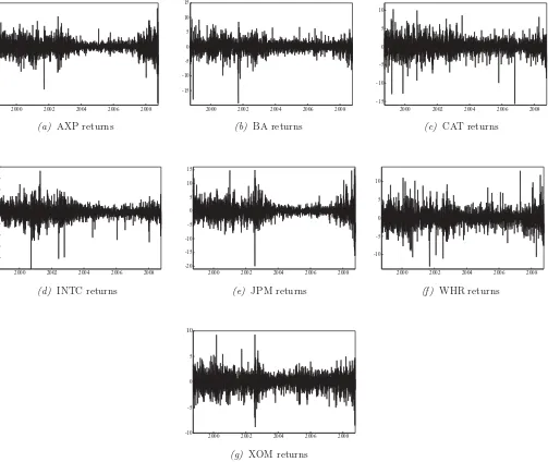
Figure 1. The seven stock returns of the S&P 500 composite index from September 29, 1998, until October 7, 2008 (2521 observations).
evaluation stages. After specifying and estimating the model, the estimated individual TVGJR-GARCH equations will be evalu-ated by means of LM-type diagnostic tests considered in Amado and Ter¨asvirta (2012).
5. EMPIRICAL ANALYSIS I: MODELING AND
FORECASTING
5.1 Data
The effects of careful modeling the nonstationarity in return series on the conditional correlations are studied with price se-ries of seven stocks of the S&P 500 composite index traded at the New York Stock Exchange. The time series are available at the WebsiteYahoo! Finance. They consist of daily closing prices of American Express (AXP), Boeing Company (BA), Caterpillar (CAT), Intel Corporation (INTC), JPMorgan Chase & Co. (JPM), Whirlpool (WHR), and Exxon Mobil Corpora-tion (XOM). The seven companies belong to different industries that are consumer finance (AXP), aerospace and defence (BA),
machines (CAT), semiconductors (INTC), banking (JPM), con-sumption durables (WHR), and energy (XOM). The in-sample observation period begins September 29, 1998, and ends Oc-tober 7, 2008, yielding a total of 2521 observations. All stock prices are converted into continuously compounded rates of re-turn, whose values are plotted inFigure 1. The out-of-sample period extends from October 8, 2008, to December 31, 2009, which amounts to 311 trading days. As will be discussed later, the daily error covariance matrices for this period are constructed from 5-minute returns.
A common pattern is evident in the seven return series. There is a volatile period from the beginning until the middle of the ob-servation period and a less volatile period starting around 2003 that continues almost to the end of the sample. At the very end, it appears that volatility increases again. Moreover, as expected, all series exhibit volatility clustering, but the amplitude of the clusters varies over time.
Descriptive statistics for the individual return series can be found inTable 1. Conventional measures for skewness and kur-tosis and also their robust counterparts are provided for all series.
Table 1. Descriptive statistics of the asset returns
Asset Min Max Mean Std.dev. Skew Ex.Kurt Rob.Sk. Rob.Kr.
AXP −19.35 13.23 0.011 2.280 −0.265 4.864 0.004 0.418
BA −19.39 9.51 0.019 2.069 −0.611 7.215 −0.003 0.106
CAT −15.68 10.32 0.037 2.073 −0.260 3.945 −0.022 0.108
INTC −24.87 18.32 −0.009 2.896 −0.470 6.197 −0.001 0.160
JPM −19.97 15.47 0.025 2.524 0.282 6.901 −0.010 0.396
WHR −13.30 12.95 0.022 2.254 0.183 3.516 0.004 0.272
XOM −8.83 9.29 0.039 1.579 −0.136 2.334 −0.058 0.060
NOTES: The table contains summary statistics for the raw returns of the seven stocks of the S&P 500 composite index. The sample period is from September 29, 1998, until October 7, 2008 (2521 observations). Rob.Sk. denotes the robust measure for skewness based on quantiles proposed by Bowley and the Rob.Kr. is the robust centered coefficient for kurtosis proposed by Moors (see Kim and White2004).
The conventional estimates indicate both nonzero skewness and excess kurtosis: both are typically found in financial asset re-turns. However, conventional measures of skewness and kurto-sis are sensitive to outliers and should therefore be viewed with caution. Kim and White (2004) suggested to look at robust esti-mates of these quantities. The robust measures for skewness are all very close to zero indicating that the return distributions show very little skewness. All robust kurtosis measures are positive, AXP and JPM being extreme examples of this, which suggests excess kurtosis (the robust kurtosis measure equals zero for nor-mally distributed returns) but less than what the conventional measures indicate. The estimates are strictly univariate and any correlations between the series are ignored.
5.2 Modeling the Conditional Variances and Testing for
the Nonstationary Component
We first construct an adequate GJR-GARCH(1,1) model for the conditional variance of each of the seven return series. The estimated models show a distinct IGARCH effect: for the AXP and JPM returns, the estimate ofαi1+κi1/2+βi1even exceeds unity. To save space, the results are not shown here. Results of the constant unconditional variance against a time-varying structure appear inTable 2under the heading “single transition.” The null model is strongly rejected in all seven cases. From the same table it is seen when the single transition model is tested against two transitions (“double transition”) that one transition is enough in all cases. The test sequence for selecting the type of transition shows that not all rejections imply a monotonically increasing functiongit.
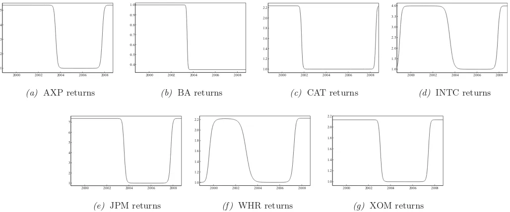
The estimated TVGJR-GARCH models can be found in Tables 3 and 4.Table 4 shows how the persistence measure αi1+κi1/2+βi1 is dramatically smaller in all cases than it is whengit≡1. In two occasions, remarkably low values, 0.782 for CAT and 0.888 for WHR, are obtained. For the remaining se-ries, the reduction in persistence is smaller but still distinct. From Table 3, it can be seen thatgitchanges monotonically only for BA, whereas for the other series this component first decreases and then increases again. In INTC and WHR, however, there is an increase very early on, after which the pattern is similar to that of the other four series. This is also clear fromFigure 2that contains the graphs ofgitfor the seven estimated models.
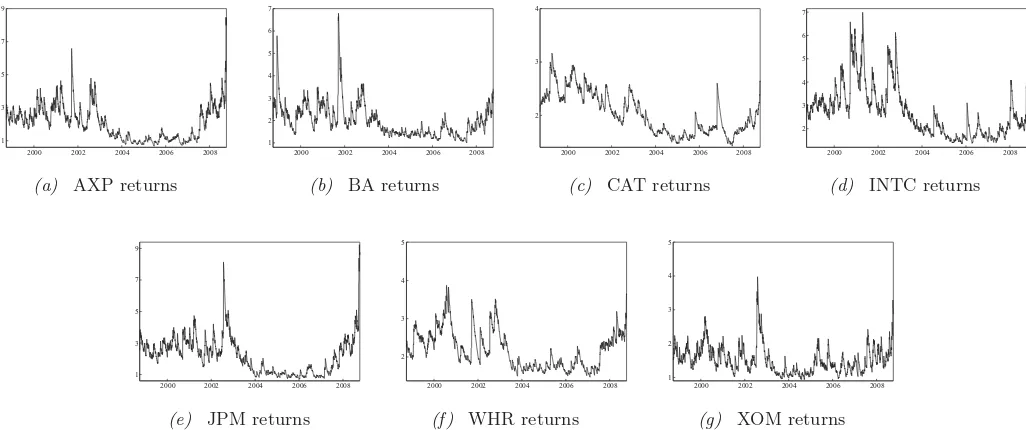
Figures3and4also illustrate the effects of explicitly model-ing the nonstationarity in variance.Figure 3shows the estimated conditional standard deviations from the GJR-GARCH models.
Table 2. Sequence of tests of the GJR-GARCH model against a TVGJR-GARCH model
Transitions H0 H03 H02 H01
Single transition
AXP 0.0184 0.1177 0.0071 0.5722
BA 0.0021 0.0616 0.0461 0.0072
CAT 0.0044 0.0260 0.0107 0.1971
INTC 5×10⁻⁵ 9×10⁻⁵ 0.1600 0.0197
JPM 9×10⁻⁴ 0.0073 0.0023 0.8500
WHR 6×10⁻⁵ 7×10⁻⁴ 0.0011 0.9401
XOM 0.0018 0.0836 7×10⁻⁴ 0.4271
Double transition
AXP 0.0826 0.1953 0.0378 0.4032
BA 0.1208 0.1480 0.0547 0.8419
CAT 0.4011 0.1719 0.4961 0.4347
INTC 0.4307 0.8757 0.1050 0.7458
JPM 0.0947 0.0144 0.8678 0.5484
WHR 0.3059 0.8856 0.1450 0.2249
XOM 0.1111 0.1526 0.4198 0.0685
NOTES: The entries are thep-values of the LM-type tests of constant unconditional variance applied to the seven stock returns of the S&P 500 composite index. The appropriate order kin (9) is chosen from the short sequence of hypothesis as follows: if the smallestp-value of the test corresponds toH02, then choosek=2. If eitherH01orH03are rejected more
strongly thanH02, then select eitherk=1 ork=3. See Amado and Ter¨asvirta (2012) for
further details.
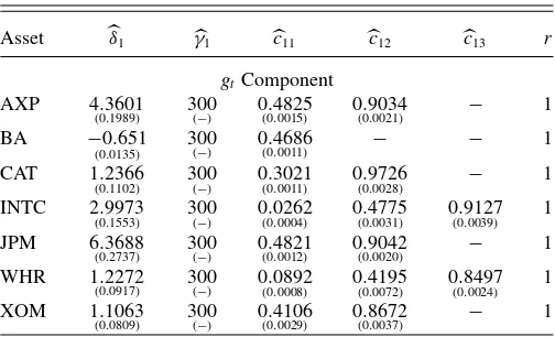
Table 3. Estimation results for the univariate TVGJR-GARCH models
Asset δ1 γ1 c11 c12 c13 r
gt Component
AXP 4.3601
(0.1989) 300(−) 0(0.0015).4825 0(0.0021).9034 − 1
BA −0.651
(0.0135)
300
(−) 0(0.0011).4686 − − 1
CAT 1.2366
(0.1102) 300(−) 0(0.0011).3021 0(0.0028).9726 − 1
INTC 2.9973
(0.1553) 300(−) 0(0.0004).0262 0(0.0031).4775 0(0.0039).9127 1
JPM 6.3688
(0.2737) 300(−) 0(0.0012).4821 0(0.0020).9042 − 1
WHR 1.2272
(0.0917) 300(−) 0(0.0008).0892 0(0.0072).4195 0(0.0024).8497 1
XOM 1.1063
(0.0809) 300(−) 0(0.0029).4106 0(0.0037).8672 − 1
NOTES: The table contains the parameter estimates of thegitcomponent from the
TVGJR-GARCH(1,1) model for the seven stocks of the S&P 500 composite index, over the period September 29, 1998 to October 7, 2008. The estimated model has the formgit=1+
r
l=1δilGil(t /T;γil, cil),whereGil(t /T;δil, cil) is defined in (9) for alli. The numbers in
parentheses are the standard errors.
2000 2002 2004 2006 2008 1
2 3 4 5
(a) AXP returns
2000 2002 2004 2006 2008 0.4
0.5 0.6 0.7 0.8 0.9 1.0
(b) BA returns
2000 2002 2004 2006 2008 1.0
1.2 1.4 1.6 1.8 2.0 2.2
(c) CAT returns
2000 2002 2004 2006 2008 1.0
1.5 2.0 2.5 3.0 3.5 4.0
(d) INTC returns
2000 2002 2004 2006 2008 1
2 3 4 5 6 7
(e) JPM returns
2000 2002 2004 2006 2008 1.0
1.2 1.4 1.6 1.8 2.0 2.2
(f ) WHR returns
2000 2002 2004 2006 2008 1.0
1.2 1.4 1.6 1.8 2.0 2.2
(g) XOM returns
Figure 2. Estimatedgtfunctions for the TVGJR-GARCH model for the seven stock returns of the S&P 500 composite index.
The behavior of these series looks rather nonstationary. The con-ditional standard deviations from the TVGJR-GARCH models can be found inFigure 4. These plots, in contrast to the ones inFigure 3, are rather flat and do not show signs of nonsta-tionarity. The deterministic componentgitis able to absorb the changing “baseline volatility,” and only volatility clustering is left to be parameterized byhit. This is clearly seen from the graphs inFigure 4as they retain the peaks visible inFigure 3. This is what we would expect after the unconditional variance component has absorbed the long-run movements in the series. Results from the spline-GARCH model of Engle and Rangel (2008) are also provided for comparison. The graphs ofgitof the spline-GARCH model for the seven return series are shown inFigure 5. The main differences between the graphs in Figures 2and5appear at their ends, which may have implications for forecasting.Figure 6shows that after the effect of the long-run volatility has been modeled, the conditional standard deviation
Table 4. Estimation results for the univariate TVGJR-GARCH models
Asset ω α1 κ1 β1 α1+κ21+β1
htComponent
AXP 0.0480
(0.0126) 0(0.0114).0045 0(0.0218).1280 0(0.0172).9012 0.9697
BA 0.2994
(0.1448) 0(0.0138).0106 0(0.0353).0851 0(0.0391).9029 0.9561
CAT 0.6641
(0.4611) 0(0.0290).0477 − 0(0.1696).7340 0.7817
INTC 0.1203
(0.0498) 0(0.0165).0450 − 0(0.0269).9155 0.9605
JPM 0.0474
(0.0152) 0(0.0110).0213 0(0.0262).1135 0(0.0229).8890 0.9670
WHR 0.3569
(0.2392) 0(0.0326).0736 − 0(0.1009).8141 0.8877
XOM 0.0644
(0.0222) 0(0.0113).0272 0(0.0215).0578 0(0.0235).9008 0.9568
NOTES: The table contains the parameter estimates of thehitcomponent from the
TVGJR-GARCH(1,1) model for the seven stocks of the S&P 500 composite index, over the period September 29, 1998, to October 7, 2008. The estimated model has the formhit=ωi+
αi1ε∗it2−1+κi1I(ε∗it−1)ε∗it2−1+βi1hit−1,whereε∗it=εit/git1/2andI(εit∗)=1 ifε∗it<0 (and
0 otherwise) for alli. The numbers in parentheses are the Bollerslev–Wooldridge robust standard errors.
series for the standardized returns look stationary as they do in Figure 4. Note that the scales are not comparable, as the ones inFigure 4are based on the assumptionδ0l=1,which is not
a unique solution to the identification problem mentioned in Section2.1.
5.3 Effects of Modeling the Long-Run Dynamics
of Volatility on Correlations
We now study the effects of modeling nonstationary volatil-ity equations on the correlations between pairs of stock returns. Since each individual return series belongs to a different indus-try, we first estimate bivariate CC-GARCH models to investigate the effect on the conditional correlations at the industry level. A bivariate analysis of the returns may also give some idea of how different the correlations between firms representing different industries can be. For that purpose, we consider the CC-GARCH models as defined in Section2.2. For each model, two specifica-tions will be estimated for modeling the univariate volatilities. One is the first-order GJR-GARCH model that corresponds to
Gt ≡I2,whereas the other one is the TVGJR-GARCH model for whichGt =I2in (5).
We begin by comparing the rolling correlation estimates for the (εit, εjt) and (εit/git1/2, εjt/gjt1/2) pairs, wheregjt is given in (8).Figure 7contains the pairwise correlations between the for-mer and the latter computed over 100 trading days. This window size represents a compromise between randomness and smooth-ness in the correlation sequences. The differences are sometimes quite remarkable in the first half of the series where the corre-lations of rescaled returns are often smaller than those of the original returns. In a few cases this is true for the whole se-ries. This might suggest that there are also differences in condi-tional correlations between models based on GJR-GARCH-type variances and their TVGJR-GARCH and spline-GJR-GARCH counterparts. A look atFigure 8suggests, perhaps surprisingly, that when one compares GJR-GARCH models with DCC-TVGJR-GARCH and DCC-Spline-GJR-GARCH ones, this is
2000 2002 2004 2006 2008
2000 2002 2004 2006 2008 1
2000 2002 2004 2006 2008 2
3 4
(c) CAT returns
2000 2002 2004 2006 2008 2
2000 2002 2004 2006 2008 1
2000 2002 2004 2006 2008 2
3 4 5
(f ) WHR returns
2000 2002 2004 2006 2008 1
Figure 3. Estimated conditional standard deviations from the GJR-GARCH(1,1) model for the seven stock returns of the S&P 500 composite index.
2000 2002 2004 2006 2008 1
2000 2002 2004 2006 2008 2
2000 2002 2004 2006 2008 2
3 4
(c) CAT returns
2000 2002 2004 2006 2008 2
2000 2002 2004 2006 2008 1
2000 2002 2004 2006 2008 2
3 4 5
(f ) WHR returns
2000 2002 2004 2006 2008 1
Figure 4. Estimated conditional standard deviations from the GJR-GARCH(1,1) model for the standardized variableεt/gˆ1/2t as in the
TVGJR-GARCH model for the seven stock returns of the S&P 500 composite index.
2000 2002 2004 2006 2008 5
2000 2002 2004 2006 2008 2
2000 2002 2004 2006 2008 3
2000 2002 2004 2006 2008 3
2000 2002 2004 2006 2008 5
2000 2002 2004 2006 2008 4
2000 2002 2004 2006 2008 1.5
Figure 5. Estimatedgtfunctions for the spline-GJR-GARCH model for the seven stock returns of the S&P 500 composite index.
2000 2002 2004 2006 2008 1
3 5 7
(a) AXP returns
2000 2002 2004 2006 2008
1 2 3 4 5
(b) BA returns
2000 2002 2004 2006 2008 1.0
1.5 2.0 2.5 3.0
(c) CAT returns
2000 2002 2004 2006 2008 1.0
1.5 2.0 2.5 3.0 3.5 4.0
(d) INTC returns
2000 2002 2004 2006 2008 2
4 6 8
(e) JPM returns
2000 2002 2004 2006 2008 1.0
1.5 2.0 2.5 3.0 3.5
(f ) WHR returns
2000 2002 2004 2006 2008 1
2 3 4 5
(g) XOM returns
Figure 6. Estimated conditional standard deviations from the GJR-GARCH(1,1) model for the standardized variableεt/gˆ
1/2
t as in the
spline-GJR-GARCH model for the seven stock returns of the S&P 500 composite index.
not the case. The figure depicts the differences between the conditional correlations over time for the 21 bivariate models. They are generally rather small, and it is difficult to find any systematic pattern in them. The CAT-WHR pair is the only ex-ception: the difference between the correlations lies within the interval (−0.22,0.30) in the DCC-TVGJR-GARCH case. The difference in the correlations for the DCC-Spline-GJR-GARCH model is generally larger than that of the DCC-TVGJR-GARCH model. To save space, the correlations estimated from the CCC-and VC-GJR-GARCH models are not shown. A general finding is that the correlations from the CCC-TVGJR-GARCH model remain very close to the ones obtained from the CCC-GJR-GARCH model. The same is true for the VC-TVGJR-CCC-GJR-GARCH model as the modeled nonstationarity in the variances only has a small effect on time-varying correlations. One may thus con-clude that if the focus of the modeler is on conditional correla-tions, taking nonstationarity in the variance into account is not particularly important.
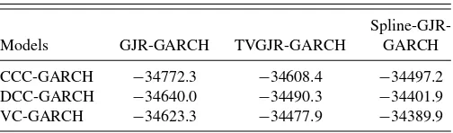
Nevertheless, the fit of the models considerably improves when the unconditional variance component is properly mod-eled. The log-likelihood values for each seven-dimensional CC-GJR-GARCH model are reported inTable 5. The maxima of the log-likelihood functions are substantially higher whengitis esti-mated than when it is ignored. In particular, the best fitting model is the VC-spline-GJR-GARCH model, followed by the DCC-spline-GJR-GARCH and the VC-TVGJR-GARCH model.
Table 5. Log-likelihood values from the seven-variate normal density for the CC-GJR-GARCH models
Spline-GJR-Models GJR-GARCH TVGJR-GARCH GARCH
CCC-GARCH −34772.3 −34608.4 −34497.2
DCC-GARCH −34640.0 −34490.3 −34401.9
VC-GARCH −34623.3 −34477.9 −34389.9
NOTES: The GJR-GARCH column indicates that the unconditional variances are time-invariant functions. The TVGJR-GARCH column indicates that the unconditional variances vary over time according to function (8).
5.4 Evaluating Forecasting Performance
To evaluate the forecasting performance of the multivariate CC-GARCH models, we consider a rolling scheme for the esti-mation of parameters using a fixed window of 2521 daily obser-vations. Specifically, the first set of one-step-ahead covariance forecasts is based on the estimation period from September 29, 1998, until October 7, 2008. To generate the next set of covari-ance forecasts, the window is rolled forward one day to obtain the second set of daily covariance forecasts. We repeat this pro-cess by adding the next observation and discarding the earliest return until we reach the end of the out-of-sample period. After performing this procedure, we compute 311 one-step-ahead co-variance forecasts, each based on the estimation of 2521 returns. As already mentioned, the overall out-of-sample period ranges from October 8, 2008, to December 31, 2009.
The evaluation consists of comparing the predicted covari-ance matrix with the true matrix. Since the true covaricovari-ance ma-trix is unobserved, following Andersen et al. (2003) we use as a proxy the realized covariance estimator defined as the sum of the outer-product of intra-daily returns over the forecast horizon. All computations are based on one-day-ahead forecasts of the covariance matrix over 311 days. The intra-daily data consist of tick-by-tick trade prices for the seven series from the NYSE Trade and Quote database (TAQ) sampled from 9:30 until 16:00 at 5-minute intervals. Intraday returns,rj,t,are computed as
rj,t =pj ,t−p(j−1),t, j =1, . . . , M,
where=1/Mandpj ,tis the log price at timej in dayt.
In Figure 9, we plot the differences between the esti-mated correlations obtained from the seven-dimensional VC-GJR-GARCH and the VC-TVGJR-GARCH models in the out-of-sample period. The differences in correlations between the two DCC-GARCH models are not shown since they do not differ much from those found in-sample. The conditional correlations estimated from the VC-GJR-GARCH model are generally larger than the ones obtained from the VC-TVGJR-GARCH model, but the differences are rather small. With few
2000 2002 2004 2006 2008
2000 2002 2004 2006 2008 0.0
2000 2002 2004 2006 2008 0.0
2000 2002 2004 2006 2008 0.0
2000 2002 2004 2006 2008 -0.2
2000 2002 2004 2006 2008 0.0
2000 2002 2004 2006 2008 0.0
2000 2002 2004 2006 2008 0.0
2000 2002 2004 2006 2008 0.0
2000 2002 2004 2006 2008 0.0
2000 2002 2004 2006 2008 0.0
2000 2002 2004 2006 2008 0.0
2000 2002 2004 2006 2008 0.0
2000 2002 2004 2006 2008 0.0
2000 2002 2004 2006 2008 0.0
2000 2002 2004 2006 2008 -0.2
2000 2002 2004 2006 2008 -0.2
2000 2002 2004 2006 2008 0.0
2000 2002 2004 2006 2008 -0.2
2000 2002 2004 2006 2008 -0.2
2000 2002 2004 2006 2008 0.0
Figure 7. Differences between the estimated rolling correlation coefficients for pairs of the raw returns (gray curve) and pairs of the standardized returns (black curve).
78
2000 2002 2004 2006 2008
2000 2002 2004 2006 2008
-0.05
-0.02
0.01
0.04
(b) AXP-CAT
2000 2002 2004 2006 2008
-0.08
-0.04
0.00
0.04
(c) BA-CAT
2000 2002 2004 2006 2008
-0.06
2000 2002 2004 2006 2008
-0.07
-0.03
0.01
0.05
(e) BA-INTC
2000 2002 2004 2006 2008
-0.04
2000 2002 2004 2006 2008
-0.05
-0.02
0.01
0.04
(g) AXP-JPM
2000 2002 2004 2006 2008
-0.2
-0.1
0.0
0.1
(h)BA-JPM
2000 2002 2004 2006 2008
-0.06
2000 2002 2004 2006 2008
-0.04
2000 2002 2004 2006 2008
-0.16
2000 2002 2004 2006 2008
-0.10
-0.04
0.02
0.08
(l)BA-WHR
2000 2002 2004 2006 2008
-0.2
2000 2002 2004 2006 2008
-0.05
-0.02
0.01
0.04
(n) INTC-WHR
2000 2002 2004 2006 2008
-0.15
-0.05
0.05
0.15
(o) JPM-WHR
2000 2002 2004 2006 2008
-0.06
2000 2002 2004 2006 2008
-0.06
2000 2002 2004 2006 2008
-0.03
-0.01
0.01
0.03
(r) CAT-XOM
2000 2002 2004 2006 2008
-0.06
2000 2002 2004 2006 2008
-0.04
2000 2002 2004 2006 2008
-0.3
-0.1
0.1
0.3
(u) WHR-XOM
Figure 8. Differences between the estimated conditional correlations obtained from the bivariate DCC-GJR-GARCH and the DCC-TVGJR-GARCH models (black curve), and difference between the estimated conditional correlations obtained from the bivariate DCC-GJR-GARCH and the DCC-Spline-GJR-GARCH models (gray curve) for the asset returns.
79
0 50 100 150 200 250 300 0.01
0.03 0.05 0.07
(a) AXP-BA
0 50 100 150 200 250 300 0.01
0.03 0.05 0.07
(b) AXP-CAT
0 50 100 150 200 250 300 0.01
0.03 0.05 0.07
(c) BA-CAT
0 50 100 150 200 250 300 0.01
0.03 0.05 0.07
(d)AXP-INTC
0 50 100 150 200 250 300 0.01
0.03 0.05 0.07
(e) BA-INTC
0 50 100 150 200 250 300 0.01
0.03 0.05 0.07
(f ) CAT-INTC
0 50 100 150 200 250 300 0.01
0.03 0.05 0.07
(g) AXP-JPM
0 50 100 150 200 250 300 0.01
0.03 0.05 0.07
(h) BA-JPM
0 50 100 150 200 250 300 0.01
0.03 0.05 0.07
(i) CAT-JPM
0 50 100 150 200 250 300 0.01
0.03 0.05 0.07
(j) INTC-JPM
0 50 100 150 200 250 300 0.01
0.03 0.05 0.07
(k) AXP-WHR
0 50 100 150 200 250 300 0.01
0.03 0.05 0.07
(l)BA-WHR
0 50 100 150 200 250 300 0.01
0.03 0.05 0.07
(m) CAT-WHR
0 50 100 150 200 250 300 0.01
0.03 0.05 0.07
(n) INTC-WHR
0 50 100 150 200 250 300 0.01
0.03 0.05 0.07
(o) JPM-WHR
0 50 100 150 200 250 300 −0.01
0.01 0.03 0.05 0.07
(p)AXP-XOM
0 50 100 150 200 250 300 0.01
0.03 0.05 0.07
(q) BA-XOM
0 50 100 150 200 250 300 0.01
0.03 0.05 0.07
(r) CAT-XOM
0 50 100 150 200 250 300 0.01
0.03 0.05 0.07
(s)INTC-XOM
0 50 100 150 200 250 300 −0.01
0.01 0.03 0.05 0.07
(t) JPM-XOM
0 50 100 150 200 250 300 −0.3
−0.1 0.1 0.3 0.5 0.7
(u) WHR-XOM
Figure 9. Differences between the estimated conditional correlations obtained from the seven-variate VC-GJR-GARCH and the seven-variate VC-TVGJR-GARCH models for the asset returns in the out-of-sample period from October 8, 2008, to December 31, 2009.
80
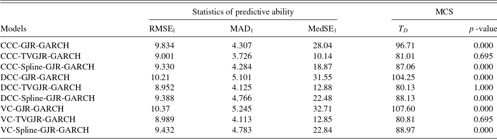
Table 6. Out-of-sample prediction accuracy for the conditional covariance matrices
Statistics of predictive ability MCS
Models RMSE1 MAD1 MedSE1 TD p-value
CCC-GJR-GARCH 9.834 4.307 28.04 96.71 0.000
CCC-TVGJR-GARCH 9.001 3.726 10.14 81.01 0.695
CCC-Spline-GJR-GARCH 9.330 4.284 18.87 87.06 0.000
DCC-GJR-GARCH 10.21 5.101 31.55 104.25 0.000
DCC-TVGJR-GARCH 8.952 4.125 12.88 80.13 1.000
DCC-Spline-GJR-GARCH 9.388 4.766 22.48 88.13 0.000
VC-GJR-GARCH 10.37 5.245 32.71 107.60 0.000
VC-TVGJR-GARCH 8.989 4.113 12.85 80.81 0.695
VC-Spline-GJR-GARCH 9.432 4.783 22.84 88.97 0.000
NOTES: The out-of-sample forecast evaluation statistics are the root mean squared error (RMSE), the mean absolute deviation (MAD), and the median squared error (MedSE) criteria. The loss function is based on the Frobenius distance of the forecast error as in Patton and Sheppard (2009). The test statisticTDdenotes the deviation statistic of Hansen, Lunde, and
Nason (2011). The results are based on the out-of-sample data from October 8, 2008, to December 31, 2009 (311 observations).
exceptions, the difference reaches its maximum around the middle of the period, after which it suddenly decreases.
To compare the accuracy of the one-day-ahead covariance matrix forecasts, we consider the following loss function based on the Frobenius distance of the forecast error; see Patton and Sheppard (2009):
LF,T+i =(1/N2){vec(T+i−T+i)′vec(T+i−T+i)},
where T+i is the one-step-ahead forecast of the covariance
matrix for timeT +i andT+i is the true covariance matrix
proxied by the realized covariance estimator. This function is the squared error generalized to matrix spaces. To measure the fore-casting performance, we shall consider the root mean squared error (RMSE) but also the mean absolute deviation (MAD) based on theL1norm:
L1,T+i=(1/N2){vec(T+i−T+i)1}.
Criteria based on the absolute deviations are sometimes pre-ferred because they are less affected by outliers than RMSE. To reduce the impact of outlying observations on forecasting eval-uation even further, we also report values of the median squared error (MedSE). Note, however, that MAD and MedSE are not consistent criteria in the sense that they do not necessarily pre-serve the correct ordering of the losses from the models under consideration when the true covariance matrix is unknown; see Laurent, Rombouts, and Violante (2013) for discussion.
Table 6presents values of the three criteria for the 1-day horizon. According to MAD and MedSE, the models with time-varying unconditional variances perform better than the ones without this feature. Interestingly, the CCC-TVGJR-GARCH model outperforms the others, which suggests that modeling time variation in correlations is not crucial in forecasting, at least not in the short run. If we instead consider RMSE as a measure of predictive ability, the differences between models are very small, and now the DCC-TVGJR-GARCH model is slightly superior to the rest. Obviously, the CC-TVGJR-GARCH models generate some rather inaccurate forecasts that are downweighted by the use of MAD or MedSE.
In addition, to test joint forecasting performance across all models we make use of the model confidence set (MCS) ap-proach of Hansen, Lunde, and Nason (2011). We set the con-fidence level of MCS equal to 0.1. The block length equals
two, and the number of bootstrap samples is 10,000. The results can be found inTable 6. MCS contains the three CC-TVGJR-GARCH models. This means that out-of-sample performance of the CC-GJR-GARCH models with time-varying uncondi-tional variance is superior to that of the models with constant unconditional variance. It also means that in this experiment the TV-GARCH approach performs somewhat better than the spline-GARCH one. A general conclusion is that careful model-ing of the unconditional variance is very important in forecastmodel-ing covariance matrices, at least in the short run.
6. EMPIRICAL ANALYSIS II: PORTFOLIO
ALLOCATION
Another way of evaluating our models out-of-sample is to consider the economic value of volatility timing; see Fleming, Kirby, and Ostdiek (2001) and Engle and Colacito (2006) among others. We do this by applying three portfolio allocation strate-gies both when the unconditional variance is time-varying and when it is not. These optimal asset-allocation strategies are the global minimum variance (GMV), the minimum variance with target expected return (min-variance), and the mean-variance (mean-variance) strategy. In implementing them, the weights are based on forecasts of the conditional covariance matrix as-sociated with each CC-GARCH model.
According to the mean-variance strategy, for each timetthe investor solves the quadratic programing problem
min wt
w′ttwt−
1 γμ
′
twt s.t. w′t1=1,
where wt is an N×1 vector of portfolio weights, μt is the
N×1 vector of expected returns,1is anN-dimensional vector of ones, andγis the risk aversion parameter. The GMV strategy corresponds to the mean-variance portfolio with an infinite risk aversion parameter. The min-variance strategy aims at finding the portfolio that has the smallest risk, measured by the portfolio variance, which achieves a target expected return
min wt
w′ttwt s.t. w′tμt=μp andw′t1=1,
whereμp is the target expected rate of return of the portfolio.
We set μp=8. No short selling restrictions are imposed on
any strategy.
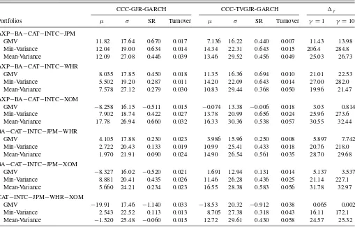
Table 7. Out-of-sample portfolio performance of the volatility-timing strategies: CCC-GJR-GARCH versus CCC-TVGJR-GARCH
CCC-GJR-GARCH CCC-TVGJR-GARCH γ
Portfolios μ σ SR Turnover μ σ SR Turnover γ =1 γ =10
AXP−BA−CAT−INTC−JPM
GMV 11.82 17.64 0.670 0.017 7.136 16.22 0.440 0.007 11.43 13.98
Min-Variance 12.04 19.00 0.634 0.014 14.34 22.31 0.643 0.015 206.4 284.8
Mean-Variance 12.09 27.08 0.446 0.039 13.46 29.52 0.456 0.049 25.03 26.73
AXP−BA−CAT−INTC−WHR
GMV 8.035 17.85 0.450 0.018 11.35 16.36 0.694 0.010 21.01 22.53
Min-Variance 5.502 19.20 0.287 0.011 14.20 22.09 0.643 0.014 27.00 282.0
Mean-Variance 7.578 27.12 0.279 0.030 10.83 29.44 0.368 0.050 19.96 21.47
AXP−BA−CAT−INTC−XOM
GMV −8.258 16.15 −0.511 0.015 −0.074 13.38 −0.006 0.018 3.03 0.814
Min-Variance 7.902 18.74 0.422 0.027 13.78 20.99 0.656 0.024 25.96 273.6
Mean-Variance 17.78 26.94 0.660 0.032 16.33 30.36 0.538 0.057 30.55 32.44
BA−CAT−INTC−JPM−WHR
GMV 4.105 17.88 0.230 0.023 3.986 15.96 0.250 0.008 5.897 7.742
Min-Variance 2.722 20.43 0.133 0.019 10.99 25.41 0.433 0.018 20.76 218.0
Mean-Variance 1.970 21.91 0.090 0.024 14.90 26.54 0.561 0.035 28.70 29.68
BA−CAT−INTC−JPM−XOM
GMV −8.327 16.02 −0.520 0.021 1.691 12.94 0.131 0.014 5.137 3.537
Min-Variance 8.881 20.41 0.435 0.026 11.46 26.28 0.436 0.025 21.14 227.1
Mean-Variance 5.660 24.21 0.234 0.023 16.55 28.38 0.583 0.056 31.78 32.97
CAT−INTC−JPM−WHR−XOM
GMV −19.91 17.46 −1.140 0.033 −18.53 20.32 −0.912 0.038 0.065 0.002
Min-Variance 2.543 22.52 0.113 0.013 8.705 27.38 0.318 0.043 16.11 172.1
Mean-Variance −1.520 25.48 −0.060 0.015 12.72 29.61 0.430 0.058 24.57 25.32
NOTES: The table summarizes the out-of-sample performance for three sets of portfolio dynamic weights: global minimum variance (GMV), minimum variance with target expected return equal to 8% (min-variance) and mean-variance (mean-variance) portfolio strategy. For each set of weights, we report the annualized mean excess returns (μ), the annualized standard deviation (σ), the annualized Sharpe ratio (SR), and the average daily turnover over the out-of-sample period from October 8, 2008, to December 31, 2009. We also report the average annualized basis point fees that an investor with quadratic utility and constant relative risk aversion ofγ=1 orγ=10 would be willing to pay to switch from the constant to the time-varying unconditional variance strategy.
For each strategy, we compute the annualized excess returns, the annualized standard deviation, and the annualized Sharpe ratio (SR). We form six portfolios, each containing five stocks, each representing a different industry. The portfolios are rebal-anced daily for each covariance estimator CC-GARCH model. As the risk-free asset needed for computing SRs, we use the 3 month Treasury bill rate. Following Fleming, Kirby, and Ostdiek (2001), we also consider a utility-based measure denoted byγ
to compare the performance of any CC-TVGJR-GARCH model to that of the corresponding CC-GJR-GARCH model. The value ofγ is such that an investor with a quadratic utility function
and the relative risk aversion parameterγis indifferent between receivingrtandrTVt−γ,wherertis the out-of-sample
port-folio return under the CC-GJR-GARCH model and rTVt the
corresponding return under the CC-TVGJR-GARCH model. Tables7and8report the out-of-sample portfolio performance of the volatility-timing strategies for the CCC-GARCH and the DCC-GARCH models. As an indicator for the transaction costs, we also show the portfolio turnover defined as the average of daily absolute changes in portfolio weights|wit−wit−|over the
period, wherewitis the optimal weight of assetion daytand wit−is the weight of the same asset at the end of the dayt−1,
that is, before rebalancing the portfolio. The results show that when the time-varying unconditional variance is modeled, the annualized standard deviation of the portfolios tends to increase in two cases out of three, the GMV strategy being an
excep-tion. But then, with rather few exceptions, the strategies using covariance matrices with time-varying unconditional variances generate higher SRs than those based on unmodeled long-run variances. This is mainly due to the increase of the annualized excess returns of the investment portfolios. The asset combina-tion BA-CAT-INTC-JPM-XOM is the most notable example of this. A move from the GJR-GARCH model to the DCC-TVGJR-GARCH one pushes the expected excess returns of the mean-variance portfolio up from 2.24% to 21.45%. This in turn translates into an increase of the SR from 0.030 to 0.753. Large differences in the SR in favor of CC-TVGJR-GARCH models can be seen in most occasions. This is true both for the constant and for the dynamic conditional correlation models. Applying VC-GJR-GARCH models leads to similar conclusions, so the results are omitted to save space.
DeMiguel and Nogales (2009) indicated that the mean-variance portfolio usually has more unstable weights than the others. This implies a higher portfolio turnover and higher trans-action costs. Our results accord with this observation. When the unconditional variances are time-varying, the weights of this portfolio strategy tend to fluctuate more over time than when they are not. On the other hand, the turnover rates of the GMV and min-variance strategies tend to be lower when the long-run variances are modeled than when they are not. One can thus argue that the CCC-TVGJR-GARCH and the DCC-TVGJR-GARCH models outperform their conventional
Table 8. Out-of-sample portfolio performance of the volatility-timing strategies: DCC-GJR-GARCH versus DCC-TVGJR-GARCH
DCC-GJR-GARCH DCC-TVGJR-GARCH γ
Portfolios μ σ SR Turnover μ σ SR Turnover γ=1 γ =10
AXP−BA−CAT−INTC−JPM
GMV 10.09 22.81 0.442 0.013 5.325 16.59 0.321 0.007 7.442 10.41
Min-Variance 21.51 27.81 0.773 0.015 13.97 22.78 0.613 0.014 25.79 27.71
Mean-Variance 18.10 25.39 0.713 0.027 14.67 29.23 0.502 0.042 27.11 29.14
AXP−BA−CAT−INTC−WHR
GMV 3.707 18.49 0.200 0.016 3.944 17.08 0.231 0.010 6.000 7.720
Min-Variance 5.435 19.90 0.273 0.011 7.602 22.71 0.335 0.013 13.47 14.98
Mean-Variance 2.881 27.19 0.106 0.030 4.166 29.20 0.143 0.043 6.690 8.142
AXP−BA−CAT−INTC−XOM
GMV −10.57 16.38 −0.645 0.018 −3.164 13.71 −0.231 0.012 1.415 0.070
Min-Variance 7.685 19.13 0.402 0.032 12.67 21.41 0.591 0.022 23.69 25.11
Mean-Variance 17.70 26.98 0.656 0.029 15.06 30.41 0.495 0.049 27.92 29.89
BA−CAT−INTC−JPM−WHR
GMV −0.601 18.18 −0.033 0.024 2.037 16.32 0.125 0.006 3.553 4.000
Min-Variance 4.325 20.98 0.206 0.015 9.648 25.90 0.373 0.017 17.88 19.14
Mean-Variance 2.485 22.11 0.112 0.021 18.30 26.98 0.678 0.054 35.49 36.49
BA−CAT−INTC−JPM−XOM
GMV −9.261 16.09 −0.576 0.022 −1.549 13.25 −0.117 0.009 2.079 0.289
Min-Variance 5.255 20.61 0.255 0.018 9.991 26.50 0.377 0.024 18.48 19.81
Mean-Variance 2.237 23.82 0.094 0.030 21.45 28.49 0.753 0.068 41.82 42.80
CAT−INTC−JPM−WHR−XOM
GMV −17.69 17.79 −0.995 0.026 −30.68 20.67 −1.485 0.039 −0.421 −0.051
Min-Variance 3.927 22.83 0.172 0.015 8.359 27.86 0.300 0.028 15.24 16.52
Mean-Variance 0.439 25.53 0.017 0.034 13.20 30.17 0.438 0.058 25.38 26.28
NOTES: The table summarizes the out-of-sample performance for three sets of portfolio dynamic weights: global minimum variance (GMV), minimum variance with target expected return equal to 8% (min-variance), and mean-variance (mean-variance) portfolio strategy. For each set of weights, we report the annualized mean excess returns (μ), the annualized standard deviation (σ), the annualized Sharpe ratio (SR), and the average daily turnover over the out-of-sample period from October 8, 2008, to December 31, 2009. We also report the average annualized basis point fees that an investor with quadratic utility and constant relative risk aversion ofγ=1 orγ=10 would be willing to pay to switch from the constant to the time-varying unconditional variance strategy.
counterparts when these two portfolio strategies are being applied.
Finally, Tables7 and8 also contain the estimates ofγ as
annualized fees in basis points using two different risk aversion parameters, γ =1 and γ =10. Over all six asset combina-tions and the three strategies, a conservative investor,γ =10, would be willing to pay an annual management fee between the minimum, 0.002 (−0.051) basis points, and maximum, 284.8 (42.80) points, when implementing the CCC-TVGJR-GARCH (DCC-TVGJR-GARCH) method. These outcomes strengthen the impression that the conditional correlation models with time-varying unconditional variances outperform their counterparts with constant unconditional variances.
7. TIME-VARYING NEWS IMPACT SURFACES
In this section, we consider the impact of unexpected shocks to the asset returns on the estimated covariances. This is done by employing a generalization of the univariatenews impact curve of Engle and Ng (1993) to the multivariate case introduced by Kroner and Ng (1998). The so-called news impact surfaceis the plot of the conditional covariance against a pair of lagged shocks, holding the past conditional covariances constant at their unconditional sample mean levels. The news impact surfaces of the multivariate correlation models with the volatility equations modeled as TVGJR-GARCH models are time-varying because
they depend on the componentgi,t−1.They will be called time-varying news impact surfaces. The time-time-varying news impact surface forhijtis the three-dimensional graph of the function
hijt=f
εi,t−1/g 1/2
i,t−1, εj,t−1/g 1/2
j,t−1, ρij,t−1;ht−1
,
whereht−1is a vector of conditional covariances at timet−1 defined at their unconditional sample means. As an example, Figure 10contains the time-varying news impact surface for the covariance generated by the CCC-TVGJR-GARCH model for the pair BA-XOM. The choice of this particular pair of assets is merely illustrative, but similar surfaces can be found for other pairs as well. It is seen how the surface can vary over time due to the nonstationary componentsgi,t−1andgj,t−1.We are able to distinguish different reaction levels of covariance estimates to past shocks during tranquil and turbulent times. It shows that the response to the news of a given size on the estimated covariances is clearly stronger during periods of calm in the market (“lower regime”) than it is during periods of high turbulence. According to the results, when calm prevails a minor piece of “bad news” (unexpected negative shock) is rather big news compared to a big piece of “good news” (unexpected positive shock) during turbulent periods. This is seen from the asymmetric bowl-shaped impact surface.
Figure 11 contains the time-varying news impact surfaces under low and high volatility from the CCC-TVGJR-GARCH
BA
XOM -1
0 1
2
-1 0 1 2
0.055
0.060
0.065
(a) lower regime
BA
XOM -1
0 1
2
-1 0 1 2
0.055
0.060
0.065
(b) upper regime
Figure 10. Estimated time-varying news impact surfaces for the covariance between the BA and XOM returns under the CCC-TVGJR-GARCH model (a) in the lower regime and (b) in the upper regime of volatility.
Variance of BA
BA
XOM -1
0
1
-1 0 1
2.48
2.51
2.54
2.57
(a) lower regime
Variance of BA
BA
XOM -1
0
1
-1 0 1
2.48
2.51
2.54
2.57
(b) upper regime
Figure 11. Estimated time-varying news impact surfaces for the conditional variance of the BA returns under the CCC-TVGJR-GARCH model (a) in the lower regime and (b) in the upper regime of volatility.
Variance of XOM
BA
XOM -1
0 1
2
-1 0 1 2
1.10
1.14
1.18
1.22
(a) lower regime
Variance of XOM
BA
XOM -1
0 1
2
-1 0 1 2
1.10
1.14
1.18
1.22
(b) upper regime
Figure 12. Estimated time-varying news impact surfaces for the conditional variance of the XOM returns under the CCC-TVGJR-GARCH model (a) in the lower regime and (b) in the upper regime of volatility.
model for the conditional variance of BA when there is no shock to XOM.Figure 12contains a similar graph for XOM when there is no shock to BA. The asymmetric shape shows that a negative return shock has a greater impact than a positive return shock of the same size. Furthermore, as already seen fromFigure 10, a piece of news of a given size has a stronger effect on the con-ditional variance when volatility is low than when it is high.
8. CONCLUSIONS
In this article, we extend the univariate multiplicative TV-GARCH model of Amado and Ter¨asvirta (2012,2013) to the multivariate CC-GARCH framework. The model allows the in-dividual variances to vary smoothly over time according to the logistic transition function and its generalizations. We develop a modeling technique for specifying the parametric structure of the deterministic time-varying component that involves a se-quence of LM-type tests. In this respect, our model differs from the semiparametric model of Hafner and Linton (2010).
We consider a set of CC-GARCH models to investigate the effects of nonstationary variance equations on the conditional correlation matrix. The models are applied to pairs of seven daily stock returns belonging to the S&P 500 composite in-dex and to the seven-variate case. We find that modeling the time-variation of the unconditional variances considerably im-proves the fit of the CC-GARCH models. The results show that multivariate correlation models combining both time-varying correlations and time-varying unconditional variances provide the best in-sample fit. They also indicate that modeling the non-stationary component in the variance has relatively little effect on correlation estimates when the conditional correlation model is the DCC-GARCH model.
The results on forecasting show that the CC-GARCH models with time-varying unconditional variances clearly outperform the others when the comparison is made using criteria robust to outliers. An interesting finding is that the CCC-TVGJR-GARCH model performs best, which suggests that modeling time variation in correlations is not crucial in forecasting, at least not in the short run. Moreover, the out-of-sample port-folio analysis indicates that modeling the time-varying uncon-ditional volatility is economically relevant. By applying three asset-allocation strategies, we find that the conditional corre-lation models with time-varying unconditional variances tend to outperform their counterparts with constant unconditional variances.
APPENDIX: MAXIMUM LIKELIHOOD ESTIMATION OF PARAMETERS
Equation (14) implies the following decomposition of the log-likelihood function for observationt:
ℓt(ψ,ϕ,φ)=ℓUt (ψ)+ℓ
As is usual in the case of DCC-GARCH models, estimation is carried out in two steps. The GARCH equations are estimated first using maximization by parts, andφin (A.1) conditionally on GARCH estimates.
Maximization by parts works as follows: First, reparameterize the deterministic component (8) as follows:
git∗=δi∗0+
The second iteration is as follows:
1. Maximize