Full Terms & Conditions of access and use can be found at
http://www.tandfonline.com/action/journalInformation?journalCode=ubes20
Download by: [Universitas Maritim Raja Ali Haji] Date: 12 January 2016, At: 17:28
Journal of Business & Economic Statistics
ISSN: 0735-0015 (Print) 1537-2707 (Online) Journal homepage: http://www.tandfonline.com/loi/ubes20
Testing for Shifts in Trend With an Integrated or
Stationary Noise Component
Pierre Perron & Tomoyoshi Yabu
To cite this article: Pierre Perron & Tomoyoshi Yabu (2009) Testing for Shifts in Trend With an Integrated or Stationary Noise Component, Journal of Business & Economic Statistics, 27:3, 369-396, DOI: 10.1198/jbes.2009.07268
To link to this article: http://dx.doi.org/10.1198/jbes.2009.07268
Published online: 01 Jan 2012.
Submit your article to this journal
Article views: 371
View related articles
Testing for Shifts in Trend With an Integrated or
Stationary Noise Component
Pierre PERRON
Department of Economics, Boston University, Boston, MA 02215 (perron@bu.edu)
Tomoyoshi Y
ABUFaculty of Business and Commerce, Keio University, Tokyo 108-8345, Japan (tyabu@fbc.keio.ac.jp)
We consider testing for structural changes in the trend function of a time series without any prior knowl-edge of whether the noise component is stationary or integrated. Following Perron and Yabu (2009), we consider a quasi-feasible generalized least squares procedure that uses a super-efficient estimate of the sum of the autoregressive parametersαwhenα=1. This allows tests of basically the same size with stationary or integrated noise regardless of whether the break is known or unknown, provided that the Exp functional of Andrews and Ploberger (1994) is used in the latter case. To improve the finite-sample properties, we use the bias-corrected version of the estimate ofαproposed by Roy and Fuller (2001). Our procedure has a power function close to that attainable if we knew the true value ofαin many cases. We also discuss the extension to the case of multiple breaks.
KEY WORDS: Generalized least squares procedure; Median-unbiased estimate; Structural change; Super-efficient estimate; Unit root.
1. INTRODUCTION
This article considers the problem of testing for structural changes in the trend function of a univariate time series without any prior knowledge as to whether the noise component is sta-tionary or contains an autoregressive (AR) unit root. This prob-lem is of practical importance for several reasons. For exam-ple, one often is interested in testing whether the rate of growth of some macroeconomic variables, such as real GDP, exhibits a structural change. With data in logarithmic form, the coef-ficient on the trend component represents this average growth rate. In many cases, however, we have no prior knowledge about whether the noise component can be perceived as being station-ary, orI(0), or as having an AR unit root, orI(1). Performing a structural change test using first-differenced data or growth rates, as is commonly done, is tantamount to assuming anI(1) noise component and leads to tests with very poor properties when the series has anI(0)noise component. But performing a structural change test on the slope of a linear trend function for the level of the data entails different limit distributions in both cases.
On the other hand, to get information about whether the noise component isI(0)orI(1), it is useful to have information about whether or not a structural change is present, at least in the un-known break date. If the break date is un-known, as was consid-ered byPerron (1989), then we can have unit root tests with no knowledge about the presence or absence of a break, because it is possible to have tests that are invariant to the parameters of the trend function with the inclusion of the appropriate dummy variables. Things are rather different in the case where the break date is unknown, where the usual tests, suggested byZivot and Andrews (1992)and others, are no longer invariant to the mag-nitude of change if present (seeVogelsang and Perron 1998and Perron 2006for an extensive discussion). In the presence of a change in trend, both the size and the power of commonly used tests can be affected by a change in slope or intercept. Devising
unit root tests with good power requires information about the presence or absence of a change (seeKim and Perron 2009).
The way to solve this circular problem is to have tests for structural changes in level and/or slope that are valid whether the noise component isI(0)orI(1), the object of our study. Var-ious works are related to the problem tackled here. For exam-ple,Perron (1991)considered extensions of Gardner’s (1969) test for a change in the coefficients of a polynomial trend func-tion. The limit is different in the I(0)andI(1)cases, but the normalization to obtain a nondegenerate limit distribution is the same when accounting for correlation in the noise component using a parametric AR approximation. One strategy is then to use the set of largest critical values across the I(0) and I(1) cases. But this test suffers from important problems of non-monotonicity in power; that is, the power function decreases as the magnitude of the change increases.Perron (1991)showed that applying the test to first-differenced data can mitigate this problem when testing for a change in slope.Vogelsang (1997) considered a similar strategy but using a Wald-type procedure and showed that it has superior power. But in both cases the critical values are substantially smaller in theI(0)case than in theI(1)case, indicating that the tests are quite conservative in the I(0)case. The solution is then to devise a procedure that has the same limit distribution in both theI(0)andI(1)cases. Vogelsang (2001)was the first to provide such a solution in the context of a change in the coefficients of a linear trend func-tion, building on previous work related to hypothesis testing on the coefficients of a polynomial time trend that he reported pre-viously (Vogelsang 1998). He considered a setup in which the correlation is accounted for by a parametric AR approximation, so that the Wald test has a nondegenerate limit distribution in
© 2009American Statistical Association Journal of Business & Economic Statistics
July 2009, Vol. 27, No. 3 DOI:10.1198/jbes.2009.07268
369
both theI(0)andI(1)cases. The novelty is that he weighed the statistic by a unit root test scaled by some parameters. For any given significance level, a value of this scaling parameter can be chosen so that the asymptotic critical values will be the same. But simulations showed that the test has little power in theI(1) case, so he resorted to advocating the joint use of that test and a normalized Wald test that has good properties in theI(1)case but otherwise has very little power in theI(0)case.
We propose a new approach that builds on the work ofPerron and Yabu (2009), who analyzed the problem of hypothesis test-ing on the slope coefficient of a linear trend model when no information about the nature of the noise component,I(0)or
I(1), is available. It is based on a quasi-feasible generalized least squares (FGLS) approach that uses a super-efficient es-timate of the sum of the AR parameters αwhen α=1. The estimate ofαis the ordinary least squares (OLS) estimate ob-tained from an autoregression applied to detrended data and is truncated to take a value of 1 when the estimate is in a T−δ
neighborhood of 1. This makes the estimate “super-efficient” whenα=1 and implies that inference on the slope parameter can be performed using the standard normal or chi-squared dis-tribution whetherα=1 or|α|<1. Theoretical arguments and simulation evidence demonstrate thatδ=1/2 is the appropriate choice.
We extend the analysis ofPerron and Yabu (2009)to the case of testing for changes in level or slope of the trend function of a univariate time series. When the break date is known, things are relatively straightforward, because their asymptotic results ap-ply directly; in particular, the standard Wald test from the GLS regression with the truncated estimate of αhas a chi-squared limit distribution irrespective of the nature of the noise com-ponents, that is, withI(0)orI(1)errors. Our analysis demon-strates that in this case the procedure has good finite-sample properties and a power function close to that attainable with the infeasible GLS procedure that uses the true value ofα. When the break dates are unknown, the limit distributions of the Exp, Mean, and Sup functionals of the Wald test across all permis-sible breaks dates (see Andrews and Ploberger 1994) are no longer the same in theI(0)andI(1)cases. It turns out, however, that the limit distribution is nearly the same when considering the Exp functional; thus it is possible to have tests with nearly the same size in both cases. To improve the finite-sample prop-erties of the test, we also use a bias-corrected version of the OLS estimate ofα(obtained from an autoregression based on the residuals from estimating the parameters of the trend func-tion by OLS), as suggested byRoy and Fuller (2001). This al-lows for a testing procedure that has good size and power prop-erties in finite samples.
Because the only other procedure that delivers a testing pro-cedure valid with bothI(0)andI(1)errors is that ofVogelsang (2001), we make extensive comparisons of the finite-sample power of both set of tests. We show that our procedure is more powerful and also has a power function close to what would be attainable if we knew the true value ofαin many cases.
The article is organized as follows. Section2considers the basic case where the noise component has an AR(1)structure and there is a single break. This allows a presentation of the main ingredients and properties of our suggested procedure. Section 3 presents an evaluation of the finite-sample proper-ties of our tests. Section4extends the analysis to the case of a
general correlation structure for the noise component, and Sec-tion5 does so to the case of more than one break. Section 6 presents empirical applications related to real GDP series for a variety of counties. Section7offers brief concluding remarks, and theAppendixpresents some technical derivations.
2. THE AR(1) CASE
We start with the case of a single break where the noise com-ponent is an AR(1), to highlight the main issues involved. Ex-tensions to the general case are presented in Sections4and5. The data-generating process for a scalar random variableyt is
assumed to be
yt=x′t+ut,
(1)
ut=αut−1+et
fort=1, . . . ,T, whereet∼iid(0, σ2),xtis a (r×1) vector of
deterministic components, andis a (r×1) vector of unknown parameters, which are model-specific and defined later. For simplicity, we letu0be some finite constant. Here−1< α≤1, so that both stationary and integrated errors are allowed.
We are interested in testing the null hypothesis R =γ, whereRis a (q×r)full-rank matrix andγ is a (q×1) vec-tor, whereqis the number of restrictions. The restrictions to be considered pertain to testing whether or not a structural change in a trend function occurs. Thus we consider three models in-volving a change of intercept and/or slope in a trend function. Throughout, the break date is denoted byT1= [λ1T]for some λ1∈(0,1), where[·]denotes the largest integer that is less than or equal to the argument and 1(·)is the indicator function.
Model I (Structural change in intercept). Here xt =(1,
DUt,t)′ and=(μ0, μ1, β0)′, whereDUt=1(t>T1). This specification allows for one-time change in the intercept. The hypothesis of interest isμ1=0.
Model II(Structural change in slope). Herext=(1,t,DTt)′
and =(μ0, β0, β1)′, where DTt=1(t>T1)(t−T1). This
specification allows for a one-time change in the slope of the trend without a change in level, so that the trend function is joined at the time of break. The hypothesis of interest isβ1=0.
Model III (Structural change in both intercept and slope).
Here xt =(1,DUt,t,DTt)′ and =(μ0, μ1, β0, β1)′. This specification allows for a simultaneous change in the intercept and slope. The hypothesis of interest isμ1=β1=0.
2.1 The Feasible Generalized Least Squares Estimate
We first consider the case where the break dateT1is known; we return to the unknown break date case in Section2.4. Sup-pose that the AR coefficientαis known. The GLS estimate of the parameters is then obtained by applying OLS to the regres-sion
(1−αL)yt=(1−αL)x′t+(1−αL)ut
fort=2, . . . ,T, together withy1=x′1+u1. It is well known that in such a case, the Wald statistic for testing the null hypoth-esis, R =γ, is asymptotically distributed as a chi-squared random variable for any values ofα. In practice, however, α
is unknown, and using an estimate can make things very differ-ent. Consider the FGLS estimate of that uses the following estimate ofα: tistic obtained from the FGLS procedure still has aχ2(q)limit distribution. Things are different whenα=1. From standard results, tion from a projection of a Wiener process W(r) on the continuous-time version of the deterministic components [e.g.,
{1,1(r> λ1),r} for model I]. The limit of the Wald statistic constructed from the FGLS regression no longer has a chi-squared limit distribution. To illustrate the problem, consider the simple case withxt=DTt and=β1. The limit
distrib-ution of the t-statistic for testing β1=0 is given by (see the Appendixfor details): which differs from a standard Normal distribution. Accord-ingly, the limit of the Wald statistic,WF=t2F, is no longer
chi-squared distributed.
Suppose now that κ, the limit of T(αˆ −1), is zero; then
tF⇒ [W(1)−W(λ1)]/(1−λ1)1/2=dN(0,1), and thusWF⇒
[W(1)−W(λ1)]2/(1−λ1)=dχ2(1). We would then recover the same limiting distribution in the unit root case as in the sta-tionary case, and no discontinuity would be present.Perron and Yabu (2009) exploited this fact to derive a testing procedure with the same limit distribution in both theI(0)andI(1)cases.
2.2 A Super-Efficient Estimate Whenα=1
Perron and Yabu (2009)proposed using the following super-efficient estimate ofα:
ˆ of 1, it is assigned a value of 1. Our use of a super-efficient esti-mate whenα=1 warrants some comments. As is well known, such estimates have better properties only on a set of measure zero (hereα=1)and have less precision in a neighborhood of this value. This is not a problem here, becauseαis a nuisance parameter in the context of our testing procedure, which per-tains to the coefficients of the trend function. Thus havingαˆS
less efficient thanαˆ for values ofαclose to 1 does not imply that the tests will be badly behaved, as we will show.
Perron and Yabu (2009) proved that (a)T1/2(αˆS−α)→d
N(0,1−α2)when|α|<1 and (b)T(αˆS−1)→p0 whenα=
1. Thusκ, the limit ofT(αˆS−1), is zero when the errors are
I(1). The following theorem (the proof of which is given in the Appendix) shows that tests based on the FGLS procedure using
ˆ this regression byˆet. The Wald statistic for testing the null
hy-pothesisR=γ is
The limit distribution isχ2(q)for modelIIand, if the errors are Normally distributed, for modelsIandIIIas well.
Therefore, constructing the GLS regression with the trun-cated estimate,αˆS, effectively bridges the gap between theI(0)
andI(1)cases, and the chi-squared asymptotic distribution is obtained in both cases.
Remark 1. The limit chi-squared distribution requires the assumption of Normality of the errors for models I and III to ensure that limT→∞e2[λ1T]+1/σ2∼χ2(1). This is unavoid-able, because when using a GLS-type procedure whenα=1, a change in level becomes a single outlier. For tests of hypothe-ses that do not involve the change in intercept, the Normality assumption is not required. See also the discussion in Remark5 (Sec.2.4).
2.3 The Case WithαLocal to Unity
The result obtained in Theorem 1 is pointwise in α for
−1< α≤1 and does not hold uniformly, particularly in a lo-cal neighborhood of 1, although, using the results ofMikusheva (2007), we could show that our test has an asymptotic size no greater than the stated nominal size uniformly over |α|<1. Thus it is of interest to see what happens when the true value ofαis close to but not equal to 1. Adopting the standard local to a unity approach, we have the following result, the proof of which is given in theAppendix.
Theorem 2. Suppose thatα=1+c/T; then
The results are fairly intuitive. Because the true value of α is in aT−1neighborhood of 1 andαˆStruncates the values ofαˆ
in aT−δ neighborhood of 1 for some 0< δ <1 (i.e., a larger neighborhood), in sufficiently large samples,αˆS=1. Thus the
estimator ofis essentially the same as the first-difference esti-mator. Let us consider the case of modelII. The first-difference estimator ofβ1is
Then the Wald statistic has the following limit distribution:
WFD =
This limit distribution is the same as that in Theorem 2 for modelII.
Note that when c=0, we recover the result of Theorem1 for the I(1)case. But for models IIandIII, whenc<0, the variance of[λ1Jc(1)−Jc(λ1)]is different fromλ1(1−λ1), and, accordingly, the upper quantiles of the limit distributions are smaller than those of a χ2(q), so that, without modifications, a conservative test may be expected for values ofαclose to 1, relative to the sample size. Also, we note that the limit of the variance of the component [λ1Jc(1)−Jc(λ1)]is 0 asc→ −∞,
and we do not recover the same result that applies to theI(0) case. As reported byPhillips and Lee (1996), the local to unity
asymptotic framework withc→ −∞involves a doubly infinite triangular array such that the limit of the statistic depends on the relative approach to infinity ofcandT.
To address this issue and provide some guidelines on choos-ing the truncation parameter δ,Perron and Yabu (2009) ana-lyzed the properties of the OLS(βˆols), first-difference(βˆFD), and FGLS (βˆF) estimates of the slope coefficient in a lin-ear trend model using a local asymptotic framework in which
cis allowed to increase with the sample size. The specifica-tion is that c=bT1−h for some 0<h<1 and b<0; thus α=αT=1+b/Th. Whenhapproaches 1, we get back to the
local to unity case, and when h approaches 0, we get closer to the fixed|α|<1 case. Note that the FGLS estimate based on the truncated estimate αˆS, βˆFS, is such that βˆFS= ˆβFD
when truncation applies and βˆFS= ˆβF when it does not ap-ply.
Consider first the issue of the relative efficiency of the es-timates for different increasing sequences forc, that is, differ-ent values ofh. When h<1/2,βˆF is as efficient asβˆols, and both are more efficient thanβˆFD. This is consistent with the re-sults ofPhillips and Lee (1996), who considered the case with α=1+c/T known and showed that to establish the equiva-lence between the GLS and OLS estimate ascincreases, we must consider values ofcsuch thatc2/T is large. On the other hand,βˆF is more efficient thanβˆolswhenh>1/2. The FGLS estimateβˆFis more efficient thanβˆFDfor all 0<h<1. Thus, if the goal were to maximize power, then we would never trun-cate. So we must rely on size considerations, because a well-documented fact is that the size distortions oftFβ increase asα approaches 1 if we are using the standard Normal critical val-ues. To minimize these size distortions, we need to truncate. Thus the issue is when to stop truncating. Perron and Yabu (2009)recommended doing so when the region for which no truncation applies is also the region for which we attain the as-ymptotic equivalence betweenβˆF andβˆols. This occurs when
h<1/2, which suggests that we should setδ =1/2, so that truncation applies only when h>1/2. The rationale for not truncating more is that when h<1/2, βˆF is as efficient as
ˆ
βols, and we are then in a region that can be labeled station-ary, and we can expect the standard Normal distribution theory to be a good approximation. The obvious price to pay is that the test will be conservative when 1/2<h<1 (in a neighborhood close to 1), but ascincreases further and we get away from the nonstationary region, we effectively ensure a test with a limit-ing N(0,1)distribution and estimates that are as efficient as the OLS, thereby bridging the gap between the nonstationary and stationary regions. Indeed, simulations reported byPerron and Yabu (2009)demonstrate that this value leads to a procedure that works best in small samples. The same considerations ap-ply in the current context with breaks. We also verified by simu-lations thatδ=1/2 is the best choice for the models considered here. Thus we continue to use this value and will calibrate the appropriate value ofdusing simulations.
Remark 2. It is important to note that in modelI, the limit distribution does not depend onc, and in this case we can expect the tests to be unaffected by size distortions for values ofαclose to but not equal to 1. Simulation results will show that this is in fact the case.
2.4 The Case With an Unknown Break Date
In general, the break date is unknown, and the analysis must be extended accordingly. FollowingAndrews (1993)and Andrews and Ploberger (1994), we consider the following three functionals of the Wald test for different break dates:
Mean-WFS=T−1
WFS(λ′1),
Exp-WFS=log
T−1
exp
1 2WFS(λ
′
1) , (6)
sup-WFS=sup
WFS(λ′1),
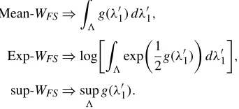
where= {λ′1;ε≤λ′1≤1−ε}for someε >0. HereT1′ (resp. λ′1)denotes a generic break date (resp. break fraction) used to construct a particular value of the Wald test, whereasT1(resp. λ1)will continue to denote the true break date (resp. break frac-tion). Given that the regressors are trending and the errors may have a unit root, none of these functionals need have any op-timal properties in our case. Nevertheless, given that they have some optimality properties in the stationary case, they are worth considering. Their limit distributions are a simple consequence of Theorem1, stated in the following corollary.
Corollary 1. Let g(λ′1) denote G0(λ′1) and G1(λ′1) for the
I(0)andI(1)cases, as defined in Theorem1. Then
Mean-WFS⇒
g(λ′1)dλ′1,
Exp-WFS⇒log
exp
1 2g(λ
′
1)
dλ′1 ,
sup-WFS⇒sup
g(λ′1).
Here things are not as simple as in the known break date case. Even though the distributions ofG0(λ′1)andG1(λ′1)are both chi-squared for any fixed λ′1, the two functions are different.
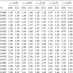
Accordingly, the limit distributions of the three tests differ in theI(0)andI(1)cases. Table1presents the asymptotic critical values with a value for the trimming parameter ε=0.01 and 0.15. These were calculated by simulations using iid N(0,1) random variables to approximate the Wiener process. The in-tegrals are approximated by normalized sums with 2000 steps, and 10,000 replications are used. What transpires from these re-sults is that although the limit distributions are different, the rel-evant quantiles are very similar for theI(0)andI(1)cases when considering the Exp functional. For example, for modelII, the 5% critical values withε=0.01 are 1.97 for theI(0)case and 2.02 for theI(1)case. Thus taking the larger critical value, cor-responding to 2.02, would be expected to bring a powerful ro-bust statistic for both stationary and integrated errors.
Table2 presents an extended grid of critical values for the Exp version of the test, which also includes a wider range of values for the trimming parameterε. From this table, we can deduce the asymptotic size of the test in both cases when the larger critical value is used. For example, for modelI, when do-ing a 5% test, the critical values are largest for the I(0)case, and in theI(1)case, the asymptotic size varies between 0.045 forε=0.25 and 0.035 forε=0.10. For modelII, the critical values are largest in theI(1)case, but in theI(0)case, the as-ymptotic size is between 0.045 and 0.05 for all values ofε. For modelIII, the relevant critical values correspond to those in the
I(1)case, in theI(0)case, the size is between 0.035 and 0.045. The discrepancies for other significance levels can be obtained from the table. Thus the minimum value of the size for theI(0) andI(1)cases is close to 5%, implying tests that are not very conservative, which is a useful feature to get decent power.
Remark 3. We computed the limit distribution of the test Exp-WFS under a sequence of local to unity alternatives (i.e.,
αT=1+c/Tforc<0) and verified that, as in the known break
date case, the test is conservative. Details are omitted.
Remark 4. We may be interested in using model III, and test only whether a shift in slope is present (β1withμ1 unre-stricted), that is, allow the possibility of both a shift in intercept
Table 1. Asymptotic distributions for one break occurring at an unknown date
ε=0.01 ε=0.15
sup-WFS Mean-WFS Exp-WFS sup-WFS Mean-WFS Exp-WFS
% I(0) I(1) I(0) I(1) I(0) I(1) I(0) I(1) I(0) I(1) I(0) I(1)
ModelI
0.900 9.99 ∞ 1.72 0.98 1.59 1.60 8.96 ∞ 1.31 0.70 1.22 1.26
0.950 11.64 ∞ 2.11 0.98 2.07 1.92 10.60 ∞ 1.64 0.70 1.74 1.58
0.975 13.08 ∞ 2.50 0.98 2.60 2.32 12.17 ∞ 1.98 0.70 2.30 1.99
0.990 15.03 ∞ 3.04 0.98 3.33 2.99 14.30 ∞ 2.47 0.70 3.12 2.64
ModelII
0.900 6.38 8.86 2.12 1.93 1.45 1.52 4.91 7.14 1.66 1.50 1.07 1.13 0.950 7.78 10.42 2.84 2.49 1.97 2.02 6.27 8.68 2.28 2.01 1.61 1.67 0.975 9.19 11.94 3.59 3.06 2.55 2.57 7.63 10.24 2.92 2.54 2.18 2.26 0.990 11.00 13.97 4.54 3.90 3.30 3.37 9.33 12.18 3.82 3.19 2.97 3.06 ModelIII
0.900 12.79 ∞ 3.36 2.91 2.68 2.96 11.11 ∞ 2.58 2.20 2.25 2.48
0.950 14.52 ∞ 4.16 3.47 3.34 3.55 12.86 ∞ 3.17 2.71 2.84 3.12
0.975 16.13 ∞ 4.96 4.04 3.94 4.15 14.38 ∞ 3.83 3.24 3.52 3.75
0.990 18.13 ∞ 6.11 4.88 4.67 5.02 16.66 ∞ 4.70 3.89 4.35 4.47
Table 2a. Asymptotic distribution of the Exp test: modelI
ε=0.01 ε=0.05 ε=0.10 ε=0.15 ε=0.25
% I(0) I(1) I(0) I(1) I(0) I(1) I(0) I(1) I(0) I(1)
0.900 1.59 1.60 1.47 1.52 1.33 1.41 1.22 1.26 0.83 0.91 0.905 1.60 1.61 1.51 1.55 1.36 1.43 1.26 1.28 0.86 0.93 0.910 1.62 1.62 1.56 1.57 1.40 1.45 1.30 1.30 0.90 0.96 0.915 1.66 1.65 1.59 1.59 1.44 1.46 1.35 1.34 0.93 0.98 0.920 1.71 1.67 1.63 1.62 1.50 1.49 1.40 1.36 0.98 1.01 0.925 1.76 1.70 1.67 1.65 1.55 1.52 1.46 1.40 1.03 1.04 0.930 1.81 1.74 1.71 1.69 1.59 1.55 1.50 1.43 1.09 1.08 0.935 1.85 1.78 1.75 1.72 1.66 1.58 1.56 1.47 1.15 1.11 0.940 1.92 1.81 1.82 1.76 1.72 1.62 1.61 1.51 1.20 1.16 0.945 1.98 1.86 1.89 1.82 1.80 1.66 1.69 1.56 1.28 1.21 0.950 2.07 1.92 1.97 1.86 1.88 1.70 1.74 1.58 1.33 1.26 0.955 2.14 1.97 2.05 1.92 1.96 1.76 1.85 1.67 1.41 1.33 0.960 2.22 2.04 2.16 1.99 2.05 1.82 1.93 1.73 1.51 1.40 0.965 2.33 2.11 2.25 2.07 2.18 1.88 2.02 1.81 1.61 1.49 0.970 2.44 2.23 2.40 2.16 2.30 1.98 2.14 1.88 1.73 1.58 0.975 2.60 2.32 2.53 2.29 2.45 2.07 2.30 1.99 1.92 1.68 0.980 2.74 2.50 2.69 2.41 2.60 2.19 2.50 2.14 2.11 1.81 0.985 3.02 2.81 2.90 2.60 2.79 2.39 2.74 2.36 2.35 2.01 0.990 3.33 2.99 3.24 2.81 3.05 2.67 3.12 2.64 2.83 2.32 0.995 3.91 3.62 3.84 3.26 3.60 3.29 3.55 3.28 3.33 2.91
and slope but only test if the latter is present. In that case, the limit distribution in the I(1)case is the same as in modelII. In theI(0)case, it is different but very close to that in theI(1) case, indeed even closer than for modelII. Thus we can still use the critical values corresponding to modelII.
Remark 5. The limit distribution of the Exp-WFSis still
sen-sitive to the Normality assumption on the errors whenα=1 in modelsIandIIIthat have a change in level. Size distortions occur when the distribution of the errors have fat tails so that
Table 2b. Asymptotic distribution of the Exp test: modelII
ε=0.01 ε=0.05 ε=0.10 ε=0.15 ε=0.25
% I(0) I(1) I(0) I(1) I(0) I(1) I(0) I(1) I(0) I(1)
0.900 1.45 1.52 1.34 1.40 1.20 1.28 1.07 1.13 0.71 0.74 0.905 1.47 1.58 1.38 1.45 1.24 1.33 1.11 1.19 0.74 0.79 0.910 1.51 1.62 1.42 1.49 1.29 1.36 1.15 1.23 0.79 0.84 0.915 1.55 1.65 1.47 1.53 1.32 1.41 1.19 1.27 0.83 0.89 0.920 1.60 1.70 1.53 1.57 1.37 1.46 1.24 1.32 0.87 0.93 0.925 1.64 1.74 1.58 1.62 1.43 1.51 1.30 1.37 0.92 0.98 0.930 1.70 1.80 1.64 1.68 1.47 1.57 1.34 1.44 0.97 1.02 0.935 1.76 1.86 1.70 1.73 1.54 1.62 1.39 1.49 1.03 1.08 0.940 1.84 1.92 1.76 1.78 1.61 1.69 1.47 1.53 1.11 1.14 0.945 1.89 1.98 1.84 1.86 1.68 1.78 1.54 1.59 1.19 1.22 0.950 1.97 2.02 1.90 1.93 1.75 1.86 1.61 1.67 1.25 1.28 0.955 2.06 2.10 1.98 2.01 1.85 1.93 1.71 1.73 1.32 1.37 0.960 2.19 2.19 2.07 2.10 1.94 2.05 1.80 1.80 1.40 1.46 0.965 2.30 2.29 2.19 2.23 2.06 2.14 1.91 1.91 1.52 1.59 0.970 2.41 2.46 2.29 2.36 2.19 2.24 2.06 2.10 1.65 1.73 0.975 2.55 2.57 2.42 2.51 2.34 2.39 2.18 2.26 1.81 1.84 0.980 2.74 2.82 2.61 2.71 2.56 2.55 2.42 2.39 1.97 2.02 0.985 3.00 3.09 2.83 2.98 2.79 2.81 2.64 2.61 2.20 2.24 0.990 3.30 3.37 3.07 3.27 3.20 3.18 2.97 3.06 2.60 2.61 0.995 3.88 4.01 3.61 3.95 3.80 3.68 3.62 3.46 3.28 3.27
Table 2c. Asymptotic distribution of the Exp test: modelIII
ε=0.01 ε=0.05 ε=0.10 ε=0.15 ε=0.25
% I(0) I(1) I(0) I(1) I(0) I(1) I(0) I(1) I(0) I(1)
0.900 2.68 2.96 2.51 2.82 2.35 2.65 2.25 2.48 1.86 2.15 0.905 2.70 2.98 2.56 2.86 2.39 2.70 2.27 2.53 1.90 2.20 0.910 2.74 3.00 2.60 2.90 2.45 2.74 2.31 2.57 1.96 2.25 0.915 2.81 3.02 2.65 2.94 2.50 2.79 2.36 2.63 2.01 2.29 0.920 2.85 3.07 2.71 3.00 2.56 2.83 2.40 2.67 2.06 2.35 0.925 2.92 3.12 2.75 3.05 2.62 2.87 2.46 2.76 2.11 2.41 0.930 2.99 3.17 2.82 3.11 2.68 2.93 2.53 2.83 2.18 2.47 0.935 3.05 3.23 2.89 3.17 2.74 2.98 2.59 2.90 2.26 2.54 0.940 3.12 3.32 2.97 3.24 2.79 3.03 2.66 2.97 2.35 2.62 0.945 3.22 3.40 3.04 3.30 2.88 3.10 2.74 3.05 2.43 2.69 0.950 3.34 3.55 3.12 3.36 2.98 3.16 2.84 3.12 2.50 2.79 0.955 3.37 3.60 3.23 3.46 3.10 3.25 2.92 3.20 2.62 2.88 0.960 3.50 3.66 3.36 3.57 3.22 3.34 3.03 3.32 2.76 3.01 0.965 3.63 3.77 3.46 3.68 3.33 3.44 3.14 3.47 2.89 3.15 0.970 3.76 3.93 3.63 3.81 3.48 3.59 3.30 3.60 3.06 3.31 0.975 3.94 4.15 3.83 3.99 3.67 3.77 3.52 3.75 3.24 3.50 0.980 4.13 4.28 4.06 4.15 3.86 4.00 3.62 3.96 3.46 3.69 0.985 4.44 4.54 4.39 4.42 4.11 4.29 3.92 4.23 3.73 4.06 0.990 4.67 5.02 4.78 4.76 4.57 4.59 4.35 4.47 4.04 4.57 0.995 5.55 5.72 5.42 5.42 5.15 5.16 5.02 5.25 4.78 5.58
outliers can be present. We do not consider this a defect of our suggested procedure. In the unit root case, levels shifts induced by exogenous events or by outliers are basically observation-ally equivalent. Thus if a test procedure is to have power for de-tecting exogenous level shifts, then it also must have increased probability of rejection when outliers occur. As we document later, the testing procedure ofVogelsang (2001)is such that the limit and finite-sample distributions are not sensitive to errors with a fat-tailed distribution; consequently, however, it also has no power for detecting exogenous level shifts. Thus either we reject for neither case or we reject for both cases. There seems to be no way around this problem. We prefer a procedure to in-dicate a rejection even if it is due to an outlier, because indeed such outliers acts as important level shifts.
The results also demonstrate that the Mean and Sup versions of the test are of little use in our context. Given the quite large discrepancies between the two sets of critical values, these tests would imply substantial size distortions in either theI(0)orI(1) case, depending on which case has the largest critical value. Some of the results in Table1can be explained using theoreti-cal arguments. First, for modelI, the limit of the Mean test in the
I(1)case is(1−2ε), or 0.98 forε=0.01 and 0.7 forε=0.15. The reason for this is that in large samples,WFS(λ′1)is
equiva-lent toe2
T′1+1/σ
2and thus the Mean test isT−1
WFS(λ′1)= (1−2ε)[(σ2(1−2ε)T)−1
e2T1′+1] +op(1)→
p(1−2ε),
using the fact that, from a standard law of large numbers,
[(1−2ε)T]−1
e2T1′+1→
pσ2. To explain why for theI(1) case the Sup version diverges in model I (the explanation is similar for modelIII), we again use the fact that in large sam-ples, WFS(λ′1) is equivalent to e2T′
1+1
/σ2. Thus the sup
sta-tistic is supe2T′ 1+1
/σ2=max{e2T′ 1+1
/σ2}. The probability of sup-WFS< η is Pr(∩ {e2T′
1+1
/σ2< η})=Pr(e2t/σ2<
η)(1−2ε)T using the assumption of independence; therefore, Pr(sup-WFS< η)→0 asT→ ∞if Pr(e2t/σ2< η) <1, which
is the case for anyη <∞. Thus sup-WFSdiverges to infinite as
T→ ∞.
2.5 Some Modifications to Improve Finite-Sample Properties
It is well known that the OLS estimate ofαis biased down-ward, especially when α is near 1. Thus in many cases, no truncation may apply when some truncation would be desir-able.Perron and Yabu (2009)recommended using a median-unbiased estimate. In the current context, however, obtaining an exactly median unbiased estimate is computationally very de-manding, especially in the unknown break date case and more so when a more general AR(p)structure for the noise com-ponent is entertained (as we do in Sec.4). An alternative ap-proach with similar finite-sample properties is the bias correc-tion proposed byRoy and Fuller (2001), which we adopt here. We consider that, based on the OLS estimate,Roy, Falk, and Fuller (2004)andPerron and Yabu (2009)used a similar bias-corrected estimate but based on a weighted symmetric least squares estimate ofα instead of the OLS estimate used here; both lead to tests with similar properties. It is a function of a unit root test, namely the t-ratio τˆ=(αˆ−1)/σˆα, whereαˆ is
the OLS estimate andσˆα is its standard deviation. The
bias-corrected estimate is given by
ˆ in the trend function [i.e., the number of elements in the vec-tor from model (1)],c2= [(1+r)T−τpct2 (Ip+T)][τpct(a+
τpct)(Ip+T)]−1,a is some constant, and τpct is a percentile
of the limit distribution of τˆ when α=1. The relevant limit distribution is that pertaining to the known break date case, be-cause the correction is applied to each given break fractions
T1′/T, and, accordingly, the critical values are those given by Perron (1989). We simulated the percentage points for each val-ues ofT1′/T, but we could use the values in the tables ofPerron (1989)with interpolation. In addition,Ip= [(p+1)/2], where
pis the order of the AR process considered for the noise com-ponent (here 1, but different in the generalizations considered in Sec.4). The parameters for which specific values need to be selected areτpct anda. Based on extensive simulation
ex-periments, we selecteda=10, because it leads to tests with better properties, and forτpct, we useτ0.95for the known break date case andτ0.99 for the unknown break date case (seeYabu 2005for details). Also, again based on extensive simulations, we found that the valued=1 for the truncation leads to the best results in finite samples. Thus our suggested procedure in-volves the following steps:
1. For any given break date, detrend the data by OLS to ob-tain residuals, sayuˆt.
5. Apply a GLS procedure withαˆMSto obtain the estimates
of the coefficients of the trend and the estimate of the variance of the residuals and construct the standard Wald-statistic, which we denote byWFMS.
6. When dealing with the case of an unknown break date, repeat steps 1–5 for all permissible break dates and con-struct the Exp-Wald statistic, denoted by Exp-WFMS.
Remark 6. Using the biased-corrected versions,αˆM, instead
of the OLS estimates does not change the stated large-sample results (Theorems 1 and Corollary 1). All that is needed for these asymptotic results to hold is thatT(αˆM−1)=Op(1)when
α=1, andT1/2(αˆM−α)→dN(0,1−α2)when|α|<1. These
conditions are satisfied.
3. SIMULATION EVIDENCE
In this section we assess the finite-sample properties of the procedure. We first consider the size of the tests. For this, we generate the data through a simple AR(1)process of the form
yt=αyt−1+et, with et∼iid N(0,1)andy0=0. (Setting the constant and trend parameters to zero is without loss of gen-erality, because the tests are invariant to them.) The nominal size of the tests is 5% throughout. We consider the following sample sizes: T =100,250,500 for a known break date and
T=100,250 for an unknown break date. The value of the trim-ming parameter for the Exp-WFMS test in the unknown break
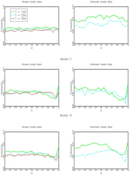
date case is set toε=0.01. The numbers of replications is 5,000 for the known break date case and 2000 for the unknown break date case. Using these specifications, we evaluate the size of the tests for values ofαin the range of[0,1]with increments of 0.05.
Figure1 presents the results. In the case of a known break date, the size of the test is very close to 5% for all values of the AR parameters in all cases considered even whenT=100. As expected, the test is slightly conservative for modelsIIandIII whenαis close to but not equal to 1. In the unknown break date case, the test shows some liberal size distortions whenT=100 and a change in intercept is involved (modelsI andIII). But these distortions are virtually eliminated whenT=250, except whenαis close to but not equal to 1, where the test is somewhat conservative, as expected.
We now consider the power of the tests. The specifications are the same, except that the data are generated by the following processes:
• For modelI:yt=ηDUt+ut
• For modelII:yt=ηDTt+ut
• For modelIII:yt=η(10DUt+DTt)+ut.
Figure 1. Finite sample size ofWFMStest.
Hereut=αut−1+et withet∼iid N(0,1)andu0=0. The break date is set toT1= [0.5T].
We compare the power of our test with that of three other tests: the Wald test based on the infeasible GLS estimates, which uses the true values ofαandT1, as well as theT−1WT
andPST tests ofVogelsang (2001)and the Exp version in the
unknown break case. We also experimented with the tests of Sayginsoy and Vogelsang (2004). Our simulations revealed that it is somewhat better than the test of Vogelsang (2001) for model I. For model II, it is not better than theT−1WT when
αis close to 1, and neither has better power thanPST whenα
is not close to 1. In addition, their test is not applicable to the
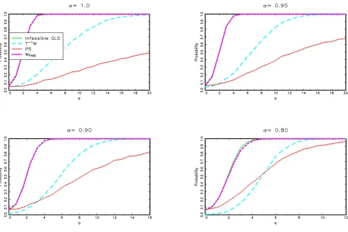
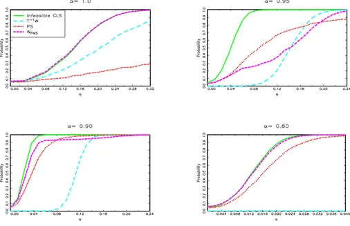
known break date case or to modelIIIwith an unknown break date. Thus here we report only comparisons with the original tests ofVogelsang (2001). For his tests, we use a 5% nominal size, and the comparisons should be made assuming that they are applied independently. The power curves are plotted for α=1.0,0.95,0.90, or 0.80 and a range of values ofη >0. We report raw non–size-adjusted power. With size-adjusted power, the qualitative results do not change appreciably, and all of the conclusions continue to hold. Note that our test is constructed assuming that the order of the autoregression is known to be 1. Thus the power may be overstated compared with what can be achieved in practice. However, as we show in Section4.3, our test continues to have good properties when no such knowledge is assumed and a nonparametric correction is applied.
First, consider Figure 2, which presents the results for model Iin the case of a known break date for T =100. For any values ofα, our test is as powerful as that based on the infeasible GLS regression that uses the true value of α. The test also is substantially more powerful than those ofVogelsang (2001). These results are quite remarkable, because our test (like any other) is inconsistent whenαis local to 1 (which is the case for the values ofαconsidered), because the intercept shift is then basically only an outlier. But an inconsistent test still can have decent power in finite samples. As expected, how-ever, power does not increase with the sample size but increases only with the magnitude of the change; accordingly, the results forT=250 and 500 are basically identical and are not reported here. The results for the case of an unknown break date, pre-sented in Figure3forT=100, yield similar conclusions, with
the exception that the power of our test is somewhat lower than what can be achieved with the infeasible GLS procedure. Still, power rises rapidly with the magnitude of the change.
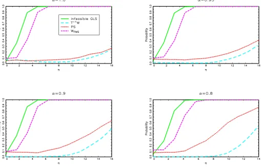
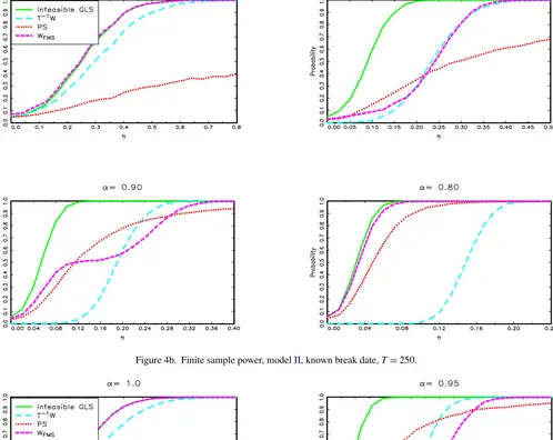
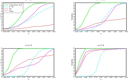
Now consider modelII. The power functions for the known break date case are presented in Figure 4, forT =100,250, and 500. Whenα=1, our test is as powerful as that based on the infeasible GLS estimates for anyT. Whenα=0.8,0.9, or 0.95 andT=100, the power of our test is lower, due largely to the fact that in this case the size is conservative. Nonetheless, it offers important power improvements over Vogelsang’s tests. AsTincreases, the power function of our test becomes closer to that of the infeasible GLS test. For instance, the power functions are equivalent whenT =500 and α=0.8 or 0.9. The power functions for the unknown break date case are presented in Fig-ure5, forT=100 and 250. The results are qualitatively similar, with the power functions being lower, as expected. Moreover, our test no longer globally dominates both theT−1W andPST
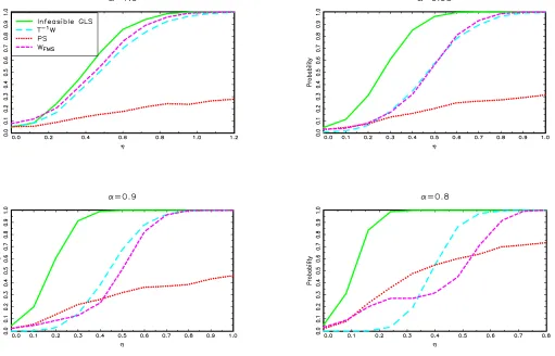
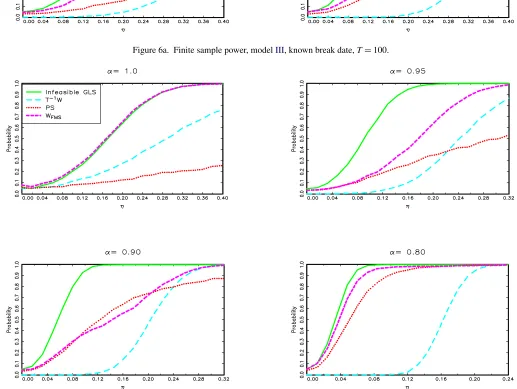
tests of Vogelsang (2001), though individually each of these tests has very poor power for some values of α. Figure 6for the known break date case and Figure7for the unknown break date case show that similar features hold for modelIII.
Remark 7. Our test is superior to Vogelsang’s PST test
in the unit root case is because it is defined by PST =
T−1/2Wzexp(−b∗JT), where Wz is the appropriate Wald test
constructed from a version of Equation (1) in which the vari-ables enter in the partial sum form. The componentJT is some
unit root test that converges to zero when the errors areI(0)and to some nondegenerate limit distribution when the errors are
Figure 2. Finite sample power, modelI, known break date,T=100.
Figure 3. Finite sample power of the Exp tests, modelI, unknown break date,T=100.
Figure 4a. Finite sample power, modelII, known break date,T=100.
Figure 4b. Finite sample power, modelII, known break date,T=250.
Figure 4c. Finite sample power, modelII, known break date,T=500.
Figure 5a. Finite sample power of the Exp tests, modelII, unknown break date,T=100.
Figure 5b. Finite sample power of the Exp tests, modelII, unknown break date,T=250.
Figure 6a. Finite sample power, modelIII, known break date,T=100.
Figure 6b. Finite sample power, modelIII, known break date,T=250.
Figure 6c. Finite sample power, modelIII, known break date,T=500.
Figure 7a. Finite sample power of the Exp tests, modelIII, unknown break date,T=100.
Figure 7b. Finite sample power of the Exp tests, modelIII, unknown break date,T=250.
I(1). The scalingb∗ is chosen such that the limit distribution of thePST test is the same in theI(1)andI(0)cases. Now the
originalT−1/2Wz has good properties in both cases. Because
PST is equivalent in large sample toT−1/2Wzin theI(0)case,
thePST test accordingly has good properties when the errors
areI(0). But things are different in theI(1)case, because the
PST test is then a randomized (or contaminated) version of the
Wz test, even in large samples. Thus the good properties of the
later are lost, and power is accordingly lower. Our procedure avoids this problem entirely. In both theI(0)andI(1)cases, in large samples our test is equivalent to the infeasible GLS test, which is the best possible in the known break date, which also translates into good properties in the unknown break case.
Overall, these results are very encouraging and point to the usefulness of our testing procedure. Next we extend them in two directions, first to allow a general serial correlation structure in the noise component, and then to allow more than one break.
4. GENERALIZATION OF THE ERROR COMPONENT
We now consider an extension of the analysis to the case where the error termutis allowed to have a more general
struc-ture. The data-generating process is now assumed to be given by (1) withutspecified by
ut=αut−1+υt,
(8) υt=d(L)et,
with d(L)=∞
i=0diLi, ∞i=0i|di|<∞, d(1)=0, and et∼
iid(0, σ2). Again, we assume for simplicity that u0 is some constant. These conditions imply that the following func-tional central limit theorem holds for the partial sums of υt:
T−1/2[rT]
t=1υt⇒σd(1)W(r). Under the stated conditions,ut has an AR representation, say A(L)ut =et, where A(L)=
1−∞
i=1aiLi. In the representation (8), we wish to have the
parameterαrepresent the sum of the AR coefficients. Accord-ingly, we have the representation
ut=αut−1+A∗(L) ut−1+et
withA∗(L)=∞
i=0a∗iLi, wherea∗i = −
∞
j=i+1aj.
4.1 Estimation ofα
Becauseαrepresents the sum of the AR coefficients, we can-not use the estimate (2) based on an autoregression of order 1, because it is inconsistent forα when the errors ut are a
gen-eralI(0)process. Instead, we base our estimate on a truncated autoregression of orderk. Letuˆtbe the residuals from a
regres-sion ofytonxt;then the estimate ofαconsidered is the OLS
estimateα˜ obtained from the regression
ˆ
ut=αuˆt−1+
k
i=1
ζi uˆt−i+etk, (9)
when ut isI(0),T1/2(α˜−α)=Op(1). In contrast, ifα=1+
c/T, thenT(α˜ −1)⇒c+d(1)1
0Jc∗(r)dW(r)/
1
0 Jc∗(r)2dr,
whereJc∗(r)is the residual function from a regression ofJc(r)≡
r
0exp(c(r−s))dW(s) on the continuous-time version of the deterministic components. We also use the same bias correction for the least squares estimate,α˜M, as described in Section2.5,
with the same specifications, and apply the truncation (4) with
˜
αMinstead ofαˆ. The truncated version of the bias-corrected
es-timate,α˜MS, is still super-efficient under a local unit root, that is,
T(α˜MS−1)→p0 whenα=1+c/T. As usual, the consistency
ofα˜ and the truncated bias-corrected version,α˜MS, depends on
having the AR approximationkincrease at a suitable rate asT
increases, namelyk→ ∞andk3/T→0 asT→ ∞(seeBerk 1974). We suggest using an information criterion such as the Bayes information criterion (BIC) to ensure that these proper-ties are satisfied.
4.2 The Test Statistics
The estimate of considered is a quasi-FGLS estimate as-suming AR(1)errors, that is, the OLS estimate in the trans-formed regression,
(1− ˜αMSL)yt=(1− ˜αMSL)x′t+(1− ˜αMSL)ut, (10)
for t=2, . . . ,T, together withy1=x′1+u1. Denote the re-sulting estimates by˜. The specific form of the Wald test de-pends on the nature of the errors,I(0)or I(1), and the model. First, consider theI(0)case. For any of the three models, we simply need to replace s2 in (5) by hˆυ, an estimate of (2π
times) the spectral density function at frequency zero ofυt=
(1−αL)ut. We denote the resulting Wald test byWRQF(λ1), where the subscript “RQF” stands for robust quasi-FGLS; more precisely, on a weighted sum of the autocovariances given by
ˆ
are the OLS residuals from the regression (10). The quadratic spectral window is used, withmselected according to the “plug-in method” advocated byAndrews (1991)using an AR(1) ap-proximation. The other estimate considered is an AR spectral density estimate (at frequency zero). The residuals from the re-gression (10) are(1− ˜αSL)ut, and thus in large samples, they
whereeˆtkare the corresponding OLS residuals. The estimate is
then for the construction of the AR spectral density estimate. With α=1, in large samples,(1− ˜αMSL)utis equivalent toυt= ut,
and this estimate can be obtained from the regression
ˆ in intercept is involved, things are somewhat more complex. For modelIII, the limit distribution of the statisticWRQF(λ1) defined by (11) is
ond component, but the first component involves two complica-tions. The first complication is thathυis not the proper scaling;
instead, we needσυ2=var(υt)to haveυ[2λ
1T]+1/σ 2
υ beχ2(1).
The second complication is thatυ[2λ
1T]is not iid as in the case of the AR(1)specification. This matters because the limit distribu-tion of the test with an unknown break date will differ from that tabulated earlier. Now recall that˜ =(μ0,˜ μ1,˜ β0)˜ ′for modelI and ˜ =(μ0,˜ μ1,˜ β0,˜ β1)˜ ′ for model III. To achieve the de-sired corrections, we need to replaceμ1˜ byμ∗1, which requires two modifications. The first is to get backe2[λ
1T]+1instead of υ[2λ
1T]+1in the limit distribution. Denote the sequence of esti-matesμ˜1for different values of the break dateT1byμ˜1(T1)for
in large samples. The second modification is to ensure the proper scaling. To that effect, we defineμ∗1= ˆhυ1/2ζ (ˆ L)μ1(˜ T1)/ case of modelIwith hypothesis testing pertaining only to the shift in interceptμ1, the statistic reduces to, withR= [0,1,0],
WRQF∗ (λ1)=(μ∗1)2/[ˆhυR(X′X)−1R′]
=(ζ (ˆ L)μ1(˜ T1)/σˆek2)/[R(X′X)−1R′]
and the estimatehˆυ is not needed.
Again, the decision rule to select whether to use the form of the statistic corresponding to theI(0)orI(1)case depends on whether or not the truncated value α˜MS is 1. Asymptotically,
this results in a correct classification and a consistent testing procedure. Thus we recommend the following procedure:
1. Detrend the data by OLS to obtain residualsuˆt.
2. Consider the autoregression (9) withkselected using an information criterion; we recommend the BIC, withk al-lowed to be in the range[0,12(T/100)1/4](seeSchwarz 1978). The corresponding estimate is denoted α˜. If the order selected is k=0, then the procedure described in Section2.5applies; otherwise, the next steps are applied. 3. Construct the bias-corrected version ofα,˜ α˜M, as defined
by (7) described in Section2.5. Then apply the truncation
˜
αMS=
˜
αM if| ˜αM−1|>T−1/2
1 if| ˜αM−1| ≤T−1/2.
4. Apply the quasi-GLS procedure withα˜MS to obtain the
estimate of and construct the Wald-statisticWRQF or
WRQF∗ depending on the model and value of α˜MS, using
one of the two versions ofhˆυ suggested to construct the
estimate of (2πtimes) the spectral density function at fre-quency zero ofυt.
5. With an unknown break, the test statistic needs to be eval-uated for each break date candidate and the Exp functional defined by (6) is evaluated.
4.3 Finite-Sample Simulations
Here we present results about the finite-sample size and power of our test with an AR(2)error component generated by
ut=αut−1+ψ (ut−1−ut−2)+et, (14)
whereet∼iid N(0,1)andu0=u−1=0. The number of repli-cations is 1000, and we assess the size properties of our test at the nominal 5% level for the following specifications:α=
1,0.95,0.90,0.80; ψ =0.0,0.3,0.5,0.7; and T =100. We consider positive AR coefficients, because this is the most rele-vant case in practice.
We consider three versions of our test that varies with the choice ofhˆυ. In the first case, the estimate (12) is used and is
referred to as “NP” (for Non Parametric). The second is the AR based estimates withkchosen byBIC. It is referred to as “AR” (for AR). The third is a mixture of NP and AR. We use NP for the case| ˜αMS|<1 and AR forα˜MS=1. It is referred to “AN”
(for AR and Non Parametric). Note that in the case of modelI, whenα˜MS=1 we do not have to estimate the long-run variance.
Therefore, AN is the same as NP.
Consider first the case with a known break date. Table 3 presents the size of the tests. The results suggest that the “AR” version can have serious size distortions in some of the I(0) cases considered and that the “NP” specifications in turn leads to size distortions in theI(1)case. Overall, the mixed method “AN” is a good compromise and has acceptable size proper-ties, though somewhat conservative when α is close to but not equal to 1. We now consider the power of our test with a break occurring at midsample, i.e., T1= [0.5T]. We con-sider only the specification that uses the mixed method “AN” to estimatehυ and compare its properties with theT−1WT and
thePST tests ofVogelsang (2001), again using a 5% nominal
size so that their properties pertain to the case when both tests
Table 3. Finite sample null rejection probability ofWRQFwith 5%
nominal size,T=100, known break date AR(2)case: ut=αut−1+ψ (ut−1−ut−2)+et
ModelI ModelII ModelIII
α ψ AR AN AR NP AN AR NP AN
1.00 0.00 0.06 0.06 0.09 0.08 0.10 0.08 0.09 0.09 0.30 0.07 0.06 0.12 0.12 0.10 0.08 0.11 0.09 0.50 0.05 0.06 0.10 0.13 0.09 0.10 0.12 0.09 0.70 0.04 0.07 0.10 0.17 0.12 0.10 0.14 0.11
0.95 0.00 0.07 0.08 0.04 0.04 0.05 0.06 0.05 0.05 0.30 0.07 0.05 0.04 0.03 0.03 0.05 0.04 0.04 0.50 0.07 0.05 0.03 0.01 0.02 0.04 0.03 0.03 0.70 0.06 0.07 0.02 0.01 0.01 0.03 0.02 0.02
0.90 0.00 0.06 0.08 0.04 0.04 0.03 0.05 0.05 0.05 0.30 0.07 0.05 0.04 0.03 0.03 0.05 0.04 0.04 0.50 0.08 0.05 0.05 0.01 0.02 0.05 0.03 0.03 0.70 0.10 0.04 0.07 0.01 0.01 0.07 0.02 0.02
0.80 0.00 0.07 0.07 0.05 0.05 0.07 0.07 0.06 0.06 0.30 0.08 0.05 0.06 0.03 0.03 0.07 0.04 0.04 0.50 0.10 0.03 0.07 0.02 0.02 0.10 0.03 0.03 0.70 0.18 0.06 0.10 0.03 0.04 0.18 0.04 0.04
are applied independently. Table4 presents the power results forη=0,0.1,0.3,0.5. Our test again has good properties and dominates the others for all models and values ofαandψ.
Table5 shows the size properties of our test in the case of an unknown break date when the Exp functional is used. The results suggest again that the mixed method “AN” to estimate
hυis preferable. The test based on the “AR” specification is too
liberal especially when α=0.8,0.9, and ψ >0, and the test based on the “NP” specification is too liberal whenα=1 and ψ >0. Next, we consider the power of our test with the “AN” specification. We only consider the Exp versions of theT−1WT
and thePST tests ofVogelsang (2001)as they work best for all
models (compared with the Mean and Sup functionals). Table6 presents the power results forη=0,0.1,0.3,0.5. Our test again dominates the others in most cases. For models IandIII, our test is considerably superior and for modelII, it is competitive to the best of theT−1WT andPST tests.
5. THE MULTIPLE BREAKS CASE
Our testing procedure extends, in principle, naturally to the case of multiple breaks. This is important since, as discussed inPerron (2006), most tests may exhibit non monotonic power functions if the number of breaks present under the alternative is greater than the number of breaks explicitly accounted for in the construction of the tests. Consider the following extended versions of our three models formbreaks denoted (T1, . . . ,Tm)
with corresponding break fractionsλi=Ti/T (i=1, . . . ,m).
Model I (Multiple structural breaks in intercepts). xt=(1,
DU1t, . . . ,DUmt,t)′,=(μ0, μ1, . . . , μm, β0)′whereDUit=
1(t>Ti). The hypothesis of interest isμ1= · · · =μm=0.
Model II (Multiple structural breaks in slopes). xt =(1,t,
DT1t, . . . ,DTmt,)′, =(μ0, β0, β1, . . . , βm)′ where DTit =
1(t >Ti)(t−Ti). The hypothesis of interest is β1 = · · · =
βm=0.
Table 4. Finite sample power, known break date,T=100, AR(2)case:ut=αut−1+ψ (ut−1−ut−2)+et
ModelI ModelII ModelIII
α ψ η PS T−1W WRQF PS T−1W WRQF PS T−1W WRQF
1.00 0.00 0.10 0.04 0.05 0.18 0.05 0.07 0.11 0.06 0.08 0.20
0.30 0.08 0.14 0.85 0.11 0.24 0.35 0.12 0.27 0.90
0.50 0.12 0.28 1.00 0.17 0.54 0.71 0.20 0.60 1.00
0.30 0.10 0.03 0.06 0.18 0.04 0.09 0.12 0.04 0.08 0.19
0.30 0.05 0.10 0.84 0.06 0.17 0.23 0.06 0.17 0.85
0.50 0.07 0.19 1.00 0.09 0.34 0.45 0.11 0.40 1.00
0.50 0.10 0.03 0.06 0.19 0.03 0.08 0.10 0.02 0.09 0.17
0.30 0.03 0.09 0.84 0.03 0.13 0.17 0.03 0.15 0.83
0.50 0.04 0.15 1.00 0.05 0.23 0.31 0.05 0.29 1.00
0.70 0.10 0.01 0.07 0.19 0.01 0.11 0.11 0.01 0.13 0.18
0.30 0.01 0.09 0.86 0.02 0.13 0.14 0.02 0.16 0.81
0.50 0.02 0.12 1.00 0.02 0.16 0.21 0.02 0.20 1.00
0.95 0.00 0.10 0.07 0.05 0.20 0.05 0.02 0.07 0.05 0.02 0.18
0.30 0.10 0.15 0.86 0.14 0.21 0.34 0.16 0.24 0.87
0.50 0.18 0.33 1.00 0.28 0.65 0.77 0.27 0.70 1.00
0.30 0.10 0.05 0.05 0.17 0.03 0.01 0.05 0.03 0.01 0.13
0.30 0.08 0.11 0.82 0.07 0.09 0.17 0.08 0.09 0.84
0.50 0.12 0.21 0.99 0.16 0.35 0.50 0.16 0.41 1.00
0.50 0.10 0.05 0.04 0.18 0.01 0.00 0.02 0.02 0.01 0.10
0.30 0.06 0.08 0.82 0.04 0.04 0.10 0.05 0.03 0.78
0.50 0.09 0.14 0.99 0.10 0.17 0.23 0.10 0.18 1.00
0.70 0.10 0.04 0.04 0.18 0.00 0.00 0.02 0.00 0.00 0.08
0.30 0.05 0.05 0.81 0.02 0.01 0.04 0.02 0.01 0.72
0.50 0.05 0.08 0.99 0.04 0.04 0.09 0.03 0.04 0.99
0.90 0.00 0.10 0.08 0.04 0.19 0.06 0.00 0.09 0.08 0.00 0.15
0.30 0.15 0.16 0.83 0.27 0.23 0.33 0.26 0.21 0.89
0.50 0.29 0.41 1.00 0.43 0.79 0.85 0.43 0.82 1.00
0.30 0.10 0.07 0.03 0.16 0.04 0.00 0.06 0.04 0.00 0.12
0.30 0.13 0.09 0.81 0.17 0.07 0.24 0.17 0.07 0.83
0.50 0.21 0.23 0.99 0.33 0.48 0.55 0.34 0.50 1.00
0.50 0.10 0.06 0.02 0.16 0.02 0.00 0.04 0.03 0.00 0.10
0.30 0.09 0.05 0.76 0.13 0.02 0.21 0.13 0.02 0.76
0.50 0.16 0.14 0.99 0.29 0.22 0.37 0.26 0.22 1.00
0.70 0.10 0.04 0.00 0.14 0.02 0.00 0.04 0.01 0.00 0.08
0.30 0.07 0.02 0.66 0.08 0.00 0.20 0.07 0.00 0.72
0.50 0.13 0.06 0.95 0.23 0.04 0.35 0.18 0.03 0.99
0.80 0.00 0.10 0.09 0.01 0.18 0.12 0.00 0.22 0.15 0.00 0.24
0.30 0.28 0.15 0.85 0.60 0.30 0.53 0.58 0.28 0.90
0.50 0.54 0.54 1.00 0.81 0.97 0.92 0.81 0.98 1.00
0.30 0.10 0.07 0.00 0.15 0.11 0.00 0.17 0.11 0.00 0.21
0.30 0.24 0.07 0.77 0.56 0.09 0.59 0.54 0.07 0.89
0.50 0.49 0.32 1.00 0.83 0.83 0.81 0.76 0.79 1.00
0.50 0.10 0.06 0.00 0.10 0.09 0.00 0.16 0.08 0.00 0.17
0.30 0.20 0.03 0.64 0.58 0.02 0.72 0.55 0.01 0.91
0.50 0.46 0.18 0.97 0.85 0.52 0.84 0.78 0.43 1.00
0.70 0.10 0.04 0.00 0.11 0.08 0.00 0.21 0.04 0.00 0.19
0.30 0.15 0.00 0.55 0.61 0.00 0.86 0.52 0.00 0.94
0.50 0.35 0.05 0.94 0.89 0.09 0.94 0.81 0.08 1.00
Table 5. Finite sample null rejection probability of Exp-WRQFwith
5% nominal size,T=100, unknown break date AR(2)case: ut=αut−1+ψ (ut−1−ut−2)+et
ModelI ModelII ModelIII
α ψ AR AN AR NP AN AR NP AN
1.00 0.00 0.09 0.09 0.09 0.09 0.11 0.10 0.10 0.10 0.30 0.10 0.07 0.14 0.18 0.13 0.13 0.14 0.11 0.50 0.08 0.05 0.13 0.16 0.13 0.12 0.18 0.11 0.70 0.03 0.05 0.14 0.26 0.13 0.18 0.27 0.15
0.95 0.00 0.10 0.09 0.04 0.03 0.03 0.05 0.05 0.07 0.30 0.08 0.08 0.05 0.04 0.03 0.07 0.04 0.04 0.50 0.09 0.06 0.03 0.04 0.03 0.06 0.03 0.03 0.70 0.08 0.04 0.04 0.02 0.01 0.04 0.04 0.01
0.90 0.00 0.10 0.10 0.02 0.03 0.02 0.05 0.05 0.04 0.30 0.12 0.09 0.04 0.03 0.02 0.08 0.03 0.03 0.50 0.11 0.06 0.05 0.02 0.01 0.08 0.03 0.02 0.70 0.19 0.04 0.13 0.05 0.02 0.15 0.03 0.02
0.80 0.00 0.14 0.11 0.04 0.03 0.04 0.07 0.06 0.05 0.30 0.17 0.08 0.06 0.02 0.03 0.10 0.03 0.04 0.50 0.26 0.05 0.12 0.02 0.03 0.19 0.02 0.04 0.70 0.71 0.09 0.31 0.08 0.08 0.57 0.08 0.09
Model III(Multiple structural breaks both in intercepts and slopes). xt = (1,DU1t, . . . ,DUmt,t,DT1t, . . . ,DTmt)′, =
(μ0, μ1, . . . , μm, β0, β1, . . . , βm)′. The hypothesis of interest is
μ1= · · · =μm=β1= · · · =βm=0.
All theoretical results discussed for the case of a single break continue to hold with minor modifications, as stated in the fol-lowing theorem.
Theorem 3. Consider first the case of known break dates. Let
WFS(λ)denote the Wald test for testing the relevant null
hypoth-esis. Under the data-generating process (1), when|α|<1, the results of Theorem1 continue to hold with F(r, λ1)replaced by the following: for model I, F(r, λ1, . . . , λm)= [1,1(r >
In addition, the Exp-test, defined by
Exp-WFS=log tion of the Wald test.
Remark 8. BecauseQ(λ)∼N(0,H(λ)),R∗H(λ)−1Q(λ)∼
N(0,R∗H(λ)−1R∗′)and V2(λ) is a chi-squared random vari-able withmdegrees of freedom that is independent ofV1(λ). It is also easy to see that whenm=1, we recover the results of Theorem1.
Although the theoretical extensions to the case with multiple breaks are straightforward, there remains an important problem for practical implementations. The reason is that the Exp-WFS,
and the Mean and Sup versions, depend on Wald tests evalu-ated at a number of partitions (or combinations of break dates) of order O(Tm). This becomes prohibitive for common sam-ple sizes oncemexceeds 2. For the Sup-Wald test, an efficient solution for finding the partition that corresponds to the maxi-mal value of the Wald test has been devised based on a dynamic programming algorithm (seeBai and Perron 2003); however, no such efficient algorithm exists to compute the Mean and Exp-Wald tests in the case of multiple breaks. Thus a full treatment will need to await advances in this respect. Nevertheless, the case with two breaks is computationally feasible and also im-portant in practice. For example,Lumsdaine and Papell (1997) provided evidence that the data of Nelson and Plosser (1982) may have two breaks in a trend function. To that effect, Ta-ble7presents the relevant quantiles of the limiting distributions of the Exp-WFStest statistic for both the I(0)andI(1)cases.
Again, the largest of these cases should be used to perform hy-pothesis testing. Note that here also the test is only slightly con-servative (asymptotically) for the cases that do not correspond to that from which the critical values are selected.
6. EMPIRICAL APPLICATIONS
This section considers empirical applications related to real GDP series for several countries. As discussed in Section1, as-sessing the stability of the trend function of series of aggregate economic activity is an important practical question. We present evidence using different sets of series. The first set comprises historical series for various countries spanning the period 1870– 1986 and considers both real GDP series and their per capita counterparts. The second set considers postwar real GDP series for the G7 countries.
6.1 Historical Real GDP Series
We consider a historical data set of (log) real GDP series and their per capita counterparts from 1870–1986 for 10 differ-ent countries: Australia, Canada, Denmark, France, Germany, Italy, Norway, Sweden, the United Kingdom, and the United States. This data set, used previously byKormendi and Meguire (1990), Perron (1992), and Perron and Zhu (2005), was ob-tained through theJournal of Money, Credit and Banking’s ed-itorial office. All series are real GDP except that the United
Table 6. Finite sample power, unknown break date,T=100, AR(2)case:ut=αut−1+ψ (ut−1−ut−2)+et
ModelI ModelII ModelIII
α ψ η PS T−1W WRQF PS T−1W WRQF PS T−1W WRQF
1.00 0.00 0.10 0.05 0.06 0.08 0.06 0.06 0.12 0.06 0.08 0.15
0.30 0.04 0.04 0.36 0.10 0.24 0.29 0.11 0.24 0.52
0.50 0.06 0.04 0.92 0.16 0.53 0.59 0.17 0.49 0.98
0.30 0.10 0.04 0.09 0.06 0.05 0.08 0.14 0.03 0.09 0.15
0.30 0.04 0.07 0.37 0.05 0.15 0.25 0.05 0.16 0.43
0.50 0.03 0.08 0.92 0.07 0.36 0.41 0.10 0.32 0.94
0.50 0.10 0.01 0.11 0.07 0.02 0.10 0.12 0.02 0.10 0.10
0.30 0.03 0.11 0.37 0.03 0.14 0.16 0.02 0.14 0.38
0.50 0.02 0.10 0.91 0.04 0.27 0.28 0.04 0.29 0.95
0.70 0.10 0.01 0.18 0.05 0.02 0.14 0.14 0.01 0.14 0.15
0.30 0.01 0.17 0.36 0.02 0.16 0.18 0.01 0.17 0.41
0.50 0.01 0.17 0.96 0.02 0.25 0.21 0.02 0.24 0.93
0.95 0.00 0.10 0.08 0.02 0.10 0.04 0.01 0.05 0.06 0.01 0.08
0.30 0.07 0.01 0.38 0.11 0.15 0.17 0.11 0.14 0.42
0.50 0.07 0.01 0.91 0.21 0.58 0.56 0.23 0.53 0.98
0.30 0.10 0.06 002 0.10 0.02 0.01 0.06 0.02 0.01 0.06
0.30 0.05 0.01 0.35 0.06 0.06 0.12 0.07 0.06 0.32
0.50 0.04 0.01 0.90 0.13 0.32 0.29 0.15 0.30 0.95
0.50 0.10 0.03 0.01 0.07 0.01 0.01 0.02 0.01 0.01 0.03
0.30 0.03 0.01 0.33 0.03 0.02 0.05 0.05 0.03 0.24
050 0.03 0.01 0.90 0.07 0.14 0.10 0.09 0.12 0.88
0.70 0.10 0.02 0.00 0.04 0.01 0.00 0.02 0.01 0.00 0.02
0.30 0.02 0.00 0.30 0.01 0.00 0.03 0.01 0.00 0.17
0.50 0.03 0.00 0.91 0.04 0.03 0.05 0.03 0.02 0.82
0.90 0.00 0.10 0.09 0.00 0.09 0.05 0.00 0.05 0.07 0.00 0.07
0.30 0.07 0.00 0.35 0.19 0.14 0.13 0.22 0.13 0.44
0.50 0.08 0.00 0.92 0.30 0.70 0.51 0.36 0.59 0.98
0.30 0.10 0.04 0.00 0.08 0.02 0.00 0.04 0.04 0.00 0.05
0.30 0.05 0.00 0.33 0.12 0.03 0.10 0.13 0.04 0.30
0.50 0.05 0.00 0.88 0.25 0.34 0.28 0.25 0.29 0.95
0.50 0.10 0.03 0.00 0.06 0.02 0.00 0.02 0.02 0.00 0.02
0.30 0.04 0.00 0.30 0.11 0.01 0.12 0.13 0.01 0.26
0.50 0.03 0.00 0.86 0.21 0.11 0.16 0.21 0.08 0.88
0.70 0.10 0.02 0.00 0.04 0.01 0.00 0.04 0.01 0.00 0.02
0.30 0.02 0.00 0.24 0.06 0.00 0.15 0.06 0.00 0.20
0.50 0.02 0.00 0.77 0.18 0.01 0.25 0.15 0.01 0.81
0.80 0.00 0.10 0.08 0.00 0.11 0.09 0.00 0.12 0.13 0.00 0.13
0.30 0.07 0.00 0.36 0.19 0.14 0.26 0.48 0.09 0.54
0.50 0.16 0.00 0.89 0.65 0.91 0.50 0.65 0.80 0.98
0.30 0.10 0.05 0.00 0.09 0.06 0.00 0.09 0.09 0.00 0.10
0.30 0.06 0.00 0.29 0.12 0.02 0.37 0.44 0.02 0.51
0.50 0.08 0.00 0.86 0.61 0.58 0.50 0.63 0.46 0.96
0.50 0.10 0.03 0.00 0.05 0.06 0.00 0.08 0.07 0.00 0.08
0.30 0.04 0.00 0.16 0.11 0.00 0.51 0.45 0.00 0.61
0.50 0.06 0.00 0.70 0.69 0.22 0.67 0.63 0.14 0.94
0.70 0.10 0.01 0.00 0.08 0.04 0.00 0.17 0.04 0.00 0.18
0.30 0.02 0.00 0.16 0.06 0.00 0.76 0.41 0.00 0.65
0.50 0.03 0.00 0.54 0.74 0.02 0.91 0.70 0.00 0.96