4
FUZZY CLUSTERING
Clustering techniques are mostly unsupervised methods that can be used to organize data into groups based on similarities among the individual data items. Most clustering algorithms do not rely on assumptions common to conventional statistical methods, such as the underlying statistical distribution of data, and therefore they are useful in situations where little prior knowledge exists. The potential of clustering algorithms to reveal the underlying structures in data can be exploited in a wide variety of appli-cations, including classification, image processing, pattern recognition, modeling and identification.
This chapter presents an overview of fuzzy clustering algorithms based on the c-means functional. Readers interested in a deeper and more detailed treatment of fuzzy clustering may refer to the classical monographs by Duda and Hart (1973), Bezdek (1981) and Jain and Dubes (1988). A more recent overview of different clustering algorithms can be found in (Bezdek and Pal, 1992).
4.1 Basic Notions
The basic notions of data, clusters and cluster prototypes are established and a broad overview of different clustering approaches is given.
4.1.1 The Data Set
tive data is considered. The data are typically observations of some physical process. Each observation consists of n measured variables, grouped into an n-dimensional column vectorzk = [z1k, . . . , znk]T,zk ∈ Rn. A set ofN observations is denoted by
In the pattern-recognition terminology, the columns of this matrix are calledpatterns or objects, the rows are called thefeaturesor attributes, andZis called thepatternor data matrix. The meaning of the columns and rows ofZdepends on the context. In medical diagnosis, for instance, the columns ofZmay represent patients, and the rows are then symptoms, or laboratory measurements for these patients. When clustering is applied to the modeling and identification of dynamic systems, the columns of Z may contain samples of time signals, and the rows are, for instance, physical variables observed in the system (position, pressure, temperature, etc.). In order to represent the system’s dynamics, past values of these variables are typically included inZas well.
4.1.2 Clusters and Prototypes
Various definitions of a cluster can be formulated, depending on the objective of clus-tering. Generally, one may accept the view that a cluster is a group of objects that are more similar to one another than to members of other clusters (Bezdek, 1981; Jain and Dubes, 1988). The term “similarity” should be understood as mathematical similarity, measured in some well-defined sense. In metric spaces, similarity is often defined by means of a distance norm. Distance can be measured among the data vectors them-selves, or as a distance from a data vector to someprototypical object(prototype) of the cluster. The prototypes are usually not known beforehand, and are sought by the clustering algorithms simultaneously with the partitioning of the data. The prototypes may be vectors of the same dimension as the data objects, but they can also be de-fined as “higher-level” geometrical objects, such as linear or nonlinear subspaces or functions.
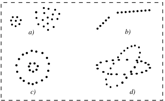
Data can reveal clusters of different geometrical shapes, sizes and densities as demonstrated in Figure 4.1. While clusters (a) are spherical, clusters (b) to (d) can be characterized as linear and nonlinear subspaces of the data space. The performance of most clustering algorithms is influenced not only by the geometrical shapes and den-sities of the individual clusters, but also by the spatial relations and distances among the clusters. Clusters can be well-separated, continuously connected to each other, or overlapping each other.
4.1.3 Overviewof Clustering Methods
c)
a) b)
d)
Figure 4.1. Clusters of different shapes and dimensions in R2. After (Jainand Dubes, 1988).
Hard clusteringmethods are based on classical set theory, and require that an object either does or does not belong to a cluster. Hard clustering means partitioning the data into a specified number of mutually exclusive subsets.
Fuzzy clusteringmethods, however, allow the objects to belong to several clusters simultaneously, with different degrees of membership. In many situations, fuzzy clus-tering is more natural than hard clusclus-tering. Objects on the boundaries between several classes are not forced to fully belong to one of the classes, but rather are assigned membership degrees between 0 and 1 indicating their partial membership. The dis-crete nature of the hard partitioning also causes difficulties with algorithms based on analytic functionals, since these functionals are not differentiable.
Another classification can be related to the algorithmic approach of the different techniques (Bezdek, 1981).
Agglomerative hierarchical methods andsplitting hierarchical methods form new clusters by reallocating memberships of one point at a time, based on some suitable measure of similarity.
Withgraph-theoretic methods, Zis regarded as a set of nodes. Edge weights be-tween pairs of nodes are based on a measure of similarity bebe-tween these nodes. Clustering algorithms may use anobjective functionto measure the desirability of partitions. Nonlinear optimization algorithms are used to search for local optima of the objective function.
The remainder of this chapter focuses on fuzzy clustering with objective function. These methods are relatively well understood, and mathematical results are available concerning the convergence properties and cluster validity assessment.
4.2 Hard and Fuzzy Partitions
possi-bilistic partitions can be seen as a generalization ofhard partitionwhich is formulated in terms of classical subsets.
4.2.1 Hard Partition
The objective of clustering is to partition the data setZintocclusters (groups, classes). For the time being, assume thatc is known, based on prior knowledge, for instance. Using classical sets, a hard partition of Z can be defined as a family of subsets
{Ai|1≤i≤c} ⊂ P(Z)1with the following properties (Bezdek, 1981):
Equation (4.2a) means that the union subsets Ai contains all the data. The subsets
must be disjoint, as stated by (4.2b), and none of them is empty nor contains all the data inZ(4.2c). In terms ofmembership (characteristic) functions, a partition can be conveniently represented by thepartition matrixU = [µik]c×N. Theith row of this
matrix contains values of the membership functionµi of the ith subsetAi of Z. It
follows from (4.2) that the elements ofUmust satisfy the following conditions: µik ∈ {0,1}, 1≤i≤ c, 1≤k ≤N, (4.3a)
The space of all possible hard partition matrices for Z, called the hard partitioning space (Bezdek, 1981), is thus defined by
Mhc =
Example 4.1 Hard partition.Let us illustrate the concept of hard partition by a sim-ple examsim-ple. Consider a data setZ={z1,z2, . . . ,z10}, shown in Figure 4.2.
A visual inspection of this data may suggest two well-separated clusters (data points z1toz4andz7toz10respectively), one point in between the two clusters (z5), and an “outlier”z6. One particular partitionU∈ Mhcof the data into two subsets (out of the
z1
z3
z4 z5
z6
z7
z8
z10
z9
z2
Figure 4.2. A data set in R2.
210possible hard partitions) is
U=
-1 1 1 1 1 1 0 0 0 0
0 0 0 0 0 0 1 1 1 1
. .
The first row ofUdefines point-wise the characteristic function for the first subset of Z,A1, and the second row defines the characteristic function of the second subset ofZ, A2. Each sample must be assigned exclusively to one subset (cluster) of the partition. In this case, both the boundary pointz5 and the outlierz6have been assigned to A1. It is clear that a hard partitioning may not give a realistic picture of the underlying data. Boundary data points may represent patterns with a mixture of properties of data inA1andA2, and therefore cannot be fully assigned to either of these classes, or do they constitute a separate class. This shortcoming can be alleviated by using fuzzy and possibilistic partitions as shown in the following sections.
✷
4.2.2 Fuzzy Partition
Generalization of the hard partition to the fuzzy case follows directly by allowingµik
to attain real values in[0,1]. Conditions for a fuzzy partition matrix, analogous to (4.3) are given by (Ruspini, 1970):
µik ∈[0,1], 1≤i≤c, 1≤ k≤N, (4.4a) c
i=1
µik = 1, 1≤k≤N, (4.4b)
0<
N
k=1
µik < N, 1≤i≤c . (4.4c)
Theith row of the fuzzy partition matrix U contains values of the ith membership function of the fuzzy subset Ai of Z. Equation (4.4b) constrains the sum of each
partitioning space forZis the set
Example 4.2 Fuzzy partition.Consider the data set from Example 4.1. One of the infinitely many fuzzy partitions inZis:
U=
The boundary pointz5 has now a membership degree of 0.5 in both classes, which correctly reflects its position in the middle between the two clusters. Note, however, that the outlierz6has the same pair of membership degrees, even though it is further from the two clusters, and thus can be considered less typical of bothA1andA2 than z5. This is because condition (4.4b) requires that the sum of memberships of each point equals one. It can be, of course, argued that three clusters are more appropriate in this example than two. In general, however, it is difficult to detect outliers and assign them to extra clusters. The use of possibilistic partition, presented in the next section, overcomes this drawback of fuzzy partitions.
✷
4.2.3 Possibilistic Partition
A more general form of fuzzy partition, thepossibilistic partition,2 can be obtained by relaxing the constraint (4.4b). This constraint, however, cannot be completely re-moved, in order to ensure that each point is assigned to at least one of the fuzzy subsets with a membership greater than zero. Equation (4.4b) can be replaced by a less restrictive constraint ∀k, ∃i, µik > 0. The conditions for a possibilistic fuzzy
partition matrix are:
Analogously to the previous cases, the possibilistic partitioning space forZis the set
Mpc =
2The term “possibilistic” (partition, clustering, etc.) has been introduced in (Krishnapuram and Keller,
Example 4.3 Possibilistic partition. An example of a possibilistic partition matrix for our data set is:
U=
-1.0 1.0 1.0 1.0 0.5 0.2 0.0 0.0 0.0 0.0 0.0 0.0 0.0 0.0 0.5 0.2 1.0 1.0 1.0 1.0
. .
As the sum of elements in each column of U ∈ Mf c is no longer constrained, the
outlier has a membership of 0.2 in both clusters, which is lower than the membership of the boundary pointz5, reflecting the fact that this point is less typical for the two clusters thanz5.
✷
4.3 Fuzzy
c
-Means ClusteringMost analytical fuzzy clustering algorithms (and also all the algorithms presented in this chapter) are based on optimization of the basic c-means objective function, or some modification of it. Hence we start our discussion with presenting the fuzzy c-means functional.
4.3.1 The Fuzzy
c
-Means FunctionalA large family of fuzzy clustering algorithms is based on minimization of thefuzzy c-meansfunctional formulated as (Dunn, 1974; Bezdek, 1981):
J(Z;U,V) =
c
i=1
N
k=1
(µik)mzk−vi2A (4.6a)
where
U = [µik]∈Mf c (4.6b)
is a fuzzy partition matrix ofZ,
V= [v1,v2, . . . ,vc], vi ∈Rn (4.6c) is a vector ofcluster prototypes(centers), which have to be determined,
D2ikA=zk−vi2A= (zk−vi)TA(zk −vi) (4.6d)
is a squared inner-product distance norm, and
m∈[1,∞) (4.6e)
4.3.2 The Fuzzy
c
-Means AlgorithmThe minimization of the c-means functional (4.6a) represents a nonlinear optimiza-tion problem that can be solved by using a variety of methods, including iterative minimization, simulated annealing or genetic algorithms. The most popular method is a simple Picard iteration through the first-order conditions for stationary points of (4.6a), known as the fuzzyc-means (FCM) algorithm.
The stationary points of the objective function (4.6a) can be found by adjoining the constraint (4.4b) toJ by means of Lagrange multipliers:
¯
This solution also satisfies the remaining constraints (4.4a) and (4.4c). Equations (4.8) are first-order necessary conditions for stationary points of the functional (4.6a). The FCM (Algorithm 4.1) iterates through (4.8a) and (4.8b). Sufficiency of (4.8) and the convergence of the FCM algorithm is proven in (Bezdek, 1980). Note that (4.8b) gives vias the weighted mean of the data items that belong to a cluster, where the weights
are the membership degrees. That is why the algorithm is called “c-means”. Some remarks should be made:
1. The purpose of the “if . . . otherwise” branch at Step 3 is to take care of a singularity that occurs in FCM whenDisA = 0for somezkand one or more cluster prototypes
vs,s∈ S⊂ {1,2, . . . , c}. In this case, the membership degree in (4.8a) cannot be
computed. When this happens, 0 is assigned to eachµik,i∈S¯and the membership
is distributed arbitrarily amongµsj subject to the constraints∈Sµsj = 1,∀k.
2. The FCM algorithm converges to alocalminimum of thec-means functional (4.6a). Hence, different initializations may lead to different results.
3. While steps 1 and 2 are straightforward, step 3 is a bit more complicated, as a singularity in FCM occurs when DikA = 0 for some zk and one or more vi.
Algorithm 4.1 Fuzzyc-means (FCM).
Given the data setZ, choose the number of clusters1 < c < N, the weighting ex-ponentm > 1, the termination tolerance ǫ > 0 and the norm-inducing matrix A. Initialize the partition matrix randomly, such thatU(0) ∈Mf c.
Repeat forl= 1,2, . . .
Step 1: Compute the cluster prototypes (means):
v(il) =
N
k=1
µ(ikl−1)mzk
N
k=1
µ(ikl−1)m
, 1≤i≤c .
Step 2: Compute the distances:
Dik2A= (zk −vi(l))TA(zk−v(il)), 1≤i≤c, 1≤k≤N .
Step 3: Update the partition matrix: for 1≤ k≤N
ifDikA >0 for alli= 1,2, . . . , c µ(ikl) = c 1
j=1
(DikA/DjkA)2/(m−1) ,
otherwise
µ(ikl) = 0 if DikA>0, and µ(ikl) ∈[0,1] with c
i=1
µ(ikl) = 1.
untilU(l)−U(l−1)< ǫ.
for which DikA > 0and the memberships are distributed arbitrarily among the clusters for whichDikA = 0, such that the constraint in (4.4b) is satisfied.
may be obtained with the same values ofǫ, since the termination criterion used in Algorithm 4.1 requires that more parameters become close to one another.
4.3.3 Parameters of the FCM Algorithm
Before using the FCM algorithm, the following parameters must be specified: the number of clusters, c, the ‘fuzziness’ exponent,m, the termination tolerance,ǫ, and the norm-inducing matrix,A. Moreover, the fuzzy partition matrix,U, must be ini-tialized. The choices for these parameters are now described one by one.
Number of Clusters. The number of clusterscis the most important parameter, in the sense that the remaining parameters have less influence on the resulting partition. When clustering real data without any a priori information about the structures in the data, one usually has to make assumptions about the number of underlying clusters. The chosen clustering algorithm then searches for c clusters, regardless of whether they are really present in the data or not. Two main approaches to determining the appropriate number of clusters in data can be distinguished:
1. Validity measures. Validity measures are scalar indices that assess the goodness of the obtained partition. Clustering algorithms generally aim at locating well-separated and compact clusters. When the number of clusters is chosen equal to the number of groups that actually exist in the data, it can be expected that the clus-tering algorithm will identify them correctly. When this is not the case, misclassi-fications appear, and the clusters are not likely to be well separated and compact. Hence, most cluster validity measures are designed to quantify the separation and the compactness of the clusters. However, as Bezdek (1981) points out, the concept of cluster validity is open to interpretation and can be formulated in different ways. Consequently, many validity measures have been introduced in the literature, see (Bezdek, 1981; Gath and Geva, 1989; Pal and Bezdek, 1995) among others. For the FCM algorithm, the Xie-Beni index (Xie and Beni, 1991)
χ(Z;U,V) =
has been found to perform well in practice. This index can be interpreted as the ratio of the total within-group variance and the separation of the cluster centers. The best partition minimizes the value ofχ(Z;U,V).
Fuzziness Parameter. The weighting exponentmis a rather important param-eter as well, because it significantly influences the fuzziness of the resulting partition. Asmapproaches one from above, the partition becomes hard (µik ∈ {0,1}) andvi
are ordinary means of the clusters. As m → ∞, the partition becomes completely fuzzy (µik = 1/c) and the cluster means are all equal to the mean ofZ. These limit
properties of (4.6) are independent of the optimization method used (Pal and Bezdek, 1995). Usually,m= 2is initially chosen.
Termination Criterion. The FCM algorithm stops iterating when the norm of the difference betweenUin two successive iterations is smaller than the termination parameterǫ. For the maximum normmaxik(|µik(l)−µ(ikl−1)|), the usual choice isǫ =
0.001, even thoughǫ= 0.01works well in most cases, while drastically reducing the computing times.
Norm-Inducing Matrix. The shape of the clusters is determined by the choice of the matrixAin the distance measure (4.6d). A common choice isA = I, which gives the standard Euclidean norm:
D2ik = (zk−vi)T(zk−vi). (4.10)
Another choice forAis a diagonal matrix that accounts for different variances in the directions of the coordinate axes ofZ:
A=
This matrix induces a diagonal norm onRn. Finally,Acan be defined as the inverse of the covariance matrix ofZ:A=R−1, with
Here¯zdenotes the mean of the data. In this case, Ainduces the Mahalanobis norm onRn.
The norm influences the clustering criterion by changing the measure of dissimilar-ity. The Euclidean norm induces hyperspherical clusters (surfaces of constant mem-bership are hyperspheres). Both the diagonal and the Mahalanobis norm generate hyperellipsoidal clusters. With the diagonal norm, the axes of the hyperellipsoids are parallel to the coordinate axes, while with the Mahalanobis norm the orientation of the hyperellipsoid is arbitrary, as shown in Figure 4.3.
+
Diagonal norm Euclidean norm
+ +
Mahalonobis norm
Figure 4.3. Different distance norms used in fuzzy clustering.
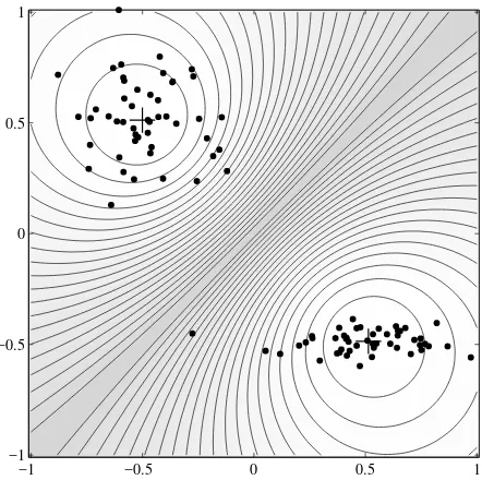
Example 4.4 Fuzzyc-means clustering. Consider a synthetic data set inR2, which contains two well-separated clusters of different shapes, as depicted in Figure 4.4. The samples in both clusters are drawn from the normal distribution. The standard devia-tion for the upper cluster is 0.2 for both axes, whereas in the lower cluster it is 0.2 for the horizontal axis and 0.05 for the vertical axis. The FCM algorithm was applied to this data set. The norm-inducing matrix was set toA=Ifor both clusters, the weight-ing exponent tom= 2, and the termination criterion toǫ = 0.01. The algorithm was initialized with a random partition matrix and converged after 4 iterations. From the membership level curves in Figure 4.4, one can see that the FCM algorithm imposes a circular shape on both clusters, even though the lower cluster is rather elongated.
−1 −0.5 0 0.5 1
1
0.5
0
−0.5
−1
Figure 4.4. The fuzzy c-means algorithm imposes a spherical shape on the clusters, re-gardless of the actual data distribution. The dots represent the data points, ‘+’ are the cluster means. Also shown are level curves of the clusters. Dark shading corresponds to membership degrees around 0.5.
to how to choose them a priori. In Section 4.4, we will see that these matrices can be adapted by using estimates of the data covariance. A partition obtained with the Gustafson–Kessel algorithm, which uses such an adaptive distance norm, is presented in Example 4.5.
✷
Initial Partition Matrix. The partition matrix is usually initialized at random, such thatU ∈ Mf c. A simple approach to obtain suchU is to initialize the cluster
centersvi at random and compute the correspondingU by (4.8a) (i.e., by using the third step of the FCM algorithm).
4.3.4 Extensions of the Fuzzy
c
-Means AlgorithmThere are several well-known extensions of the basicc-means algorithm:
Algorithms using an adaptive distance measure, such as the Gustafson–Kessel algo-rithm (Gustafson and Kessel, 1979) and the fuzzy maximum likelihood estimation algorithm (Gath and Geva, 1989).
Algorithms based on hyperplanar or functional prototypes, or prototypes defined by functions. They include the fuzzyc-varieties (Bezdek, 1981), fuzzyc-elliptotypes (Bezdek, et al., 1981), and fuzzy regression models (Hathaway and Bezdek, 1993). Algorithms that search for possibilistic partitions in the data, i.e., partitions where the constraint (4.4b) is relaxed.
In the following sections we will focus on the Gustafson–Kessel algorithm. 4.4 Gustafson–Kessel Algorithm
Gustafson and Kessel (Gustafson and Kessel, 1979) extended the standard fuzzy c-means algorithm by employing an adaptive distance norm, in order to detect clusters of different geometrical shapes in one data set. Each cluster has its own norm-inducing matrixAi, which yields the following inner-product norm:
D2ikAi = (zk −vi)TAi(zk−vi). (4.13)
The matricesAi are used as optimization variables in the c-means functional, thus
allowing each cluster to adapt the distance norm to the local topological structure of the data. The objective functional of the GK algorithm is defined by:
J(Z;U,V,{Ai}) =
c
i=1
N
k=1
(µik)mDik2Ai (4.14)
This objective function cannot be directly minimized with respect toAi, since it is linear inAi. To obtain a feasible solution,Ai must be constrained in some way. The
usual way of accomplishing this is to constrain the determinant ofAi:
Allowing the matrix Ai to vary with its determinant fixed corresponds to optimiz-ing the cluster’s shape while its volume remains constant. By usoptimiz-ing the Lagrange-multiplier method, the following expression forAiis obtained (Gustafson and Kessel,
1979):
Ai= [ρidet(Fi)]1/nF−1i , (4.16)
whereFiis thefuzzy covariance matrixof theith cluster given by
Fi= N
k=1
(µik)m(zk−vi)(zk −vi)T
N
k=1 (µik)m
. (4.17)
Note that the substitution of equations (4.16) and (4.17) into (4.13) gives a generalized squared Mahalanobis distance norm, where the covariance is weighted by the mem-bership degrees inU. The GK algorithm is given in Algorithm 4.2 and its MATLAB
Algorithm 4.2 Gustafson–Kessel (GK) algorithm.
Given the data setZ, choose the number of clusters1 < c < N, the weighting expo-nentm > 1and the termination toleranceǫ > 0and the cluster volumesρi. Initialize
the partition matrix randomly, such thatU(0)∈Mf c. Repeat forl = 1,2, . . .
Step 1: Compute cluster prototypes (means):
v(il) =
Step 2: Compute the cluster covariance matrices:
Fi=
Step 3: Compute the distances: D2ikAi = (zk−v
Step 4: Update the partition matrix: for 1≤k ≤N
4.4.1 Parameters of the Gustafson–Kessel Algorithm
cluster volumes ρi. Without any prior knowledge, ρi is simply fixed at 1 for each
cluster. A drawback of the this setting is that due to the constraint (4.15), the GK algorithm only can find clusters of approximately equal volumes.
4.4.2 Interpretation of the Cluster Covariance Matrices
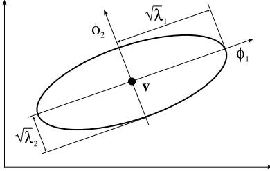
The eigenstructure of the cluster covariance matrixFiprovides information about the shape and orientation of the cluster. The ratio of the lengths of the cluster’s hyper-ellipsoid axes is given by the ratio of the square roots of the eigenvalues ofFi. The
directions of the axes are given by the eigenvectors of Fi, as shown in Figure 4.5. The GK algorithm can be used to detect clusters along linear subspaces of the data space. These clusters are represented by flat hyperellipsoids, which can be regarded as hyperplanes. The eigenvector corresponding to the smallest eigenvalue determines the normal to the hyperplane, and can be used to compute optimal local linear models from the covariance matrix.
v
√λ1
√λ2
φ2
φ1
Figure 4.5. Equation(z−v)TF−1(x−v) = 1defines a hyperellipsoid. The length of
thejth axis of this hyperellipsoid is givenby√λj and its direction is spanned byφj, where
λj andφj are thejth eigenvalue and the corresponding eigenvector of F, respectively.
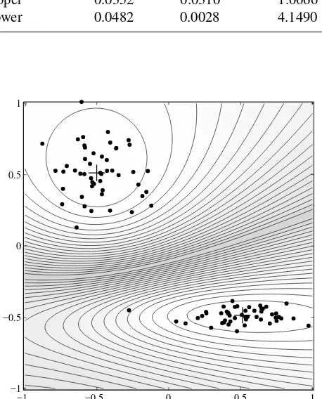
Example 4.5 Gustafson–Kessel algorithm. The GK algorithm was applied to the data set from Example 4.4, using the same initial settings as the FCM algorithm. Fig-ure 4.4 shows that the GK algorithm can adapt the distance norm to the underlying distribution of the data. One nearly circular cluster and one elongated ellipsoidal clus-ter are obtained. The shape of the clusclus-ters can be declus-termined from the eigenstructure of the resulting covariance matricesFi. The eigenvalues of the clusters are given in
Table 4.1.
One can see that the ratios given in the last column reflect quite accurately the ratio of the standard deviations in each data group (1 and 4 respectively). For the lower cluster, the unitary eigenvector corresponding toλ2,φ2 = [0.0134,0.9999]T, can be
seen as a normal to a line representing the second cluster’s direction, and it is, indeed, nearly parallel to the vertical axis.
Table 4.1. Eigenvalues of the cluster covariance matrices for clusters in Figure 4.6.
cluster λ1 λ2
√
λ1/ √
λ2
upper 0.0352 0.0310 1.0666 lower 0.0482 0.0028 4.1490
−1 −0.5 0 0.5 1
1
0.5
0
−0.5
−1
Figure 4.6. The Gustafson–Kessel algorithm can detect clusters of different shape and orientation. The points represent the data, ‘+’ are the cluster means. Also shown are level curves of the clusters. Dark shading corresponds to membership degrees around 0.5.
4.5 Summary and Concluding Remarks
Fuzzy clustering is a powerful unsupervised method for the analysis of data and con-struction of models. In this chapter, an overview of the most frequently used fuzzy clustering algorithms has been given. It has been shown that the basicc-means iter-ative scheme can be used in combination with adaptive distance measures to reveal clusters of various shapes. The choice of the important user-defined parameters, such as the number of clusters and the fuzziness parameter, has been discussed.
4.6 Problems
2. State mathematically at least two different distance norms used in fuzzy clustering. Explain the differences between them.
3. Name two fuzzy clustering algorithms and explain how they differ from each other. 4. State the fuzzyc-mean functional and explain all symbols.