ESTIMATION OF PARAMETERS OF GENERALIZED BETA OF THE SECOND KIND (GB2) DISTRIBUTION BY MAXIMUM LIKELIHOOD ESTIMATION (MLE) AND NEWTON-RAPHSON ITERATION

(1)

http://dx.doi.org/10.17654/MS105010001

Volume 105, Number 1, 2018, Pages 1-20 ISSN: 0972-0871

Received: September 19, 2017; Revised: January 17, 2018; Accepted: March 17, 2018 Keywords and phrases: generalized beta 2 (GB2) distribution, maximum likelihood estimation (MLE), Newton-Raphson.

ESTIMATION OF PARAMETERS OF GENERALIZED

BETA OF THE SECOND KIND (GB2) DISTRIBUTION BY

MAXIMUM LIKELIHOOD ESTIMATION (MLE)

AND NEWTON-RAPHSON ITERATION

Warsono, Waryoto, Mustofa Usman and Wamiliana

Department of Mathematics

University of Lampung

Indonesia

Abstract

The aim of this study is to derive the estimates of the parameters of generalized beta of the second kind (GB2) distribution by using the maximum likelihood estimation (MLE). Due to the difficulty in finding the analytical solution by MLE approach, the estimate is determined numerically by using iteration and Newton-Raphson methods. The Newton-Raphson method is used to estimate parameters, to find a confidence interval, to estimate the bias, and to estimate the variance for some difference sample size configuration viz. for n20,30,50,100 and 500. The estimation of the parameters

(2)

1. Introduction

Many papers which have discussed the distribution of income used beta distribution [1]; gamma distribution [2-5]; and Weibull model [6]. The generalized beta distribution of the second kind (GB2) is a very flexible four-parameter distribution. It is used a lot to analyze income distribution. References [7] and [8] suggested the generalized beta of the second kind (GB2) as a model for the size distribution of income and indicators of poverty. It captures the characteristics of income distribution including skewness, peakness in low-middle range, and long right hand tail. This distribution therefore provides good description of income distribution [7, 9-11]. GB2 is used in mathematical economic, in insurance company, health science and in industry. Although a large number of functional forms have been proposed, the four-parameter generalized beta of the second kind (GB2) model is now widely acknowledged to give an excellent description of income distributions, providing the goodness-of-fit with relative parsimony, while also including many other models as special or limiting cases [7, 12-15]. [16] addressed issues of time-inconsistency in top-coded US Current Population Survey earnings data by fitting GB2 distributions that account for top-coding, and derive a consistent time series of Gini coefficients from the estimates. In [17], the model of optimization of the behavior predicts that the earnings distribution has the GB2 shape.

A random variable has a distribution of generalized beta of the second kind (GB2) with parameter



a,b, p, q



if the probability density function is of the form:

 





. 0 , , , ; 0 ,

1 ,

1

 

   

 

      

  _ x a b p q

b x q

p B b

ax x

f

q p a ap

ap

(1)

Parameter b is a scale parameter, a, p and q are each shape parameter,





   

_

_

q p

q p q

p

B ,  _ _ is the beta function, and 

 

 is the gamma

(3)

   

p q a k q a k p bk

 

           

   

and exists only if ap k  aq. Tail behavior of the distribution depends on ap (lower tail) and aq (upper tail), with larger values ofareducing the density at both tails, and the relative sizes ofpandq

affecting skewness [10, 18].

The aim of this study is to estimate the parameters of the GB2 distribution by using the maximum likelihood estimation (MLE) method and then the simulation by using Software R is used to estimate the parameters for some difference sample size configuration, namely for the sample sizes: 20, 30, 50 100 and 500.

2. The Estimation

The estimation of parameters GB2 by MLE

To estimate the parameter by using the maximum likelihood estimation (MLE) method, first we define the likelihood function as follows:





 











 



    

  

       



 n

i

n

i _a p q

i ap

ap i i

b x q

p B b

x a x

f x

q p b a L

1 1

1

1 , ,

, ,

 









.

1 ,

1 1

1

    

  

    

  

      

  

 





 



n

i

q p a i n

nap

n

i

ap i n

b x q

p B b

x a

(2)

Applying the natural logarithm to equation (2) above, we have





 









  

  

 

  

  

 

    

  

    

  

      

  

 







 



n

i

q p a i n

nap

n

i

ap i n

b x q

p B b

x a

x q p b a L

1 1

1

1 ,

ln ,

(4)







 





  

 

 n

i xi nap n B p q

ap a n

1ln 1 ln ,

1 ln







_

    

  

       

 n

i

a i

b x q

p

1ln 1 , (3)

where



,



 

_

 

_

,

q p

q p q

p

B  _ _ B



p, q



is the beta function and 

 

p is the gamma function, then equation (3) can be written as:











 



  

  



n

i

i nap b n p

x ap

a n x q p b a L

1

ln ln

ln 1 ln

, , , ln

 

q n



p q



n    

 ln ln







 __

 

  

       

 n

i

a i

b x q

p

1ln 1 . (4)

Next, we set the first derivatives with respect to the parameters of

interest equal to zero as follows:

 

. 0

ln _

 

  L

The first derivative with respect toais set equal to zero,





, 0 ,

, ,

ln _

  

a

x q p b a L

 

ˆln ˆ





ln 1 0,

ln

ˆ ˆ

1 1



 

     

  

    

  

       

   



n

i

n

i

a i

i _b

x q

p a b p n x p

a n

 











 

     

     

   

 

   

 

      

            

 

 n

i

n

i a

i i a i

i

b x

b x b

x q

p b p n x p

a n

1 1 ˆ

ˆ

. 0

ˆ

1

ˆ

ln

ˆ ˆ

ln

ˆ

ln

ˆ

(5)

The first derivative with respect tobis set equal to zero,

Let

,

The first derivative with respect topis set equal to zero,

(6)

Equation (7) can be written as follows:

 







  __ 

 

  

       

    

 n

i

a i n

i i _b

x q

p n p n b n a x a

1

ˆ

1 ln 1 ˆ 0.

ˆ ˆ ˆ

ˆ

ln

ˆ

ln

ˆ ₍₈₎

The first derivative with respect toqis set equal to zero,





, 0 ,

, ,

ln _

  

p

x q p b a L

 



ˆ ˆ



ln 1 ˆ 0,

ˆ ˆ ˆ

ˆ

1

ˆ





     

  

       

 

   

 n

i

a i

b x q

p q p n q

q n

 







 __ 

 

  

       

  

 n

i

a i

b x q

p n q n

1

ˆ

. 0

ˆ

1 ln

ˆ ˆ

ˆ ₍₉₎

Equations (5), (6), (8) and (9) are very difficult to be solved by

analytical method. Thus, the Newton-Raphson method will be used to

estimate the parametersa,b,p andq. To estimate the parametersa,b,pand

qby using Newton-Raphson method, first we find the gradient vector and the first derivative vector from the logarithm function with respect toa,b,pand

qand define g

 

 as follows:

 





















.

, , , ln

        

 

        

 

  

 

  

 

q

x q p b a L

p

x q p b a L

b

x q p b a L

a

x q p b a L

g (10)

The Hessian matrix which was found from the second derivative of the

(7)

 

   L



_a__b_p qx



The iteration process by using the Newton-Raphson method is:

  





 

, function with respect to the respective parameters.

The second derivative of equation (5) with respect toais

(8)

  0.

The second derivative of equation (5) with respect tobis

(9)



The second derivative of equation (5) with respect topis





The second derivative of equation (5) with respect toqis

(10)

.

(11)







(12)

(13)







_













(14)

 









(15)





, 0 ,

, , ln

2

 



 

a q

x q p b a L



 

      

              n

i a

i i a i

b x

b x b

x

1 ˆ

ˆ

. 0

ˆ

1

ˆ

ln

ˆ

(25)





, 0 ,

, , ln

2

 



 

b q

x q p b a L









    

  

      

     

n

i a

i a i i

b x b

b x x a

1 ˆ

2

1 ˆ

. 0

ˆ

1

ˆ ˆ ˆ

(26)

The second derivative of equation (9) with respect to is





, 0 ,

, , ln

2

 



 

p q

x q p b a L



ˆ  ˆ



 0.

 p q

n (27)





, 0 ,

, , ln

2

 



 

q q

x q p b a L

 

ˆ  



ˆ  ˆ



 0.

 q n p q

n (28)

3. Simulation Result and Discussion

To find the Hessian matrix, we substitute the result from the second derivative of logarithm function with respect to the respective parameters

(16)

values for the respective parameters as a  2; b 1, 2; p 15 and .

75 , 0



q In generating the sample, we use the sample sizes forn equals to

20, 30, 50, 100 and 500 and the number of iterations 100 for respective sample sizes. From the simulation, we calculate the mean, bias, variances and confidence interval (CI) for respective sample sizes n  20, 30, 50, 100 and 500.

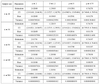
Table 1. Estimation value, confidence interval (CI), bias, and variances of generalized beta II (GB2) for the parameters a  2; b 1.2; p 15 and

, 75 . 0



q sample sizes n  20, 30,50,100 and 500

Sample size Parameters a2 b1.2 p15 q0.75 Estimation 2.02889 1.23003 15.02581 0.76278

CI [2.01148; 2.04630] [1.21727; 1.24279] [14.99674; 15.05488] [0.74040; 0.78516] Bias 0.02889 0.03003 0.02581 0.01278 20

 n

Variance 0.0000789261 0.0000423958 0.0002199300 0.0001304063 Estimation 2.02609 1.22833 15.02016 0.76178

CI [2.01521; 2.03697] [1.21715; 1.23951] [15.01211; 15.02822] [0.75515; 0.76841] Bias 0.02609 0.02833 0.02016 0.01178 30

 n

CI [2.01428; 2.02154] [1.22457; 1.22747] [15.01527; 15.02033] [0.75810; 0.76403] Bias 0.01791 0.02602 0.01780 0.01107 50

 n

CI [2.00914; 2.01261] [1.20208; 1.20407] [15.00651; 15.00743] [0.75003; 0.75075] Bias 0.01088 0.00308 0.00697 0.00039 100

 n

CI [2.00990; 2.01008] [1.20281; 1.20321] [15.00388; 15.00413] [0.75019; 0.75021] Bias 0.00999 0.00301 0.00400 0.00020 500

 n

Variance 0.0000000021 0.0000000102 0.0000000039 0.0000000001

From the results of the simulation given in Table 1, we can conclude that

when the sample size increases, the estimation values and the real values are

close. Further, when the sample size is larger, the confidence interval will be

(17)

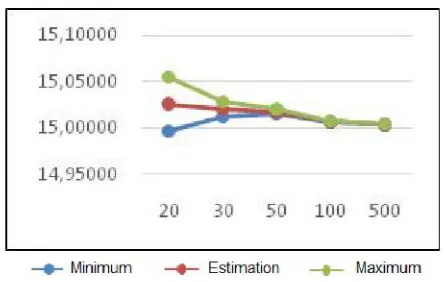
Figures 1 to 6 describe the estimation of parameters and its confidence

intervals, bias and variances.

Figure 1. The graph of theaestimation and its confident interval (CI).

Figure 2. The graph of thebestimation and its confident interval (CI).

(18)

Figure 4. The graph of theqestimation and its confidence interval (CI).

Figure 5. The graph of bias for the parametersa,b,pandqof the (GB2).

(19)

4. Conclusion

The estimation of parameters of generalized beta of the second

kind (GB2) uses maximum likelihood estimation (MLE) method. Then the

estimation is continued by iteration and Newton-Raphson methods. The

results show that the estimation of the parameters a, b, p and q attains the values close to the real value of the parameters, if the size of the sample

increases. The larger the sample size, the narrower the confidence interval is.

The larger the sample size is, the smaller the bias and the variance are.

Acknowledgement

The authors thank the anonymous referees for their valuable suggestions

leading to the improvement of the manuscript.

References

[1] L. C. Thurow, Analyzing the American income distribution, paper and proceedings, American Economics Association 60 (1970), 261-269.

[2] C. Taille, Lorenz ordering within the generalized gamma family of income distributions, Statistical Distributions in Scientific Work, C. Taille, G. P. Patil and B. Balderssari, eds., Reidel, Boston, Vol. 6, 1981, pp. 182-192.

[3] J. B. McDonald and B. C. Jensen, An analysis of estimators of alternative measures of income inequality associated with the gamma distribution function, J. Amer. Statist. Assoc. 74 (1979), 856-860.

[4] A. B. Salem and T. D. Mount, A convenient descriptive model of income distribution: the gamma density, Econometrica 44 (1974), 963-970.

[5] S. K. Singh and G. S. Maddala, A function for the size distribution of income, Econometrica 44 (1976), 963-970.

[6] C. P. A. Bartels and H. Van Metele, Alternative Probability Density Functions of Income, Vrije University Amsterdam: Research Memorandum 29, 1975.

(20)

[8] M. Graf and D. Nedyalkova, Modeling of income and indicators of poverty and social exclusion using the generalized beta distribution of the second kind, Review of Income and Wealth 60 (2014), 821-842. Doi: 10.1111/roiw.12031. [9] Stephen P. Jenkins, Inequality and the GB2 income distribution, ISER, University

of Essex, DIW Berlin and IZA Discussion Paper No. 2831, 2007.

[10] Stephen P. Jenkins, Distributionally-sensitive inequality indices and the GB2 income distribution, Review of Income and Wealth Series 55(2) (2009), 392-398. [11] C. Kleiber, On the Lorenz order within parametric families of income

distributions, Sankhya 61 (1999), 314-317.

[12] R. F. Bordley, J. B. McDonald and A. Mantrala, Something new, something old: parametric models for the size distribution of income, Journal of Income Distribution 6 (1996), 91-103.

[13] K. Brachmann, A. Stich and M. Trede, Evaluating parametric income distribution models, Allg. Stat. Arch. 80 (1996), 285-298.

[14] J. B. Butler and J. B. McDonald, Using incomplete moments to measure inequality, J. Econometrics 42 (1989), 109-119.

[15] J. B. McDonald and Y. J. Xu, A generalization of the beta distribution with applications, J. Econometrics 66 (1995), 133-152.

[16] S. Feng, R. V. Burkhauser and J. S. Butler, Levels and long-term trends in earnings inequality: overcoming current population survey censoring problems using the GB2 distribution, J. Bus. Econom. Statist. 24 (2006), 57-62.

[17] S. C. Parker, The generalized beta as a model for the distribution of earnings, Econom. Lett. 62 (1999), 197-200.

[18] C. Kleiber and S. Kotz, Statistical Size Distributions in Economics and Actuarial Sciences, Hoboken, Wiley-Interscience, NJ, USA, 2003.