Oorschot, and S. Vanstone, CRC Press, 1996.
For further information, see
www.cacr.math.uwaterloo.ca/hac
CRC Press has granted the following specific permissions for the electronic version of this
book:
Permission is granted to retrieve, print and store a single copy of this chapter for
personal use. This permission does not extend to binding multiple chapters of
the book, photocopying or producing copies for other than personal use of the
person creating the copy, or making electronic copies available for retrieval by
others without prior permission in writing from CRC Press.
Except where over-ridden by the specific permission above, the standard copyright notice
from CRC Press applies to this electronic version:
Neither this book nor any part may be reproduced or transmitted in any form or
by any means, electronic or mechanical, including photocopying, microfilming,
and recording, or by any information storage or retrieval system, without prior
permission in writing from the publisher.
The consent of CRC Press does not extend to copying for general distribution,
for promotion, for creating new works, or for resale. Specific permission must be
obtained in writing from CRC Press for such copying.
c
Stream Ciphers
Contents in Brief
6.1 Introduction. . . 191
6.2 Feedback shift registers. . . 195
6.3 Stream ciphers based on LFSRs . . . 203
6.4 Other stream ciphers . . . 212
6.5 Notes and further references . . . 216
6.1 Introduction
Stream ciphersare an important class of encryption algorithms. They encrypt individual characters (usually binary digits) of a plaintext message one at a time, using an encryp-tion transformaencryp-tion which varies with time. By contrast,block ciphers(Chapter 7) tend to simultaneously encrypt groups of characters of a plaintext message using a fixed encryp-tion transformaencryp-tion. Stream ciphers are generally faster than block ciphers in hardware, and have less complex hardware circuitry. They are also more appropriate, and in some cases mandatory (e.g., in some telecommunications applications), when buffering is lim-ited or when characters must be individually processed as they are received. Because they have limited or no error propagation, stream ciphers may also be advantageous in situations where transmission errors are highly probable.
There is a vast body of theoretical knowledge on stream ciphers, and various design principles for stream ciphers have been proposed and extensively analyzed. However, there are relatively few fully-specified stream cipher algorithms in the open literature. This un-fortunate state of affairs can partially be explained by the fact that most stream ciphers used in practice tend to be proprietary and confidential. By contrast, numerous concrete block cipher proposals have been published, some of which have been standardized or placed in the public domain. Nevertheless, because of their significant advantages, stream ciphers are widely used today, and one can expect increasingly more concrete proposals in the coming years.
Chapter outline
a nonlinear combining function on the outputs of several LFSRs (§6.3.1), using a nonlin-ear filtering function on the contents of a single LFSR (§6.3.2), and using the output of one (or more) LFSRs to control the clock of one (or more) other LFSRs (§6.3.3). Two concrete proposals for clock-controlled generators, the alternating step generator and the shrinking generator are presented in§6.3.3.§6.4 presents a stream cipher not based on LFSRs, namely SEAL.§6.5 concludes with references and further chapter notes.
6.1.1 Classification
Stream ciphers can be either symmetric-key or public-key. The focus of this chapter is symmetric-key stream ciphers; the Blum-Goldwasser probabilistic public-key encryption scheme (§8.7.2) is an example of a public-key stream cipher.
6.1 Note (block vs. stream ciphers) Block ciphers process plaintext in relatively large blocks (e.g.,n ≥ 64bits). The same function is used to encrypt successive blocks; thus (pure) block ciphers arememoryless. In contrast, stream ciphers process plaintext in blocks as small as a single bit, and the encryption function may vary as plaintext is processed; thus stream ciphers are said to have memory. They are sometimes calledstate cipherssince encryption depends on not only the key and plaintext, but also on the current state. This distinction between block and stream ciphers is not definitive (see Remark 7.25); adding a small amount of memory to a block cipher (as in the CBC mode) results in a stream cipher with large blocks.
(i) The one-time pad
Recall (Definition 1.39) that aVernam cipherover the binary alphabet is defined by
ci=mi⊕ki fori= 1,2,3. . . ,
wherem1, m2, m3, . . . are the plaintext digits,k1, k2, k3, . . . (thekeystream) are the key
digits,c1, c2, c3, . . . are the ciphertext digits, and⊕is the XOR function (bitwise addition
modulo2). Decryption is defined bymi = ci⊕ki. If the keystream digits are generated
independently and randomly, the Vernam cipher is called aone-time pad, and is uncondi-tionally secure (§1.13.3(i)) against a ciphertext-only attack. More precisely, ifM,C, and Kare random variables respectively denoting the plaintext, ciphertext, and secret key, and ifH()denotes the entropy function (Definition 2.39), thenH(M|C) = H(M). Equiva-lently,I(M;C) = 0(see Definition 2.45): the ciphertext contributes no information about the plaintext.
Shannon proved that a necessary condition for a symmetric-key encryption scheme to be unconditionally secure is thatH(K) ≥ H(M). That is, the uncertainty of the secret key must be at least as great as the uncertainty of the plaintext. If the key has bitlengthk, and the key bits are chosen randomly and independently, thenH(K) =k, and Shannon’s necessary condition for unconditional security becomesk ≥H(M). The one-time pad is unconditionally secure regardless of the statistical distribution of the plaintext, and is op-timal in the sense that its key is the smallest possible among all symmetric-key encryption schemes having this property.
Stream ciphers are commonly classified as beingsynchronousorself-synchronizing.
(ii) Synchronous stream ciphers
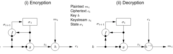
6.2 Definition Asynchronousstream cipher is one in which the keystream is generated inde-pendently of the plaintext message and of the ciphertext.
The encryption process of a synchronous stream cipher can be described by the equations
σi+1 = f(σi, k),
zi = g(σi, k),
ci = h(zi, mi),
whereσ0 is theinitial stateand may be determined from the keyk,f is thenext-state
function,gis the function which produces thekeystreamzi, andhis theoutput function
which combines the keystream and plaintextmi to produce ciphertextci. The encryption
and decryption processes are depicted in Figure 6.1. The OFB mode of a block cipher (see §7.2.2(iv)) is an example of a synchronous stream cipher.
zi
Figure 6.1:General model of a synchronous stream cipher.
6.3 Note (properties of synchronous stream ciphers)
(i) synchronization requirements. In a synchronous stream cipher, both the sender and receiver must besynchronized– using the same key and operating at the same posi-tion (state) within that key – to allow for proper decrypposi-tion. If synchronizaposi-tion is lost due to ciphertext digits being inserted or deleted during transmission, then decryption fails and can only be restored through additional techniques for re-synchronization. Techniques for re-synchronization include re-initialization, placing special markers at regular intervals in the ciphertext, or, if the plaintext contains enough redundancy, trying all possible keystream offsets.
(ii) no error propagation. A ciphertext digit that is modified (but not deleted) during transmission does not affect the decryption of other ciphertext digits.
(iii) active attacks. As a consequence of property (i), the insertion, deletion, or replay of ciphertext digits by an active adversary causes immediate loss of synchronization, and hence might possibly be detected by the decryptor. As a consequence of property (ii), an active adversary might possibly be able to make changes to selected ciphertext digits, and know exactly what affect these changes have on the plaintext. This illus-trates that additional mechanisms must be employed in order to provide data origin authentication and data integrity guarantees (see§9.5.4).
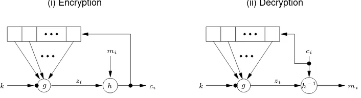
6.4 Definition Abinary additive stream cipheris a synchronous stream cipher in which the keystream, plaintext, and ciphertext digits are binary digits, and the output functionhis the XOR function.
Binary additive stream ciphers are depicted in Figure 6.2. Referring to Figure 6.2, the
keystream generatoris composed of the next-state functionf and the functiong(see Fig-ure 6.1), and is also known as therunning key generator.
Generator Keystream
mi
zi
ci
mi
ci
Plaintextmi
Ciphertextci Keyk Keystreamzi
zi
k
k Keystream
Generator
(ii) Decryption (i) Encryption
Figure 6.2:General model of a binary additive stream cipher.
(iii) Self-synchronizing stream ciphers
6.5 Definition Aself-synchronizingorasynchronousstream cipher is one in which the key-stream is generated as a function of the key and a fixed number of previous ciphertext digits.
The encryption function of a self-synchronizing stream cipher can be described by the equations
σi = (ci−t, ci−t+1, . . . , ci−1),
zi = g(σi, k),
ci = h(zi, mi),
whereσ0 = (c−t, c−t+1, . . . , c−1)is the (non-secret)initial state,kis thekey,g is the
function which produces thekeystreamzi, andhis theoutput functionwhich combines
the keystream and plaintextmi to produce ciphertextci. The encryption and decryption
processes are depicted in Figure 6.3. The most common presently-used self-synchronizing stream ciphers are based on block ciphers in 1-bit cipher feedback mode (see§7.2.2(iii)).
h
k zi ci
(i) Encryption
g
k zi mi
(ii) Decryption
g h−1
ci
mi
6.6 Note (properties of self-synchronizing stream ciphers)
(i) self-synchronization.Self-synchronization is possible if ciphertext digits are deleted or inserted, because the decryption mapping depends only on a fixed number of pre-ceding ciphertext characters. Such ciphers are capable of re-establishing proper de-cryption automatically after loss of synchronization, with only a fixed number of plaintext characters unrecoverable.
(ii) limited error propagation.Suppose that the state of a self-synchronization stream ci-pher depends ontprevious ciphertext digits. If a single ciphertext digit is modified (or even deleted or inserted) during transmission, then decryption of up tot subse-quent ciphertext digits may be incorrect, after which correct decryption resumes. (iii) active attacks. Property (ii) implies that any modification of ciphertext digits by an
active adversary causes several other ciphertext digits to be decrypted incorrectly, thereby improving (compared to synchronous stream ciphers) the likelihood of being detected by the decryptor. As a consequence of property (i), it is more difficult (than for synchronous stream ciphers) to detect insertion, deletion, or replay of ciphertext digits by an active adversary. This illustrates that additional mechanisms must be employed in order to provide data origin authentication and data integrity guarantees (see§9.5.4).
(iv) diffusion of plaintext statistics. Since each plaintext digit influences the entire fol-lowing ciphertext, the statistical properties of the plaintext are dispersed through the ciphertext. Hence, self-synchronizing stream ciphers may be more resistant than syn-chronous stream ciphers against attacks based on plaintext redundancy.
6.2 Feedback shift registers
Feedback shift registers, in particular linear feedback shift registers, are the basic compo-nents of many keystream generators.§6.2.1 introduces linear feedback shift registers. The linear complexity of binary sequences is studied in§6.2.2, while the Berlekamp-Massey al-gorithm for computing it is presented in§6.2.3. Finally, nonlinear feedback shift registers are discussed in§6.2.4.
6.2.1 Linear feedback shift registers
Linear feedback shift registers (LFSRs) are used in many of the keystream generators that have been proposed in the literature. There are several reasons for this:
1. LFSRs are well-suited to hardware implementation; 2. they can produce sequences of large period (Fact 6.12);
3. they can produce sequences with good statistical properties (Fact 6.14); and 4. because of their structure, they can be readily analyzed using algebraic techniques.
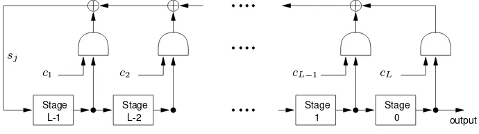
6.7 Definition Alinear feedback shift register(LFSR) of lengthLconsists ofLstages(or
delay elements) numbered0,1, . . . , L−1, each capable of storing one bit and having one input and one output; and a clock which controls the movement of data. During each unit of time the following operations are performed:
(ii) the content of stageiis moved to stagei−1for eachi,1≤i≤L−1; and (iii) the new content of stageL−1is thefeedback bitsj which is calculated by adding
together modulo2the previous contents of a fixed subset of stages0,1, . . . , L−1.
Figure 6.4 depicts an LFSR. Referring to the figure, eachciis either0or1; the closed
semi-circles are AND gates; and the feedback bitsjis the modulo2sum of the contents of
those stagesi,0≤i≤L−1, for whichcL−i= 1.
Figure 6.4:A linear feedback shift register (LFSR) of lengthL.
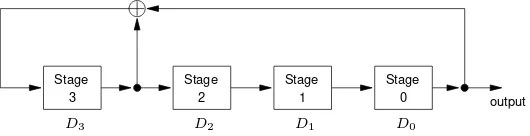
6.8 Definition The LFSR of Figure 6.4 is denotedL, C(D), whereC(D) = 1 +c1D+
Stage 3
Stage 1
Stage Stage
2 0 output
D3 D2 D1 D0
Figure 6.5:The LFSR4,1 +D+D4
of Example 6.10.
6.11 Fact Every output sequence (i.e., for all possible initial states) of an LFSRL, C(D)is periodic if and only if the connection polynomialC(D)has degreeL.
If an LFSRL, C(D)issingular(i.e.,C(D)has degree less thanL), then not all out-put sequences are periodic. However, the outout-put sequences areultimately periodic; that is, the sequences obtained by ignoring a certain finite number of terms at the beginning are periodic. For the remainder of this chapter, it will be assumed that all LFSRs are non-singular. Fact 6.12 determines the periods of the output sequences of some special types of non-singular LFSRs.
6.12 Fact (periods of LFSR output sequences) LetC(D)∈Z2[D]be a connection polynomial
of degreeL.
(i) IfC(D)is irreducible overZ2(see Definition 2.190), then each of the2L−1
non-zero initial states of the non-singular LFSRL, C(D)produces an output sequence with period equal to the least positive integerN such thatC(D)divides1 +DNin Z2[D]. (Note: it is always the case that thisNis a divisor of2L−1.)
(ii) IfC(D)is a primitive polynomial (see Definition 2.228), then each of the2L−1
non-zero initial states of the non-singular LFSRL, C(D)produces an output sequence with maximum possible period2L−1.
A method for generating primitive polynomials overZ2uniformly at random is given
in Algorithm 4.78. Table 4.8 lists a primitive polynomial of degreemoverZ2for eachm,
1≤m≤229. Fact 6.12(ii) motivates the following definition.
6.13 Definition IfC(D) ∈ Z2[D]is a primitive polynomial of degreeL, thenL, C(D)is
called amaximum-lengthLFSR. The output of a maximum-length LFSR with non-zero ini-tial state is called anm-sequence.
Fact 6.14 demonstrates that the output sequences of maximum-length LFSRs have good statistical properties.
6.14 Fact (statistical properties ofm-sequences) Letsbe anm-sequence that is generated by a maximum-length LFSR of lengthL.
(i) Letkbe an integer,1≤k ≤ L, and letsbe any subsequence ofsof length2L+
k−2. Then each non-zero sequence of lengthkappears exactly2L−k times as a
subsequence ofs. Furthermore, the zero sequence of lengthkappears exactly2L−k−
1times as a subsequence ofs. In other words, the distribution of patterns having fixed length of at mostLis almost uniform.
6.15 Example (m-sequence) SinceC(D) = 1 +D+D4is a primitive polynomial overZ 2,
the LFSR4,1 +D+D4is a maximum-length LFSR. Hence, the output sequence of this
LFSR is anm-sequence of maximum possible periodN = 24−1 = 15(cf. Example 6.10).
Example 5.30 verifies that this output sequence satisfies Golomb’s randomness properties.
6.2.2 Linear complexity
This subsection summarizes selected results about the linear complexity of sequences. All sequences are assumed to be binary sequences. Notation: sdenotes an infinite sequence whose terms ares0, s1, s2, . . .;sn denotes a finite sequence of lengthnwhose terms are
s0, s1, . . . , sn−1(see Definition 5.24).
6.16 Definition An LFSR is said togeneratea sequencesif there is some initial state for which the output sequence of the LFSR iss. Similarly, an LFSR is said togeneratea finite se-quencesnif there is some initial state for which the output sequence of the LFSR hassn
as its firstnterms.
6.17 Definition Thelinear complexityof an infinite binary sequences, denotedL(s), is defined as follows:
(i) ifsis the zero sequences= 0,0,0, . . ., thenL(s) = 0; (ii) if no LFSR generatess, thenL(s) =∞;
(iii) otherwise,L(s)is the length of the shortest LFSR that generatess.
6.18 Definition Thelinear complexityof a finite binary sequencesn, denotedL(sn), is the
length of the shortest LFSR that generates a sequence havingsnas its firstnterms.
Facts 6.19 – 6.22 summarize some basic results about linear complexity.
6.19 Fact (properties of linear complexity) Letsandtbe binary sequences.
(i) For anyn≥1, the linear complexity of the subsequencesnsatisfies0≤L(sn)≤n.
of the2L−1non-zero initial states of the non-singular LFSRL, C(D)produces an output
sequence with linear complexityL.
6.21 Fact (expectation and variance of the linear complexity of a random sequence) Letsnbe
chosen uniformly at random from the set of all binary sequences of lengthn, and letL(sn)
be the linear complexity ofsn. LetB(n)denote the parity function:B(n) = 0ifnis even;
B(n) = 1ifnis odd.
(i) The expected linear complexity ofsnis
(ii) The variance of the linear complexity ofsnisVar(L(sn)) =
6.22 Fact (expectation of the linear complexity of a random periodic sequence) Letsnbe
cho-sen uniformly at random from the set of all binary sequences of lengthn, wheren= 2tfor
some fixedt ≥ 1, and letsbe then-periodic infinite sequence obtained by repeating the sequencesn. Then the expected linear complexity ofsisE(L(sn)) =n−1 + 2−n.
The linear complexity profile of a binary sequence is introduced next.
6.23 Definition Lets =s0, s1, . . . be a binary sequence, and letLN denote the linear
com-plexity of the subsequencesN = s
0, s1, . . . , sN−1,N ≥ 0. The sequenceL1, L2, . . .
is called thelinear complexity profile ofs. Similarly, ifsn = s
0, s1, . . . , sn−1is a finite
binary sequence, the sequenceL1, L2, . . . , Lnis called thelinear complexity profile ofsn.
The linear complexity profile of a sequence can be computed using the Berlekamp-Massey algorithm (Algorithm 6.30); see also Note 6.31. The following properties of the linear complexity profile can be deduced from Fact 6.29.
6.24 Fact (properties of linear complexity profile) LetL1, L2, . . . be the linear complexity
pro-file of a sequences=s0, s1, . . ..
(i) Ifj > i, thenLj≥Li.
(ii) LN+1> LNis possible only ifLN≤N/2.
(iii) IfLN+1> LN, thenLN+1+LN=N+ 1.
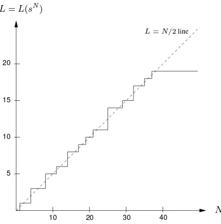
The linear complexity profile of a sequencescan be graphed by plotting the points
(N, LN),N ≥ 1, in theN ×Lplane and joining successive points by a horizontal line
followed by a vertical line, if necessary (see Figure 6.6). Fact 6.24 can then be interpreted as saying that the graph of a linear complexity profile is non-decreasing. Moreover, a (vertical) jump in the graph can only occur from below the lineL=N/2; if a jump occurs, then it is symmetric about this line. Fact 6.25 shows that the expected linear complexity of a random sequence should closely follow the lineL=N/2.
6.25 Fact (expected linear complexity profile of a random sequence) Lets =s0, s1, . . . be a
random sequence, and letLNbe the linear complexity of the subsequencesN=s0, s1, . . . ,
sN−1for eachN ≥ 1. For any fixed indexN ≥ 1, the expected smallestj for which
LN+j> LNis2ifLN ≤N/2, or2 + 2LN−N ifLN > N/2. Moreover, the expected
increase in linear complexity is2ifLN ≥N/2, orN−2LN+ 2ifLN< N/2.
6.26 Example (linear complexity profile) Consider the20-periodic sequenceswith cycle
s20 = 1,0,0,1,0,0,1,1,1,1,0,0,0,1,0,0,1,1,1,0.
The linear complexity profile ofsis1,1,1,3,3,3,3,5,5,5,6,6,6,8,8,8,9,9,10,10,11,
11,11,11,14,14,14,14,15,15,15,17,17,17,18,18,19,19,19,19, . . .. Figure 6.6 shows
10 30 20
15
10
5
20 40
L=L(sN
)
N
L=N/2line
Figure 6.6:Linear complexity profile of the20-periodic sequence of Example 6.26.
As is the case with all statistical tests for randomness (cf.§5.4), the condition that a se-quenceshave a linear complexity profile that closely resembles that of a random sequence isnecessarybut notsufficientforsto be considered random. This point is illustrated in the following example.
6.27 Example (limitations of the linear complexity profile) The linear complexity profile of the sequencesdefined as
si =
1, ifi= 2j−1for somej≥0,
0, otherwise,
follows the lineL = N/2as closely as possible. That is,L(sN) =⌊(N + 1)/2⌋for all
N≥1. However, the sequencesis clearly non-random.
6.2.3 Berlekamp-Massey algorithm
The Berlekamp-Massey algorithm (Algorithm 6.30) is an efficient algorithm for determin-ing the linear complexity of a finite binary sequencesnof lengthn(see Definition 6.18).
The algorithm takesniterations, with theNth iteration computing the linear complexity of the subsequencesN consisting of the firstN terms ofsn. The theoretical basis for the
algorithm is Fact 6.29.
6.28 Definition Consider the finite binary sequencesN+1=s
0, s1, . . . , sN−1, sN. ForC(D)
= 1 +c1D+· · ·+cLDL, letL, C(D)be an LFSR that generates the subsequencesN =
s0, s1, . . . , sN−1. Thenext discrepancydNis the difference betweensNand the(N+1)st
term generated by the LFSR:dN = (sN+iL=1cisN−i) mod 2.
6.29 Fact LetsN = s0, s1, . . . , sN−1be a finite binary sequence of linear complexityL =
(i) The LFSRL, C(D)also generatessN+1=s
0, s1, . . . , sN−1, sNif and only if the
next discrepancydNis equal to 0.
(ii) IfdN = 0, thenL(sN+1) =L.
(iii) SupposedN = 1. Letmthe largest integer< N such thatL(sm)< L(sN), and let
L(sm), B(D)be an LFSR of lengthL(sm)which generatessm. ThenL′, C′(D) is an LFSR of smallest length which generatessN+1, where
L′=
L, ifL > N/2, N+ 1−L, ifL≤N/2,
andC′(D) =C(D) +B(D)·DN−m.
6.30 AlgorithmBerlekamp-Massey algorithm
INPUT: a binary sequencesn =s
0, s1, s2, . . . , sn−1of lengthn.
OUTPUT: the linear complexityL(sn)ofsn,0≤L(sn)≤n.
1. Initialization.C(D)←1, L←0, m← −1, B(D)←1, N←0. 2. While(N < n)do the following:
2.1 Compute the next discrepancyd.d←(sN+iL=1cisN−i) mod 2.
2.2 Ifd= 1then do the following:
T(D)←C(D), C(D)←C(D) +B(D)·DN−m.
IfL≤N/2thenL←N+ 1−L, m←N, B(D)←T(D). 2.3 N←N+ 1.
3. Return(L).
6.31 Note (intermediate results in Berlekamp-Massey algorithm) At the end of each iteration of step 2,L, C(D)is an LFSR of smallest length which generatessN. Hence,
Algo-rithm 6.30 can also be used to compute the linear complexity profile (Definition 6.23) of a finite sequence.
6.32 Fact The running time of the Berlekamp-Massey algorithm (Algorithm 6.30) for deter-mining the linear complexity of a binary sequence of bitlengthnisO(n2)bit operations.
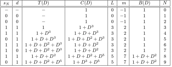
6.33 Example (Berlekamp-Massey algorithm) Table 6.1 shows the steps of Algorithm 6.30 for computing the linear complexity of the binary sequencesn= 0,0,1,1,0,1,1,1,0of length
n= 9. This sequence is found to have linear complexity5, and an LFSR which generates
it is5,1 +D3+D5.
6.34 Fact Letsnbe a finite binary sequence of lengthn, and let the linear complexity ofsnbe
L. Then there is a unique LFSR of lengthLwhich generatessnif and only ifL≤ n
2.
An important consequence of Fact 6.34 and Fact 6.24(iii) is the following.
sN d T(D) C(D) L m B(D) N
− − − 1 0 −1 1 0
0 0 − 1 0 −1 1 1
0 0 − 1 0 −1 1 2
1 1 1 1 +D3 3 2 1 3
1 1 1 +D3 1 +D+D3 3 2 1 4
0 1 1 +D+D3 1 +D+D2+D3 3 2 1 5
1 1 1 +D+D2+D3 1 +D+D2 3 2 1 6
1 0 1 +D+D2+D3 1 +D+D2 3 2 1 7
1 1 1 +D+D2 1 +D+D2+D5 5 7 1 +D+D2 8
0 1 1 +D+D2+D5 1 +D3+D5 5 7 1 +D+D2 9
Table 6.1:Steps of the Berlekamp-Massey algorithm of Example 6.33.
6.2.4 Nonlinear feedback shift registers
This subsection summarizes selected results about nonlinear feedback shift registers. A function withnbinary inputs and one binary output is called aBoolean functionofn vari-ables; there are22n different Boolean functions ofnvariables.
6.36 Definition A (general)feedback shift register(FSR) of lengthLconsists ofLstages(or
delay elements) numbered0,1, . . . , L−1, each capable of storing one bit and having one input and one output, and a clock which controls the movement of data. During each unit of time the following operations are performed:
(i) the content of stage0is output and forms part of theoutput sequence; (ii) the content of stageiis moved to stagei−1for eachi,1≤i≤L−1; and (iii) the new content of stageL−1is thefeedback bitsj = f(sj−1, sj−2, . . . , sj−L),
where thefeedback functionfis a Boolean function andsj−iis the previous content
of stageL−i,1≤i≤L.
If the initial content of stageiissi∈ {0,1}for each0≤i≤L−1, then[sL−1, . . . , s1, s0]
is called theinitial stateof the FSR.
Figure 6.7 depicts an FSR. Note that if the feedback functionfis a linear function, then the FSR is an LFSR (Definition 6.7). Otherwise, the FSR is called anonlinearFSR.
Stage
sj
Stage
L-1 L-2 1 0
Stage Stage
sj−L+1
sj−1 sj−2 sj−L
f(sj−1, sj−2, . . . , sj−L)
output
Figure 6.7:A feedback shift register (FSR) of lengthL.
6.37 Fact If the initial state of the FSR in Figure 6.7 is[sL−1, . . . , s1, s0], then the output
se-quences=s0, s1, s2, . . . is uniquely determined by the following recursion:
6.38 Definition An FSR is said to benon-singularif and only if every output sequence of the FSR (i.e., for all possible initial states) is periodic.
6.39 Fact An FSR with feedback functionf(sj−1, sj−2, . . . , sj−L)is non-singular if and only
iff is of the formf =sj−L⊕g(sj−1, sj−2, . . . , sj−L+1)for some Boolean functiong.
The period of the output sequence of a non-singular FSR of lengthLis at most2L.
6.40 Definition If the period of the output sequence (for any initial state) of a non-singular FSR of lengthLis2L, then the FSR is called ade Bruijn FSR, and the output sequence is called
ade Bruijn sequence.
6.41 Example (de Bruijn sequence) Consider the FSR of length3with nonlinear feedback functionf(x1, x2, x3) = 1⊕x2⊕x3⊕x1x2. The following tables show the contents of the
3stages of the FSR at the end of each unit of timetwhen the initial state is[0,0,0].
t Stage 2 Stage 1 Stage 0
0 0 0 0
1 1 0 0
2 1 1 0
3 1 1 1
t Stage 2 Stage 1 Stage 0
4 0 1 1
5 1 0 1
6 0 1 0
7 0 0 1
The output sequence is the de Bruijn sequence with cycle0,0,0,1,1,1,0,1. Fact 6.42 demonstrates that the output sequence of de Bruijn FSRs have good statistical properties (compare with Fact 6.14(i)).
6.42 Fact (statistical properties of de Bruijn sequences) Letsbe a de Bruijn sequence that is generated by a de Bruijn FSR of lengthL. Letkbe an integer,1≤k≤L, and letsbe any subsequence ofsof length2L+k−1. Then each sequence of lengthkappears exactly
2L−ktimes as a subsequence ofs. In other words, the distribution of patterns having fixed
length of at mostLis uniform.
6.43 Note (converting a maximum-length LFSR to a de Bruijn FSR) LetR1be a
maximum-length LFSR of maximum-lengthLwith (linear) feedback functionf(sj−1, sj−2, . . . , sj−L). Then
the FSRR2with feedback functiong(sj−1, sj−2, . . . , sj−L) =f⊕sj−1sj−2· · ·sj−L+1
is a de Bruijn FSR. Here,sidenotes the complement ofsi. The output sequence ofR2is
obtained from that ofR1by simply adding a0to the end of each subsequence ofL−1 0’s
occurring in the output sequence ofR1.
6.3 Stream ciphers based on LFSRs
(Algorithm 6.30) from any (short) subsequencetofshaving length at leastn = 2L(cf. Fact 6.35). Having determinedC(D), the LFSRL, C(D)can then be initialized with any substring ofthaving lengthL, and used to generate the remainder of the sequences. An adversary may obtain the required subsequencetofsby mounting a known or chosen-plaintext attack (§1.13.1) on the stream cipher: if the adversary knows the chosen-plaintext subse-quencem1, m2, . . . , mncorresponding to a ciphertext sequencec1, c2, . . . , cn, the
corre-sponding keystream bits are obtained asmi⊕ci,1≤i≤n.
6.44 Note (use of LFSRs in keystream generators) Since a well-designed system should be se-cure against known-plaintext attacks, an LFSR should never be used by itself as a keystream generator. Nevertheless, LFSRs are desirable because of their very low implementation costs. Three general methodologies for destroying the linearity properties of LFSRs are discussed in this section:
(i) using a nonlinear combining function on the outputs of several LFSRs (§6.3.1); (ii) using a nonlinear filtering function on the contents of a single LFSR (§6.3.2); and (iii) using the output of one (or more) LFSRs to control the clock of one (or more) other
LFSRs (§6.3.3).
Desirable properties of LFSR-based keystream generators
For essentially all possible secret keys, the output sequence of an LFSR-based keystream generator should have the following properties:
1. large period;
2. large linear complexity; and
3. good statistical properties (e.g., as described in Fact 6.14).
It is emphasized that these properties are onlynecessaryconditions for a keystream gen-erator to be considered cryptographically secure. Since mathematical proofs of security of such generators are not known, such generators can only be deemedcomputationally secure
(§1.13.3(iv)) after having withstood sufficient public scrutiny.
6.45 Note (connection polynomial) Since a desirable property of a keystream generator is that its output sequences have large periods, component LFSRs should always be chosen to be maximum-length LFSRs, i.e., the LFSRs should be of the formL, C(D)whereC(D)∈
Z2[D]is a primitive polynomial of degreeL(see Definition 6.13 and Fact 6.12(ii)).
6.46 Note (known vs. secret connection polynomial) The LFSRs in an LFSR-based keystream generator may haveknownorsecretconnection polynomials. For known connections, the secret key generally consists of the initial contents of the component LFSRs. For secret connections, the secret key for the keystream generator generally consists of both the initial contents and the connections.
For LFSRs of lengthLwith secret connections, the connection polynomials should be selected uniformly at random from the set of all primitive polynomials of degreeLoverZ2.
6.47 Note (sparse vs. dense connection polynomial) For implementation purposes, it is advan-tageous to choose an LFSR that issparse; i.e., only a few of the coefficients of the con-nection polynomial are non-zero. Then only a small number of concon-nections must be made between the stages of the LFSR in order to compute the feedback bit. For example, the con-nection polynomial might be chosen to be a primitive trinomial (cf. Table 4.8). However, in some LFSR-based keystream generators, special attacks can be mounted if sparse connec-tion polynomials are used. Hence, it is generally recommended not to use sparse connecconnec-tion polynomials in LFSR-based keystream generators.
6.3.1 Nonlinear combination generators
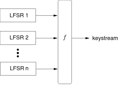
One general technique for destroying the linearity inherent in LFSRs is to use several LF-SRs in parallel. The keystream is generated as a nonlinear functionf of the outputs of the component LFSRs; this construction is illustrated in Figure 6.8. Such keystream generators are callednonlinear combination generators, andf is called thecombining function. The remainder of this subsection demonstrates that the functionf must satisfy several criteria in order to withstand certain particular cryptographic attacks.
LFSR 1
LFSR 2
LFSR n
f keystream
Figure 6.8:A nonlinear combination generator.fis a nonlinear combining function.
6.48 Definition A product ofmdistinct variables is called anmthorder productof the
vari-ables. Every Boolean functionf(x1, x2, . . . , xn)can be written as a modulo2sum of
dis-tinctmthorder products of its variables,0≤m≤n; this expression is called thealgebraic
normal formoff. Thenonlinear orderoff is the maximum of the order of the terms ap-pearing in its algebraic normal form.
For example, the Boolean functionf(x1, x2, x3, x4, x5) = 1⊕x2⊕x3⊕x4x5⊕
x1x3x4x5 has nonlinear order4. Note that the maximum possible nonlinear order of a
Boolean function innvariables isn. Fact 6.49 demonstrates that the output sequence of a nonlinear combination generator has high linear complexity, provided that a combining functionf of high nonlinear order is employed.
6.49 Fact Suppose thatnmaximum-length LFSRs, whose lengthsL1, L2, . . . , Lnare pairwise
distinct and greater than2, are combined by a nonlinear functionf(x1, x2, . . . , xn)(as in
Figure 6.8) which is expressed in algebraic normal form. Then the linear complexity of the keystream isf(L1, L2, . . . , Ln). (The expressionf(L1, L2, . . . , Ln)is evaluated over the
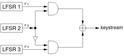
6.50 Example (Geffe generator) The Geffe generator, as depicted in Figure 6.9, is defined by three maximum-length LFSRs whose lengthsL1,L2,L3are pairwise relatively prime, with
nonlinear combining function
f(x1, x2, x3) = x1x2⊕(1 +x2)x3 = x1x2⊕x2x3⊕x3.
The keystream generated has period(2L1−1)·(2L2−1)·(2L3−1)and linear complexity
L=L1L2+L2L3+L3.
keystream
x1
x2
x3 LFSR 3 LFSR 2 LFSR 1
Figure 6.9:The Geffe generator.
The Geffe generator is cryptographically weak because information about the states of LFSR 1 and LFSR 3 leaks into the output sequence. To see this, letx1(t), x2(t), x3(t), z(t)
denote thetthoutput bits of LFSRs 1, 2, 3 and the keystream, respectively. Then the cor-relation probabilityof the sequencex1(t)to the output sequencez(t)is
P(z(t) =x1(t)) = P(x2(t) = 1) +P(x2(t) = 0)·P(x3(t) =x1(t))
= 1 2+
1 2·
1 2 =
3 4.
Similarly,P(z(t) = x3(t)) = 34. For this reason, despite having high period and
mod-erately high linear complexity, the Geffe generator succumbs to correlation attacks, as
de-scribed in Note 6.51.
6.51 Note (correlation attacks) Suppose thatnmaximum-length LFSRsR1, R2, . . . , Rn of
lengthsL1, L2, . . . , Lnare employed in a nonlinear combination generator. If the
connec-tion polynomials of the LFSRs and the combining funcconnec-tionf are public knowledge, then the number of different keys of the generator isn
i=1(2Li−1). (A key consists of the
ini-tial states of the LFSRs.) Suppose that there is a correlation between the keystream and the output sequence ofR1, with correlation probabilityp > 12. If a sufficiently long
seg-ment of the keystream is known (e.g., as is possible under a known-plaintext attack on a binary additive stream cipher), the initial state ofR1can be deduced by counting the
num-ber of coincidences between the keystream and all possible shifts of the output sequence ofR1, until this number agrees with the correlation probabilityp. Under these conditions,
finding the initial state ofR1will take at most2L1 −1trials. In the case where there is
a correlation between the keystream and the output sequences of each ofR1, R2, . . . , Rn,
the (secret) initial state of each LFSR can be determined independently in a total of about n
i=1(2Li −1)trials; this number is far smaller than the total number of different keys.
In a similar manner, correlations between the output sequences of particular subsets of the LFSRs and the keystream can be exploited.
the keystream. This condition can be satisfied iff is chosen to bemth-order correlation
immune.
6.52 Definition LetX1, X2, . . . , Xnbe independent binary variables, each taking on the
val-ues0or1with probability 12. A Boolean functionf(x1, x2, . . . , xn)ismth-order corre-lation immuneif for each subset ofmrandom variablesXi1, Xi2, . . . , Xim with1≤i1<
i2<· · ·< im≤n, the random variableZ =f(X1, X2, . . . , Xn)is statistically
indepen-dent of the random vector(Xi1, Xi2, . . . , Xim); equivalently,I(Z;Xi1, Xi2, . . . , Xim) =
0(see Definition 2.45).
For example, the functionf(x1, x2, . . . , xn) = x1⊕x2⊕ · · · ⊕xn is(n−1)th
-order correlation immune. In light of Fact 6.49, the following shows that there is a tradeoff between achieving high linear complexity and high correlation immunity with a combining function.
6.53 Fact If a Boolean functionf(x1, x2, . . . , xn)ismth-order correlation immune, where1≤
m < n, then the nonlinear order off is at mostn−m. Moreover, iff isbalanced(i.e., exactly half of the output values offare0) then the nonlinear order offis at mostn−m−1
for1≤m≤n−2.
The tradeoff between high linear complexity and high correlation immunity can be avoided by permittingmemoryin the nonlinear combination functionf. This point is il-lustrated by the summation generator.
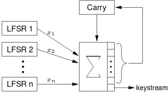
6.54 Example (summation generator) The combining function in the summation generator is based on the fact that integer addition, when viewed overZ2, is a nonlinear function with
memory whose correlation immunity is maximum. To see this in the casen= 2, leta=
am−12m−1+· · ·+a12+a0andb=bm−12m−1+· · ·+b12+b0be the binary representations
of integersaandb. Then the bits ofz=a+bare given by the recursive formula: zj = f1(aj, bj, cj−1) =aj⊕bj⊕cj−1 0≤j≤m,
cj = f2(aj, bj, cj−1) =ajbj⊕(aj⊕bj)cj−1, 0≤j≤m−1,
wherecjis the carry bit, andc−1 = am = bm = 0. Note thatf1is2nd-order
corre-lation immune, whilef2 is amemorylessnonlinear function. The carry bitcj−1 carries
all the nonlinear influence of less significant bits ofaandb(namely,aj−1, . . . , a1, a0and
bj−1, . . . , b1, b0).
The summation generator, as depicted in Figure 6.10, is defined bynmaximum-length LFSRs whose lengthsL1, L2, . . . , Lnare pairwise relatively prime. The secret key
con-keystream x1
x2
xn
LFSR 1
LFSR 2
LFSR n
Carry
sists of the initial states of the LFSRs, and an initial (integer) carryC0. The keystream
is generated as follows. At timej(j ≥ 1), the LFSRs are stepped producing output bits x1, x2, . . . , xn, and theintegersumSj =ni=1xi+Cj−1is computed. The keystream
bit isSjmod 2(the least significant bit ofSj), while the new carry is computed asCj =
⌊Sj/2⌋(the remaining bits ofSj). The period of the keystream isni=1(2Li−1), while its
linear complexity is close to this number.
Even though the summation generator has high period, linear complexity, and corre-lation immunity, it is vulnerable to certain correcorre-lation attacks and a known-plaintext attack
based on its2-adic span (see page 218).
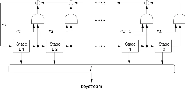
6.3.2 Nonlinear filter generators
Another general technique for destroying the linearity inherent in LFSRs is to generate the keystream as some nonlinear function of the stages of a single LFSR; this construction is illustrated in Figure 6.11. Such keystream generators are callednonlinear filter generators, andfis called thefiltering function.
Stage Stage
L-2
sj
L-1 1
c2
c1 cL−1 cL
f
keystream
Stage 0 Stage
Figure 6.11:A nonlinear filter generator.fis a nonlinear Boolean filtering function.
Fact 6.55 describes the linear complexity of the output sequence of a nonlinear filter generator.
6.55 Fact Suppose that a nonlinear filter generator is constructed using a maximum-length LFSR of lengthLand a filtering functionf of nonlinear orderm(as in Figure 6.11).
(i) (Key’s bound) The linear complexity of the keystream is at mostLm=mi=1
L i
. (ii) For a fixed maximum-length LFSR of prime lengthL, the fraction of Boolean
func-tionsf of nonlinear ordermwhich produce sequences of maximum linear complex-ityLmis
Pm ≈ exp(−Lm/(L·2L)) > e−1/L.
Therefore, for largeL, most of the generators produce sequences whose linear com-plexity meets the upper bound in (i).
6.56 Example (knapsack generator) The knapsack keystream generator is defined by a maxim-um-length LFSRL, C(D)and a modulusQ= 2L. The secret key consists ofLknapsack
integer weightsa1, a2, . . . , aLeach of bitlengthL, and the initial state of the LFSR.
Re-call that the subset sum problem (§3.10) is to determine a subset of the knapsack weights which add up to a given integers, provided that such a subset exists; this problem isNP -hard (Fact 3.91). The keystream is generated as follows: at timej, the LFSR is stepped and the knapsack sumSj =Li=1xiaimodQis computed, where[xL, . . . , x2, x1]is the
state of the LFSR at timej. Finally, selected bits ofSj(afterSjis converted to its binary
representation) are extracted to form part of the keystream (the⌈lgL⌉least significant bits ofSjshould be discarded). The linear complexity of the keystream is then virtually certain
to beL(2L−1).
Since the state of an LFSR is a binary vector, the function which maps the LFSR state to the knapsack sumSj is indeed nonlinear. Explicitly, let the functionf be defined by
f(x) = L
i=1xiaimodQ, wherex = [xL, . . . , x2, x1]is a state. Ifxandy are two
states then, in general,f(x⊕y)=f(x) +f(y).
6.3.3 Clock-controlled generators
In nonlinear combination generators and nonlinear filter generators, the component LFSRs are clocked regularly; i.e., the movement of data in all the LFSRs is controlled by the same clock. The main idea behind aclock-controlled generatoris to introduce nonlinearity into LFSR-based keystream generators by having the output of one LFSR control theclocking
(i.e., stepping) of a second LFSR. Since the second LFSR is clocked in an irregular manner, the hope is that attacks based on the regular motion of LFSRs can be foiled. Two clock-controlled generators are described in this subsection: (i) the alternating step generator and (ii) the shrinking generator.
(i) The alternating step generator
The alternating step generator uses an LFSRR1to control the stepping of two LFSRs,R2
andR3. The keystream produced is the XOR of the output sequences ofR2andR3.
6.57 AlgorithmAlternating step generator
SUMMARY: a control LFSRR1is used to selectively step two other LFSRs,R2andR3.
OUTPUT: a sequence which is the bitwise XOR of the output sequences ofR2andR3.
The following steps are repeated until a keystream of desired length is produced. 1. RegisterR1is clocked.
2. If the output ofR1is1then:
R2is clocked;R3is not clocked but its previous output bit is repeated.
(For the first clock cycle, the “previous output bit” ofR3is taken to be0.)
3. If the output ofR1is0then:
R3is clocked;R2is not clocked but its previous output bit is repeated.
(For the first clock cycle, the “previous output bit” ofR2is taken to be0.)
4. The output bits ofR2andR3are XORed; the resulting bit is part of the keystream.
More formally, let the output sequences of LFSRsR1,R2, andR3bea0, a1, a2, . . .,
b0, b1, b2, . . ., andc0, c1, c2. . ., respectively. Defineb−1=c−1= 0. Then the keystream
andt(j) = (j
i=0ai)−1for allj ≥ 0. The alternating step generator is depicted in
Figure 6.12.
LFSRR2
LFSRR3
LFSRR1 output
clock
Figure 6.12:The alternating step generator.
6.58 Example (alternating step generator with artificially small parameters) Consider an al-ternating step generator with component LFSRsR1 =3,1 +D2+D3,R2 = 4,1 +
D3+D4, andR
3=5,1 +D+D3+D4+D5. Suppose that the initial states ofR1,
R2, andR3are[0,0,1],[1,0,1,1], and[0,1,0,0,1], respectively. The output sequence of
R1is the7-periodic sequence with cycle
a7 = 1,0,0,1,0,1,1.
The output sequence ofR2is the15-periodic sequence with cycle
b15 = 1,1,0,1,0,1,1,1,1,0,0,0,1,0,0.
The output sequence ofR3is the31-periodic sequence with cycle
c31 = 1,0,0,1,0,1,0,1,1,0,0,0,0,1,1,1,0,0,1,1,0,1,1,1,1,1,0,1,0,0,0.
The keystream generated is
x = 1,0,1,1,1,0,1,0,1,0,1,0,0,0,0,1,0,1,1,1,1,0,1,1,0,0,0,1,1,1,0, . . . .
Fact 6.59 establishes, under the assumption thatR1produces a de Bruijn sequence (see
Definition 6.40), that the output sequence of an alternating step generator satisfies the basic requirements of high period, high linear complexity, and good statistical properties.
6.59 Fact (properties of the alternating step generator) Suppose thatR1produces a de Bruijn
sequence of period2L1. Furthermore, suppose thatR
2andR3are maximum-length LFSRs
of lengthsL2andL3, respectively, such thatgcd(L2, L3) = 1. Letxbe the output sequence
of the alternating step generator formed byR1,R2, andR3.
(i) The sequencexhas period2L1·(2L2−1)·(2L3−1).
(ii) The linear complexityL(x)ofxsatisfies
(L2+L3)·2L1−1 < L(x) ≤ (L2+L3)·2L1.
(iii) The distribution of patterns inxis almost uniform. More precisely, letP be any bi-nary string of lengthtbits, wheret≤min(L2, L3). Ifx(t)denotes anytconsecutive
bits inx, then the probability thatx(t) =Pis1
2
t
+O(1/2L2−t) +O(1/2L3−t).
high linear complexity, and good statistical properties in Fact 6.59 also hold whenR1is a
maximum-length LFSR. Note, however, that this has not yet been proven.
6.60 Note (security of the alternating step generator) The LFSRsR1,R2,R3should be
cho-sen to be maximum-length LFSRs whose lengthsL1,L2,L3are pairwise relatively prime:
gcd(L1, L2) = 1,gcd(L2, L3) = 1,gcd(L1, L3) = 1. Moreover, the lengths should be
about the same. IfL1 ≈l,L2 ≈l, andL3 ≈l, the best known attack on the alternating
step generator is a divide-and-conquer attack on the control registerR1 which takes
ap-proximately2lsteps. Thus, ifl≈128, the generator is secure against all presently known
attacks.
(ii) The shrinking generator
The shrinking generator is a relatively new keystream generator, having been proposed in 1993. Nevertheless, due to its simplicity and provable properties, it is a promising candi-date for high-speed encryption applications. In the shrinking generator, a control LFSRR1
is used to select a portion of the output sequence of a second LFSRR2. The keystream
produced is, therefore, ashrunkenversion (also known as anirregularly decimated subse-quence) of the output sequence ofR2, as specified in Algorithm 6.61 and depicted in
Fig-ure 6.13.
6.61 AlgorithmShrinking generator
SUMMARY: a control LFSRR1is used to control the output of a second LFSRR2.
The following steps are repeated until a keystream of desired length is produced. 1. RegistersR1andR2are clocked.
2. If the output ofR1is1, the output bit ofR2forms part of the keystream.
3. If the output ofR1is0, the output bit ofR2is discarded.
More formally, let the output sequences of LFSRs R1 andR2 bea0, a1, a2, . . . and
b0, b1, b2, . . ., respectively. Then the keystream produced by the shrinking generator is
x0, x1, x2, . . ., wherexj = bij, and, for eachj ≥0,ij is the position of thej
th1in the
sequencea0, a1, a2, . . ..
ai= 0
outputbi
discardbi
ai= 1
ai LFSRR1
LFSRR2
clock
bi
Figure 6.13:The shrinking generator.
6.62 Example (shrinking generator with artificially small parameters) Consider a shrinking generator with component LFSRsR1 =3,1 +D+D3andR2 =5,1 +D3+D5.
Suppose that the initial states ofR1andR2are[1,0,0]and[0,0,1,0,1], respectively. The
output sequence ofR1is the7-periodic sequence with cycle
while the output sequence ofR2is the31-periodic sequence with cycle
b31 = 1,0,1,0,0,0,0,1,0,0,1,0,1,1,0,0,1,1,1,1,1,0,0,0,1,1,0,1,1,1,0.
The keystream generated is
x = 1,0,0,0,0,1,0,1,1,1,1,1,0,1,1,1,0, . . . .
Fact 6.63 establishes that the output sequence of a shrinking generator satisfies the basic requirements of high period, high linear complexity, and good statistical properties.
6.63 Fact (properties of the shrinking generator) LetR1andR2be maximum-length LFSRs of
lengthsL1andL2, respectively, and letxbe an output sequence of the shrinking generator
formed byR1andR2.
(i) Ifgcd(L1, L2) = 1, thenxhas period(2L2−1)·2L1−1.
(ii) The linear complexityL(x)ofxsatisfies
L2·2L1−2 < L(x) ≤ L2·2L1−1.
(iii) Suppose that the connection polynomials forR1andR2are chosen uniformly at
ran-dom from the set of all primitive polynomials of degreesL1andL2overZ2. Then
the distribution of patterns inxis almost uniform. More precisely, ifP is any binary string of lengthtbits andx(t)denotes anytconsecutive bits inx, then the probability thatx(t) =Pis(12)t+O(t/2L2).
6.64 Note (security of the shrinking generator) Suppose that the component LFSRsR1andR2
of the shrinking generator have lengthsL1andL2, respectively. If the connection
polyno-mials forR1andR2are known (but not the initial contents ofR1andR2), the best attack
known for recovering the secret key takesO(2L1·L3
2)steps. On the other hand, if secret
(and variable) connection polynomials are used, the best attack known takesO(22L1·L
1·
L2)steps. There is also an attack through the linear complexity of the shrinking generator
which takesO(2L1·L2
2)steps (regardless of whether the connections are known or secret),
but this attack requires2L1·L
2consecutive bits from the output sequence and is, therefore,
infeasible for moderately largeL1andL2. For maximum security,R1andR2should be
maximum-length LFSRs, and their lengths should satisfygcd(L1, L2) = 1. Moreover,
se-cret connections should be used. Subject to these constraints, ifL1 ≈landL2 ≈l, the
shrinking generator has a security level approximately equal to22l. Thus, ifL
1 ≈64and
L2≈64, the generator appears to be secure against all presently known attacks.
6.4 Other stream ciphers
While the LFSR-based stream ciphers discussed in§6.3 are well-suited to hardware im-plementation, they are not especially amenable to software implementation. This has led to several recent proposals for stream ciphers designed particularly for fast software imple-mentation. Most of these proposals are either proprietary, or are relatively new and have not received sufficient scrutiny from the cryptographic community; for this reason, they are not presented in this section, and instead only mentioned in the chapter notes on page 222.
other widely used stream ciphers not based on LFSRs are the Output Feedback (OFB; see §7.2.2(iv)) and Cipher Feedback (CFB; see§7.2.2(iii)) modes of block ciphers. Another class of keystream generators not based on LFSRs are those whose security relies on the intractability of an underlying number-theoretic problem; these generators are much slower than those based on LFSRs and are discussed in§5.5.
6.4.1 SEAL
SEAL (Software-optimized Encryption Algorithm) is a binary additive stream cipher (see Definition 6.4) that was proposed in 1993. Since it is relatively new, it has not yet received much scrutiny from the cryptographic community. However, it is presented here because it is one of the few stream ciphers that was specifically designed for efficient software im-plementation and, in particular, for 32-bit processors.
SEAL is a length-increasing pseudorandom function which maps a 32-bitsequence numbernto anL-bit keystream under control of a 160-bit secret keya. In the preprocess-ing stage (step 1 of Algorithm 6.68), the key is stretched into larger tables uspreprocess-ing the table-generation functionGaspecified in Algorithm 6.67; this function is based on the Secure
Hash Algorithm SHA-1 (Algorithm 9.53). Subsequent to this preprocessing, keystream generation requires about 5 machine instructions per byte, and is an order of magnitude faster than DES (Algorithm 7.82).
The following notation is used in SEAL for 32-bit quantitiesA,B,C,D,Xi, andYj:
• A: bitwise complement ofA
• A∧B,A∨B,A⊕B: bitwise AND, inclusive-OR, exclusive-OR • “A←֓ s”:32-bit result of rotatingAleft throughspositions • “A ֒→s”:32-bit result of rotatingAright throughspositions • A+B: mod232sum of the unsigned integersAandB
• f(B, C, D)def= (B∧C)∨(B∧D); g(B, C, D)def= (B∧C)∨(B∧D)∨(C∧D);
h(B, C, D)def= B⊕C⊕D • AB: concatenation ofAandB
• (X1, . . . , Xj)←(Y1, . . . , Yj): simultaneous assignments(Xi←Yi), where
(Y1, . . . , Yj)is evaluated prior to any assignments.
6.65 Note (SEAL 1.0 vs. SEAL 2.0) The table-generation function (Algorithm 6.67) for the first version of SEAL (SEAL 1.0) was based on the Secure Hash Algorithm (SHA). SEAL 2.0 differs from SEAL 1.0 in that the table-generation function for the former is based on the modified Secure Hash Algorithm SHA-1 (Algorithm 9.53).
6.67 AlgorithmTable-generation function for SEAL 2.0
Ga(i)
INPUT: a 160-bit stringaand an integeri,0≤i <232.
OUTPUT: a 160-bit string, denotedGa(i).
1. Definition of constants. Define four 32-bit constants (in hex): y1 =0x5a827999,
y2=0x6ed9eba1,y3=0x8f1bbcdc,y4=0xca62c1d6.
2. Table-generation function.
(initialize8032-bit wordsX0, X1, . . . , X79)
SetX0←i. Forjfrom1to15do:Xj←0x00000000.
Forjfrom16to79do:Xj ←((Xj−3⊕Xj−8⊕Xj−14⊕Xj−16)←֓1).
(initialize working variables)
Break up the 160-bit stringainto five 32-bit words:a=H0H1H2H3H4.
(A, B, C, D, E)←(H0, H1, H2, H3, H4).
(execute four rounds of 20 steps, then update;tis a temporary variable) (Round 1) Forjfrom0to19do the following:
t ←((A←֓5) +f(B, C, D) +E+Xj+y1),
(A, B, C, D, E)←(t, A, B←֓30, C, D). (Round 2) Forjfrom20to39do the following: t ←((A←֓5) +h(B, C, D) +E+Xj+y2),
(A, B, C, D, E)←(t, A, B←֓30, C, D). (Round 3) Forjfrom40to59do the following: t ←((A←֓5) +g(B, C, D) +E+Xj+y3),
(A, B, C, D, E)←(t, A, B←֓30, C, D). (Round 4) Forjfrom60to79do the following: t ←((A←֓5) +h(B, C, D) +E+Xj+y4),
(A, B, C, D, E)←(t, A, B←֓30, C, D). (update chaining values)
(H0, H1, H2, H3, H4)←(H0+A, H1+B, H2+C, H3+D, H4+E).
(completion) The value ofGa(i)is the 160-bit stringH0H1H2H3H4.
6.68 AlgorithmKeystream generator for SEAL 2.0
SEAL(a,n)
INPUT: a 160-bit stringa(the secret key), a (non-secret) integern,0 ≤ n < 232(the
sequence number), and the desired bitlengthLof the keystream.
OUTPUT: keystreamyof bitlengthL′, whereL′is the least multiple of 128 which is≥L. 1. Table generation. Generate the tablesT,S, andR, whose entries are 32-bit words. The functionFused below is defined byFa(i) =Hiimod5, whereH0iH1iH2iH3iH4i =
Ga(⌊i/5⌋), and where the functionGais defined in Algorithm 6.67.
1.1 Forifrom0to511do the following:T[i]←Fa(i).
1.2 Forjfrom0to255do the following:S[j]←Fa(0x00001000+j).
1.3 Forkfrom0to4· ⌈(L−1)/8192⌉ −1do:R[k]←Fa(0x00002000+k).
2. Initialization procedure.The following is a description of the subroutine
Initialize(n, l, A, B, C, D, n1, n2, n3, n4) which takes as input a 32-bit wordn
and an integerl, and outputs eight 32-bit wordsA,B,C,D,n1,n2,n3, andn4. This
subroutine is used in step 4.
Forjfrom1to2do the following:
P←A∧0x000007fc, B←B+T[P/4], A←(A ֒→9), P←B∧0x000007fc, C←C+T[P/4], B←(B ֒→9), P←C∧0x000007fc, D←D+T[P/4], C←(C ֒→9), P←D∧0x000007fc, A←A+T[P/4], D←(D ֒→9).
(n1, n2, n3, n4)←(D, B, A, C).
P←A∧0x000007fc, B←B+T[P/4], A←(A ֒→9). P←B∧0x000007fc, C←C+T[P/4], B←(B ֒→9). P←C∧0x000007fc, D←D+T[P/4], C←(C ֒→9). P←D∧0x000007fc, A←A+T[P/4], D←(D ֒→9). 3. Initializeyto be the empty string, andl←0.
4. Repeat the following:
4.1 Execute the procedureInitialize(n, l, A, B, C, D, n1, n2, n3, n4).
4.2 Forifrom1to64do the following:
P←A∧0x000007fc, B←B+T[P/4], A←(A ֒→9), B←B⊕A, Q←B∧0x000007fc, C←C⊕T[Q/4], B←(B ֒→9), C←C+B, P←(P+C)∧0x000007fc, D←D+T[P/4], C←(C ֒→9), D←D⊕C, Q←(Q+D)∧0x000007fc, A←A⊕T[Q/4], D←(D ֒→9), A←A+D, P←(P+A)∧0x000007fc, B←B⊕T[P/4], A←(A ֒→9),
Q←(Q+B)∧0x000007fc, C←C+T[Q/4], B←(B ֒→9), P←(P+C)∧0x000007fc, D←D⊕T[P/4], C←(C ֒→9), Q←(Q+D)∧0x000007fc, A←A+T[Q/4], D←(D ֒→9),
y←y(B+S[4i−4])(C⊕S[4i−3])(D+S[4i−2])(A⊕S[4i−1]). Ifyis≥Lbits in length then return(y) and stop.
Ifiis odd, set(A, C)←(A+n1, C+n2). Otherwise,(A, C)←(A+n3, C+n4).
4.3 Setl←l+ 1.
6.69 Note (choice of parameterL) In most applications of SEAL 2.0 it is expected thatL ≤
219; larger values ofLare permissible, but come at the expense of a larger tableR. A
preferred method for generating a longer keystream without requiring a larger tableRis to compute the concatenation of the keystreams SEAL(a,0), SEAL(a,1), SEAL(a,2),. . .. Since the sequence number isn <232, a keystream of length up to251bits can be obtained
in this manner withL= 219.
6.70 Example (test vectors for SEAL 2.0) Suppose the keyais the 160-bit (hexadecimal) string
67452301 efcdab89 98badcfe 10325476 c3d2e1f0,
n=0x013577af, andL= 32768bits. TableRconsists of wordsR[0], R[1], . . . , R[15]:
5021758d ce577c11 fa5bd5dd 366d1b93 182cff72 ac06d7c6 2683ead8 fabe3573 82a10c96 48c483bd ca92285c 71fe84c0 bd76b700 6fdcc20c 8dada151 4506dd64
The tableT consists of wordsT[0], T[1], . . . , R[511]:
The tableSconsists of wordsS[0], S[1], . . . , S[255]:
907c1e3d ce71ef0a 48f559ef 2b7ab8bc 4557f4b8 033e9b05 4fde0efa 1a845f94 38512c3b d4b44591 53765dce 469efa02 ... ... ... ... ... ... bd7dea87 fd036d87 53aa3013 ec60e282 1eaef8f9 0b5a0949
The outputyof Algorithm 6.68 consists of 1024 wordsy[0], y[1], . . . , y[1023]:
37a00595 9b84c49c a4be1e05 0673530f 0ac8389d c5878ec8 da6666d0 6da71328 1419bdf2 d258bebb b6a42a4d 8a311a72 ... ... ... ... ... ... 547dfde9 668d50b5 ba9e2567 413403c5 43120b5a ecf9d062
The XOR of the 1024 words ofyis 0x098045fc.
6.5 Notes and further references
§6.1
Although now dated, Rueppel [1075] provides a solid introduction to the analysis and design of stream ciphers. For an updated and more comprehensive survey, see Rueppel [1081]. Another recommended survey is that of Robshaw [1063].
The concept of unconditional security was introduced in the seminal paper by Shannon [1120]. Maurer [819] surveys the role of information theory in cryptography and, in partic-ular, secrecy, authentication, and secret sharing schemes. Maurer [811] devised a random-ized stream cipherthat is unconditionally secure “with high probability”. More precisely, an adversary is unable to obtain any information whatsoever about the plaintext with prob-ability arbitrarily close to1, unless the adversary can perform an infeasible computation. The cipher utilizes a publicly-accessible source of random bits whose length is much greater than that of all the plaintext to be encrypted, and can conceivably be made practical. Mau-rer’s cipher is based on the impracticalRip van Winkle cipherof Massey and Ingermarsson [789], which is described by Rueppel [1081].
One technique for solving the re-synchronization problem with synchronous stream ciphers is to have the receiver send a resynchronization request to the sender, whereby a new inter-nal state is computed as a (public) function of the origiinter-nal interinter-nal state (or key) and some public information (such as the time at the moment of the request). Daemen, Govaerts, and Vandewalle [291] showed that this approach can result in a total loss of security for some published stream cipher proposals. Proctor [1011] considered the trade-off between the security and error propagation problems that arise by varying the number of feedback ciphertext digits. Maurer [808] presented various design approaches for self-synchronizing stream ciphers that are potentially superior to designs based on block ciphers, both with re-spect to encryption speed and security.
§6.2
An excellent introduction to the theory of both linear and nonlinear shift registers is the book by Golomb [498]; see also Selmer [1107], Chapters 5 and 6 of Beker and Piper [84], and Chapter 8 of Lidl and Niederreiter [764]. A lucid treatment ofm-sequences can be found in Chapter 10 of McEliece [830]. While the discussion in this chapter has been restricted to se-quences and feedback shift registers over the binary fieldZ2, many of the results presented
The results on the expected linear complexity and linear complexity profile of random se-quences (Facts 6.21, 6.22, 6.24, and 6.25) are from Chapter 4 of Rueppel [1075]; they also appear in Rueppel [1077]. Dai and Yang [294] extended Fact 6.22 and obtained bounds for the expected linear complexity of ann-periodic sequence for each possible value ofn. The bounds imply that the expected linear complexity of a random periodic sequence is close to the period of the sequence. The linear complexity profile of the sequence defined in Example 6.27 was established by Dai [293]. For further theoretical analysis of the linear complexity profile, consult the work of Niederreiter [927, 928, 929, 930].
Facts 6.29 and 6.34 are due to Massey [784]. The Berlekamp-Massey algorithm (Algo-rithm 6.30) is due to Massey [784], and is based on an earlier algo(Algo-rithm of Berlekamp [118] for decoding BCH codes. While the algorithm in§6.2.3 is only described for binary se-quences, it can be generalized to find the linear complexity of sequences over any field. Further discussion and refinements of the Berlekamp-Massey algorithm are given by Blahut [144]. There are numerous other algorithms for computing the linear complexity of a se-quence. For example, Games and Chan [439] and Robshaw [1062] present efficient algo-rithms for determining the linear complexity of binary sequences of period2n; these
algo-rithms have limited practical use since they require an entire cycle of the sequence.
Jansen and Boekee [632] defined themaximum order complexityof a sequence to be the length of the shortest (not necessarily linear) feedback shift register (FSR) that can gener-ate the sequence. The expected maximum order complexity of a random binary sequence of lengthnis approximately2 lgn. An efficient linear-time algorithm for computing this complexity measure was also presented; see also Jansen and Boekee [631].
Another complexity measure, theZiv-Lempel complexity measure, was proposed by Ziv and Lempel [1273]. This measure quantifies the rate at which new patterns appear in a sequence. Mund [912] used a heuristic argument to derive the expected Ziv-Lempel complexity of a random binary sequence of a given length. For a detailed study of the relative strengths and weaknesses of the linear, maximum order, and Ziv-Lempel complexity measures, see Erdmann [372].
Kolmogorov [704] and Chaitin [236] introduced the notion of so-calledTuring-Kolmogorov -Chaitin complexity, which measures the minimum size of the input to a fixed universal Turing machine which can generate a given sequence; see also Martin-L¨of [783]. While this complexity measure is of theoretical interest, there is no algorithm known for computing it and, hence, it has no apparent practical significance. Beth and Dai [124] have shown that the Turing-Kolmogorov-Chaitin complexity is approximately twice the linear complexity for most sequences of sufficient length.
Fact 6.39 is due to Golomb and Welch, and appears in the book of Golomb [498, p.115]. Lai [725] showed that Fact 6.39 is only true for the binary case, and established necessary and sufficient conditions for an FSR over a general finite field to be nonsingular.