For further information, see
www.cacr.math.uwaterloo.ca/hac
CRC Press has granted the following specific permissions for the electronic version of this
book:
Permission is granted to retrieve, print and store a single copy of this chapter for
personal use. This permission does not extend to binding multiple chapters of
the book, photocopying or producing copies for other than personal use of the
person creating the copy, or making electronic copies available for retrieval by
others without prior permission in writing from CRC Press.
Except where over-ridden by the specific permission above, the standard copyright notice
from CRC Press applies to this electronic version:
Neither this book nor any part may be reproduced or transmitted in any form or
by any means, electronic or mechanical, including photocopying, microfilming,
and recording, or by any information storage or retrieval system, without prior
permission in writing from the publisher.
The consent of CRC Press does not extend to copying for general distribution,
for promotion, for creating new works, or for resale. Specific permission must be
obtained in writing from CRC Press for such copying.
c
§1.11
One approach to distributing public-keys is the so-called Merkle channel (see Simmons [1144, p.387]). Merkle proposed that public keys be distributed over so many independent public channels (newspaper, radio, television, etc.) that it would be improbable for an ad-versary to compromise all of them.
In 1979 Kohnfelder [702] suggested the idea of using public-key certificates to facilitate the distribution of public keys over unsecured channels, such that their authenticity can be verified. Essentially the same idea, but by on-line requests, was proposed by Needham and Schroeder (ses Wilkes [1244]).
A provably secure key agreement protocol has been proposed whose security is based on the Heisenberg uncertainty principle of quantum physics. The security of so-called quantum
cryptography does not rely upon any complexity-theoretic assumptions. For further details
on quantum cryptography, consult Chapter 6 of Brassard [192], and Bennett, Brassard, and Ekert [115].
§1.12
For an introduction and detailed treatment of many pseudorandom sequence generators, see Knuth [692]. Knuth cites an example of a complex scheme to generate random numbers which on closer analysis is shown to produce numbers which are far from random, and con-cludes: ...random numbers should not be generated with a method chosen at random.
§1.13
Mathematical Background
Contents in Brief
2.1 Probability theory. . . 50
2.2 Information theory . . . 56
2.3 Complexity theory . . . 57
2.4 Number theory . . . 63
2.5 Abstract algebra . . . 75
2.6 Finite fields . . . 80
2.7 Notes and further references . . . 85
This chapter is a collection of basic material on probability theory, information the-ory, complexity thethe-ory, number thethe-ory, abstract algebra, and finite fields that will be used throughout this book. Further background and proofs of the facts presented here can be found in the references given in§2.7. The following standard notation will be used through-out:
1. Zdenotes the set of integers; that is, the set{. . . ,−2,−1,0,1,2, . . .}. 2. Qdenotes the set of rational numbers; that is, the set{ab |a, b∈Z, b6= 0}. 3. Rdenotes the set of real numbers.
4. πis the mathematical constant;π≈3.14159. 5. eis the base of the natural logarithm;e≈2.71828. 6. [a, b]denotes the integersxsatisfyinga≤x≤b.
7. ⌊x⌋is the largest integer less than or equal tox. For example,⌊5.2⌋= 5and
⌊−5.2⌋=−6.
8. ⌈x⌉is the smallest integer greater than or equal tox. For example,⌈5.2⌉= 6and
⌈−5.2⌉=−5.
9. IfAis a finite set, then|A|denotes the number of elements inA, called the cardinality ofA.
10. a∈Ameans that elementais a member of the setA. 11. A⊆Bmeans thatAis a subset ofB.
12. A⊂Bmeans thatAis a proper subset ofB; that isA⊆BandA6=B. 13. The intersection of setsAandBis the setA∩B={x|x∈Aandx∈B}. 14. The union of setsAandBis the setA∪B={x|x∈Aorx∈B}. 15. The difference of setsAandBis the setA−B={x|x∈Aandx6∈B}. 16. The Cartesian product of setsAandBis the setA×B={(a, b)|a∈Aandb∈
17. A function or mappingf :A−→Bis a rule which assigns to each elementainA
precisely one elementbinB. Ifa∈Ais mapped tob∈Bthenbis called the image ofa,ais called a preimage ofb, and this is writtenf(a) =b. The setAis called the
domain off, and the setBis called the codomain off.
18. A functionf :A−→Bis1−1(one-to-one) or injective if each element inBis the image of at most one element inA. Hencef(a1) =f(a2)impliesa1=a2.
19. A functionf :A −→Bis onto or surjective if eachb ∈Bis the image of at least onea∈A.
20. A functionf : A −→ B is a bijection if it is both one-to-one and onto. Iff is a bijection between finite setsAandB, then|A|=|B|. Iff is a bijection between a setAand itself, thenf is called a permutation onA.
21. lnxis the natural logarithm ofx; that is, the logarithm ofxto the basee. 22. lgxis the logarithm ofxto the base2.
23. exp(x)is the exponential functionex.
24. Pni=1aidenotes the suma1+a2+· · ·+an.
25. Qni=1aidenotes the producta1·a2· · · · ·an.
26. For a positive integern, the factorial function isn! = n(n−1)(n−2)· · ·1. By convention,0! = 1.
2.1 Probability theory
2.1.1 Basic definitions
2.1 Definition An experiment is a procedure that yields one of a given set of outcomes. The individual possible outcomes are called simple events. The set of all possible outcomes is called the sample space.
This chapter only considers discrete sample spaces; that is, sample spaces with only finitely many possible outcomes. Let the simple events of a sample spaceS be labeled
s1, s2, . . . , sn.
2.2 Definition A probability distributionPonSis a sequence of numbersp1, p2, . . . , pnthat
are all non-negative and sum to 1. The numberpiis interpreted as the probability ofsibeing
the outcome of the experiment.
2.3 Definition An eventEis a subset of the sample spaceS. The probability that eventE
occurs, denotedP(E), is the sum of the probabilitiespiof all simple eventssiwhich belong
toE. Ifsi∈S,P({si})is simply denoted byP(si).
2.4 Definition IfEis an event, the complementary event is the set of simple events not be-longing toE, denotedE.
2.5 Fact LetE⊆Sbe an event.
(iii) If the outcomes inSare equally likely, thenP(E) =||ES||.
2.6 Definition Two eventsE1andE2are called mutually exclusive ifP(E1∩E2) = 0. That
is, the occurrence of one of the two events excludes the possibility that the other occurs.
2.7 Fact LetE1andE2be two events.
(i) IfE1⊆E2, thenP(E1)≤P(E2).
(ii) P(E1∪E2) +P(E1∩E2) =P(E1) +P(E2). Hence, ifE1andE2are mutually
exclusive, thenP(E1∪E2) =P(E1) +P(E2).
2.1.2 Conditional probability
2.8 Definition LetE1andE2be two events withP(E2)>0. The conditional probability of E1givenE2, denotedP(E1|E2), is
P(E1|E2) =
P(E1∩E2) P(E2) .
P(E1|E2)measures the probability of eventE1occurring, given thatE2has occurred. 2.9 Definition EventsE1andE2are said to be independent ifP(E1∩E2) =P(E1)P(E2).
Observe that ifE1andE2are independent, thenP(E1|E2) =P(E1)andP(E2|E1) = P(E2). That is, the occurrence of one event does not influence the likelihood of occurrence
of the other.
2.10 Fact (Bayes’ theorem) IfE1andE2are events withP(E2)>0, then P(E1|E2) = P(E1)P(E2|E1)
P(E2) .
2.1.3 Random variables
LetSbe a sample space with probability distributionP.
2.11 Definition A random variableX is a function from the sample spaceSto the set of real numbers; to each simple eventsi∈S,Xassigns a real numberX(si).
SinceSis assumed to be finite,X can only take on a finite number of values.
2.12 DefinitionP LetXbe a random variable onS. The expected value or mean ofXisE(X) =
si∈SX(si)P(si).
2.13 Fact LetXbe a random variable onS. ThenE(X) =Px∈Rx·P(X =x).
2.14 Fact IfX1, X2, . . . , Xmare random variables onS, anda1, a2, . . . , amare real numbers,
thenE(Pmi=1aiXi) =Pmi=1aiE(Xi).
2.15 Definition The variance of a random variableXof meanµis a non-negative number de-fined by
Var(X) =E((X−µ)2).
If a random variable has small variance then large deviations from the mean are un-likely to be observed. This statement is made more precise below.
2.16 Fact (Chebyshev’s inequality) LetX be a random variable with meanµ = E(X)and varianceσ2= Var(X). Then for anyt >0,
P(|X−µ| ≥t)≤ σ 2
t2.
2.1.4 Binomial distribution
2.17 Definition Letnandkbe non-negative integers. The binomial coefficient nkis the num-ber of different ways of choosingkdistinct objects from a set ofndistinct objects, where the order of choice is not important.
2.18 Fact (properties of binomial coefficients) Letnandkbe non-negative integers. (i) nk= n!
k!(n−k)!.
(ii) nk= n−nk.
(iii) nk+1+1= nk+ k+1n .
2.19 Fact (binomial theorem) For any real numbersa,b, and non-negative integern,(a+b)n=
Pn k=0 nk
akbn−k.
2.20 Definition A Bernoulli trial is an experiment with exactly two possible outcomes, called
success and failure.
2.21 Fact Suppose that the probability of success on a particular Bernoulli trial isp. Then the probability of exactlyksuccesses in a sequence ofnsuch independent trials is
n
k
pk(1−p)n−k, for each0≤k≤n. (2.1)
2.22 Definition The probability distribution (2.1) is called the binomial distribution.
2.23 Fact The expected number of successes in a sequence ofnindependent Bernoulli trials, with probabilitypof success in each trial, isnp. The variance of the number of successes isnp(1−p).
2.24 Fact (law of large numbers) LetXbe the random variable denoting the fraction of suc-cesses innindependent Bernoulli trials, with probabilitypof success in each trial. Then for anyǫ >0,
P(|X−p|> ǫ)−→0, asn−→ ∞.
2.1.5 Birthday problems
2.25 Definition
(i) For positive integersm,nwithm≥n, the numberm(n)is defined as follows: m(n)=m(m−1)(m−2)· · ·(m−n+ 1).
(ii) Letm, nbe non-negative integers withm≥ n. The Stirling number of the second
kind, denotedmn , is
The symbolmn counts the number of ways of partitioning a set ofmobjects inton
non-empty subsets.
2.26 Fact (classical occupancy problem) An urn hasmballs numbered1tom. Suppose thatn
balls are drawn from the urn one at a time, with replacement, and their numbers are listed. The probability that exactlytdifferent balls have been drawn is
P1(m, n, t) =
n
t
m(t)
mn , 1≤t≤n.
The birthday problem is a special case of the classical occupancy problem.
2.27 Fact (birthday problem) An urn hasmballs numbered1tom. Suppose thatnballs are drawn from the urn one at a time, with replacement, and their numbers are listed.
(i) The probability of at least one coincidence (i.e., a ball drawn at least twice) is
P2(m, n) = 1−P1(m, n, n) = 1− The following explains why probability distribution (2.2) is referred to as the birthday
surprise or birthday paradox. The probability that at least2people in a room of23people have the same birthday isP2(365,23)≈0.507, which is surprisingly large. The quantity P2(365, n)also increases rapidly asnincreases; for example,P2(365,30)≈0.706.
A different kind of problem is considered in Facts 2.28, 2.29, and 2.30 below. Suppose that there are two urns, one containingmwhite balls numbered1tom, and the other con-tainingmred balls numbered1tom. First,n1balls are selected from the first urn and their
numbers listed. Thenn2balls are selected from the second urn and their numbers listed.
Finally, the number of coincidences between the two lists is counted.
2.28 Fact (model A) If the balls from both urns are drawn one at a time, with replacement, then the probability of at least one coincidence is
where the summation is over all0≤t1≤n1,0≤t2≤n2. Ifn=n1=n2,n=O(√m)
2.29 Fact (model B) If the balls from both urns are drawn without replacement, then the prob-ability of at least one coincidence is
P4(m, n1, n2) = 1−
2.30 Fact (model C) If then1white balls are drawn one at a time, with replacement, and then2
red balls are drawn without replacement, then the probability of at least one coincidence is
P5(m, n1, n2) = 1−
2.31 Definition LetFndenote the collection of all functions (mappings) from a finite domain
of sizento a finite codomain of sizen.
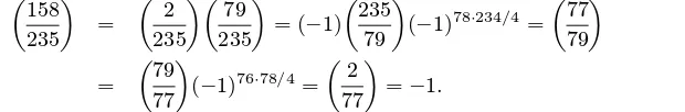
Models where random elements of Fn are considered are called random mappings
models. In this section the only random mappings model considered is where every function
fromFnis equally likely to be chosen; such models arise frequently in cryptography and
algorithmic number theory. Note that|Fn|=nn, whence the probability that a particular
function fromFnis chosen is1/nn.
2.32 Definition Letf be a function inFnwith domain and codomain equal to{1,2, . . . , n}.
The functional graph off is a directed graph whose points (or vertices) are the elements
{1,2, . . . , n}and whose edges are the ordered pairs(x, f(x))for allx∈ {1,2, . . . , n}.
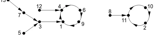
2.33 Example (functional graph) Consider the functionf :{1,2, . . . ,13} −→ {1,2, . . . ,13}
defined byf(1) = 4,f(2) = 11,f(3) = 1,f(4) = 6,f(5) = 3,f(6) = 9,f(7) = 3,
f(8) = 11,f(9) = 1,f(10) = 2,f(11) = 10,f(12) = 4,f(13) = 7. The functional
graph off is shown in Figure 2.1.
As Figure 2.1 illustrates, a functional graph may have several components (maximal connected subgraphs), each component consisting of a directed cycle and some directed
trees attached to the cycle.
2.34 Fact Asntends to infinity, the following statements regarding the functional digraph of a random functionffromFnare true:
13 7
5
3
12 4
1 9
6 8
11 2
10
Figure 2.1:A functional graph (see Example 2.33).
(ii) The expected number of points which are on the cycles ispπn/2.
(iii) The expected number of terminal points (points which have no preimages) isn/e. (iv) The expected number ofk-th iterate image points (xis ak-th iterate image point if
x=f(f(· · ·f
| {z }
ktimes
(y)· · ·))for somey) is(1−τk)n, where theτksatisfy the recurrence
τ0= 0,τk+1=e−1+τkfork≥0.
2.35 Definition Letf be a random function from{1,2, . . . , n}to{1,2, . . . , n}and letu ∈ {1,2, . . . , n}. Consider the sequence of pointsu0, u1, u2, . . . defined byu0 = u,ui =
f(ui−1)fori≥1. In terms of the functional graph off, this sequence describes a path that
connects to a cycle.
(i) The number of edges in the path is called the tail length ofu, denotedλ(u). (ii) The number of edges in the cycle is called the cycle length ofu, denotedµ(u). (iii) The rho-length ofuis the quantityρ(u) =λ(u) +µ(u).
(iv) The tree size ofuis the number of edges in the maximal tree rooted on a cycle in the component that containsu.
(v) The component size ofuis the number of edges in the component that containsu. (vi) The predecessors size ofuis the number of iterated preimages ofu.
2.36 Example The functional graph in Figure 2.1 has2components and4terminal points. The pointu = 3has parametersλ(u) = 1,µ(u) = 4,ρ(u) = 5. The tree, component, and predecessors sizes ofu= 3are4,9, and3, respectively.
2.37 Fact Asntends to infinity, the following are the expectations of some parameters associ-ated with a random point in{1,2, . . . , n}and a random function fromFn: (i) tail length:
p
πn/8(ii) cycle length: pπn/8(iii) rho-length:pπn/2(iv) tree size: n/3(v) compo-nent size:2n/3(vi) predecessors size:pπn/8.
2.38 Fact Asntends to infinity, the expectations of the maximum tail, cycle, and rho lengths in a random function fromFnarec1√n,c2√n, andc3√n, respectively, wherec1≈0.78248, c2≈1.73746, andc3≈2.4149.
2.2 Information theory
2.2.1 Entropy
LetXbe a random variable which takes on a finite set of valuesx1, x2, . . . , xn, with
prob-abilityP(X =xi) =pi, where0≤pi≤1for eachi,1≤i≤n, and wherePni=1pi = 1.
Also, letY andZbe random variables which take on finite sets of values.
The entropy ofXis a mathematical measure of the amount of information provided by an observation ofX. Equivalently, it is the uncertainity about the outcome before an obser-vation ofX. Entropy is also useful for approximating the average number of bits required to encode the elements ofX.
2.39 Definition The entropy or uncertainty ofX is defined to beH(X) =−Pni=1pilgpi=
Pn i=1pilg
1
pi
where, by convention,pi·lgpi=pi·lg
1
pi
= 0ifpi= 0.
2.40 Fact (properties of entropy) LetXbe a random variable which takes onnvalues. (i) 0≤H(X)≤lgn.
(ii) H(X) = 0if and only ifpi= 1for somei, andpj= 0for allj6=i(that is, there is
no uncertainty of the outcome).
(iii) H(X) = lgnif and only ifpi = 1/nfor eachi,1≤i≤n(that is, all outcomes are
equally likely).
2.41 Definition The joint entropy ofXandY is defined to be
H(X, Y) =−X
x,y
P(X=x, Y =y) lg(P(X =x, Y =y)),
where the summation indicesxandyrange over all values ofXandY, respectively. The definition can be extended to any number of random variables.
2.42 Fact IfXandY are random variables, thenH(X, Y)≤H(X) +H(Y), with equality if and only ifXandY are independent.
2.43 Definition IfX,Y are random variables, the conditional entropy ofX givenY =yis
H(X|Y =y) =−X
x
P(X =x|Y =y) lg(P(X =x|Y =y)),
where the summation indexxranges over all values ofX. The conditional entropy ofX givenY, also called the equivocation of Y aboutX, is
H(X|Y) =X
y
P(Y =y)H(X|Y =y),
where the summation indexyranges over all values ofY.
2.44 Fact (properties of conditional entropy) LetXandY be random variables.
(i) The quantityH(X|Y)measures the amount of uncertainty remaining aboutXafter
(ii) H(X|Y)≥0andH(X|X) = 0.
(iii) H(X, Y) =H(X) +H(Y|X) =H(Y) +H(X|Y).
(iv) H(X|Y)≤H(X), with equality if and only ifXandY are independent.
2.2.2 Mutual information
2.45 Definition The mutual information or transinformation of random variablesXandY is
I(X;Y) = H(X)−H(X|Y). Similarly, the transinformation ofXand the pairY,Z is defined to beI(X;Y, Z) =H(X)−H(X|Y, Z).
2.46 Fact (properties of mutual transinformation)
(i) The quantityI(X;Y)can be thought of as the amount of information thatY reveals aboutX. Similarly, the quantityI(X;Y, Z)can be thought of as the amount of in-formation thatY andZtogether reveal aboutX.
(ii) I(X;Y)≥0.
(iii) I(X;Y) = 0if and only ifX andY are independent (that is,Y contributes no in-formation aboutX).
(iv) I(X;Y) =I(Y;X).
2.47 Definition The conditional transinformation of the pairX,Y givenZis defined to be
IZ(X;Y) =H(X|Z)−H(X|Y, Z).
2.48 Fact (properties of conditional transinformation)
(i) The quantityIZ(X;Y)can be interpreted as the amount of information thatY
pro-vides aboutX, given thatZhas already been observed. (ii) I(X;Y, Z) =I(X;Y) +IY(X;Z).
(iii) IZ(X;Y) =IZ(Y;X).
2.3 Complexity theory
2.3.1 Basic definitions
The main goal of complexity theory is to provide mechanisms for classifying computational problems according to the resources needed to solve them. The classification should not depend on a particular computational model, but rather should measure the intrinsic dif-ficulty of the problem. The resources measured may include time, storage space, random bits, number of processors, etc., but typically the main focus is time, and sometimes space.
Of course, the term “well-defined computational procedure” is not mathematically pre-cise. It can be made so by using formal computational models such as Turing machines, random-access machines, or boolean circuits. Rather than get involved with the technical intricacies of these models, it is simpler to think of an algorithm as a computer program written in some specific programming language for a specific computer that takes a vari-able input and halts with an output.
It is usually of interest to find the most efficient (i.e., fastest) algorithm for solving a given computational problem. The time that an algorithm takes to halt depends on the “size” of the problem instance. Also, the unit of time used should be made precise, especially when comparing the performance of two algorithms.
2.50 Definition The size of the input is the total number of bits needed to represent the input in ordinary binary notation using an appropriate encoding scheme. Occasionally, the size of the input will be the number of items in the input.
2.51 Example (sizes of some objects)
(i) The number of bits in the binary representation of a positive integernis1 +⌊lgn⌋
bits. For simplicity, the size ofnwill be approximated bylgn.
(ii) Iffis a polynomial of degree at mostk, each coefficient being a non-negative integer at mostn, then the size off is(k+ 1) lgnbits.
(iii) IfAis a matrix withrrows,scolumns, and with non-negative integer entries each at mostn, then the size ofAisrslgnbits.
2.52 Definition The running time of an algorithm on a particular input is the number of prim-itive operations or “steps” executed.
Often a step is taken to mean a bit operation. For some algorithms it will be more con-venient to take step to mean something else such as a comparison, a machine instruction, a machine clock cycle, a modular multiplication, etc.
2.53 Definition The worst-case running time of an algorithm is an upper bound on the running time for any input, expressed as a function of the input size.
2.54 Definition The average-case running time of an algorithm is the average running time over all inputs of a fixed size, expressed as a function of the input size.
2.3.2 Asymptotic notation
It is often difficult to derive the exact running time of an algorithm. In such situations one is forced to settle for approximations of the running time, and usually may only derive the
asymptotic running time. That is, one studies how the running time of the algorithm
in-creases as the size of the input inin-creases without bound.
In what follows, the only functions considered are those which are defined on the posi-tive integers and take on real values that are always posiposi-tive from some point onwards. Let
fandgbe two such functions.
2.55 Definition (order notation)
(ii) (asymptotic lower bound)f(n) = Ω(g(n))if there exists a positive constantcand a positive integern0such that0≤cg(n)≤f(n)for alln≥n0.
(iii) (asymptotic tight bound)f(n) = Θ(g(n))if there exist positive constantsc1andc2,
and a positive integern0such thatc1g(n)≤f(n)≤c2g(n)for alln≥n0.
(iv) (o-notation)f(n) =o(g(n))if for any positive constantc >0there exists a constant
n0>0such that0≤f(n)< cg(n)for alln≥n0.
Intuitively,f(n) =O(g(n))means thatfgrows no faster asymptotically thang(n)to within a constant multiple, whilef(n) = Ω(g(n))means thatf(n)grows at least as fast asymptotically asg(n)to within a constant multiple.f(n) =o(g(n))means thatg(n)is an upper bound forf(n)that is not asymptotically tight, or in other words, the functionf(n)
becomes insignificant relative tog(n)asngets larger. The expressiono(1)is often used to signify a functionf(n)whose limit asnapproaches∞is0.
2.56 Fact (properties of order notation) For any functionsf(n),g(n),h(n), andl(n), the fol-lowing are true.
(i) f(n) =O(g(n))if and only ifg(n) = Ω(f(n)).
(ii) f(n) = Θ(g(n))if and only iff(n) =O(g(n))andf(n) = Ω(g(n)). (iii) Iff(n) =O(h(n))andg(n) =O(h(n)), then(f +g)(n) =O(h(n)). (iv) Iff(n) =O(h(n))andg(n) =O(l(n)), then(f·g)(n) =O(h(n)l(n)).
(v) (reflexivity)f(n) =O(f(n)).
(vi) (transitivity) Iff(n) =O(g(n))andg(n) =O(h(n)), thenf(n) =O(h(n)).
2.57 Fact (approximations of some commonly occurring functions)
(i) (polynomial function) Iff(n)is a polynomial of degreekwith positive leading term, thenf(n) = Θ(nk).
(ii) For any constantc >0,logcn= Θ(lgn). (iii) (Stirling’s formula) For all integersn≥1,
√
2πnn e
n
≤ n! ≤ √2πnn e
n+(1/(12n)) .
Thusn! =√2πn nen 1 + Θ(n1). Also,n! =o(nn)andn! = Ω(2n).
(iv) lg(n!) = Θ(nlgn).
2.58 Example (comparative growth rates of some functions) Letǫandcbe arbitrary constants with0< ǫ <1< c. The following functions are listed in increasing order of their asymp-totic growth rates:
1<ln lnn <lnn <exp(√lnnln lnn)< nǫ< nc< nlnn< cn< nn< ccn.
2.3.3 Complexity classes
2.59 Definition A polynomial-time algorithm is an algorithm whose worst-case running time function is of the formO(nk), wherenis the input size andkis a constant. Any algorithm
though an algorithm with a running time ofO(nln lnn),nbeing the input size, is
asymptot-ically slower that an algorithm with a running time ofO(n100), the former algorithm may
be faster in practice for smaller values ofn, especially if the constants hidden by the big-O
notation are smaller. Furthermore, in cryptography, average-case complexity is more im-portant than worst-case complexity — a necessary condition for an encryption scheme to be considered secure is that the corresponding cryptanalysis problem is difficult on average (or more precisely, almost always difficult), and not just for some isolated cases.
2.60 Definition A subexponential-time algorithm is an algorithm whose worst-case running time function is of the formeo(n), wherenis the input size.
A subexponential-time algorithm is asymptotically faster than an algorithm whose run-ning time is fully exponential in the input size, while it is asymptotically slower than a polynomial-time algorithm.
2.61 Example (subexponential running time) LetAbe an algorithm whose inputs are either elements of a finite fieldFq(see§2.6), or an integerq. If the expected running time ofAis
of the form
Lq[α, c] =O exp (c+o(1))(lnq)α(ln lnq)1−α, (2.3)
wherec is a positive constant, andαis a constant satisfying0 < α < 1, thenAis a subexponential-time algorithm. Observe that forα = 0,Lq[0, c]is a polynomial inlnq,
while forα= 1,Lq[1, c]is a polynomial inq, and thus fully exponential inlnq.
For simplicity, the theory of computational complexity restricts its attention to
deci-sion problems, i.e., problems which have either YES or NO as an answer. This is not too
restrictive in practice, as all the computational problems that will be encountered here can be phrased as decision problems in such a way that an efficient algorithm for the decision problem yields an efficient algorithm for the computational problem, and vice versa.
2.62 Definition The complexity class P is the set of all decision problems that are solvable in polynomial time.
2.63 Definition The complexity class NP is the set of all decision problems for which a YES answer can be verified in polynomial time given some extra information, called a certificate.
2.64 Definition The complexity class co-NP is the set of all decision problems for which a NO answer can be verified in polynomial time using an appropriate certificate.
It must be emphasized that if a decision problem is in NP, it may not be the case that the certificate of a YES answer can be easily obtained; what is asserted is that such a certificate does exist, and, if known, can be used to efficiently verify the YES answer. The same is true of the NO answers for problems in co-NP.
2.65 Example (problem in NP) Consider the following decision problem:
COMPOSITES
INSTANCE: A positive integern.
2.66 Fact P⊆NP and P⊆co-NP.
The following are among the outstanding unresolved questions in the subject of com-plexity theory:
1. Is P=NP?
2. Is NP=co-NP?
3. Is P=NP∩co-NP?
Most experts are of the opinion that the answer to each of the three questions is NO, although nothing along these lines has been proven.
The notion of reducibility is useful when comparing the relative difficulties of prob-lems.
2.67 Definition LetL1andL2be two decision problems.L1is said to polytime reduce toL2,
writtenL1 ≤P L2, if there is an algorithm that solvesL1which uses, as a subroutine, an
algorithm for solvingL2, and which runs in polynomial time if the algorithm forL2does.
Informally, ifL1 ≤P L2, thenL2is at least as difficult asL1, or, equivalently,L1is
no harder thanL2.
2.68 Definition LetL1andL2be two decision problems. IfL1 ≤P L2andL2 ≤P L1, then L1andL2are said to be computationally equivalent.
2.69 Fact LetL1,L2, andL3be three decision problems.
(i) (transitivity) IfL1≤P L2andL2≤P L3, thenL1≤P L3.
(ii) IfL1≤P L2andL2∈P, thenL1∈P.
2.70 Definition A decision problemLis said to be NP-complete if (i) L∈NP, and
(ii) L1≤P Lfor everyL1∈NP.
The class of all NP-complete problems is denoted by NPC.
NP-complete problems are the hardest problems in NP in the sense that they are at
least as difficult as every other problem in NP. There are thousands of problems drawn from diverse fields such as combinatorics, number theory, and logic, that are known to be NP-complete.
2.71 Example (subset sum problem) The subset sum problem is the following: given a set of positive integers{a1, a2, . . . , an}and a positive integers, determine whether or not there
is a subset of theaithat sum tos. The subset sum problem is NP-complete.
2.72 Fact LetL1andL2be two decision problems.
(i) IfL1is NP-complete andL1∈P, then P = NP.
(ii) IfL1∈NP,L2is NP-complete, andL2≤P L1, thenL1is also NP-complete.
(iii) IfL1is NP-complete andL1∈co-NP, then NP = co-NP.
By Fact 2.72(i), if a polynomial-time algorithm is found for any single NP-complete problem, then it is the case that P = NP, a result that would be extremely surprising. Hence, a proof that a problem is NP-complete provides strong evidence for its intractability. Fig-ure 2.2 illustrates what is widely believed to be the relationship between the complexity classes P, NP, co-NP, and NPC.
Fact 2.72(ii) suggests the following procedure for proving that a decision problemL1
co-NP
NPC NP P
NP∩co-NP
Figure 2.2:Conjectured relationship between the complexity classes P, NP, co-NP, and NPC.
1. Prove thatL1∈NP.
2. Select a problemL2that is known to be NP-complete.
3. Prove thatL2≤P L1.
2.73 Definition A problem is NP-hard if there exists some NP-complete problem that polytime reduces to it.
Note that the NP-hard classification is not restricted to only decision problems. Ob-serve also that an NP-complete problem is also NP-hard.
2.74 Example (NP-hard problem) Given positive integersa1, a2, . . . , anand a positive
inte-gers, the computational version of the subset sum problem would ask to actually find a subset of theaiwhich sums tos, provided that such a subset exists. This problem is
NP-hard.
2.3.4 Randomized algorithms
The algorithms studied so far in this section have been deterministic; such algorithms fol-low the same execution path (sequence of operations) each time they execute with the same input. By contrast, a randomized algorithm makes random decisions at certain points in the execution; hence their execution paths may differ each time they are invoked with the same input. The random decisions are based upon the outcome of a random number gen-erator. Remarkably, there are many problems for which randomized algorithms are known that are more efficient, both in terms of time and space, than the best known deterministic algorithms.
Randomized algorithms for decision problems can be classified according to the prob-ability that they return the correct answer.
2.75 Definition LetAbe a randomized algorithm for a decision problemL, and letIdenote an arbitrary instance ofL.
(i) Ahas 0-sided error ifP(Aoutputs YES|I’s answer is YES) = 1, and
P(Aoutputs YES|I’s answer is NO) = 0.
(iii) Ahas 2-sided error ifP(Aoutputs YES|I’s answer is YES)≥ 2 3, and P(Aoutputs YES|I’s answer is NO)≤ 1
3.
The number 12 in the definition of 1-sided error is somewhat arbitrary and can be re-placed by any positive constant. Similarly, the numbers23and13in the definition of 2-sided error, can be replaced by12+ǫand 12−ǫ, respectively, for any constantǫ,0< ǫ < 12.
2.76 Definition The expected running time of a randomized algorithm is an upper bound on the expected running time for each input (the expectation being over all outputs of the random number generator used by the algorithm), expressed as a function of the input size.
The important randomized complexity classes are defined next.
2.77 Definition (randomized complexity classes)
(i) The complexity class ZPP (“zero-sided probabilistic polynomial time”) is the set of all decision problems for which there is a randomized algorithm with 0-sided error which runs in expected polynomial time.
(ii) The complexity class RP (“randomized polynomial time”) is the set of all decision problems for which there is a randomized algorithm with 1-sided error which runs in (worst-case) polynomial time.
(iii) The complexity class BPP (“bounded error probabilistic polynomial time”) is the set of all decision problems for which there is a randomized algorithm with 2-sided error which runs in (worst-case) polynomial time.
2.78 Fact P⊆ZPP⊆RP⊆BPP and RP⊆NP.
2.4 Number theory
2.4.1 The integers
The set of integers{. . . ,−3,−2,−1,0,1,2,3, . . .}is denoted by the symbolZ.
2.79 Definition Leta,bbe integers. Thenadividesb(equivalently:ais a divisor ofb, orais a factor ofb) if there exists an integercsuch thatb=ac. Ifadividesb, then this is denoted bya|b.
2.80 Example (i)−3|18, since18 = (−3)(−6). (ii)173|0, since0 = (173)(0). The following are some elementary properties of divisibility.
2.81 Fact (properties of divisibility) For alla,b,c∈Z, the following are true: (i) a|a.
(ii) Ifa|bandb|c, thena|c.
2.82 Definition (division algorithm for integers) Ifaandbare integers withb ≥ 1, then or-dinary long division ofabybyields integersq(the quotient) andr(the remainder) such that
a=qb+r, where0≤r < b.
Moreover,qandrare unique. The remainder of the division is denotedamodb, and the quotient is denotedadivb.
2.83 Fact Leta, b∈Zwithb6= 0. Thenadivb=⌊a/b⌋andamodb=a−b⌊a/b⌋.
2.84 Example Ifa = 73,b = 17, thenq = 4andr = 5. Hence73 mod 17 = 5and
73 div 17 = 4.
2.85 Definition An integercis a common divisor ofaandbifc|aandc|b.
2.86 Definition A non-negative integerdis the greatest common divisor of integersaandb, denotedd= gcd(a, b), if
(i) dis a common divisor ofaandb; and (ii) wheneverc|aandc|b, thenc|d.
Equivalently,gcd(a, b)is the largest positive integer that divides bothaandb, with the ex-ception thatgcd(0,0) = 0.
2.87 Example The common divisors of12and18are{±1,±2,±3,±6}, andgcd(12,18) = 6.
2.88 Definition A non-negative integerdis the least common multiple of integersaandb, de-notedd= lcm(a, b), if
(i) a|dandb|d; and
(ii) whenevera|candb|c, thend|c.
Equivalently,lcm(a, b)is the smallest non-negative integer divisible by bothaandb.
2.89 Fact Ifaandbare positive integers, thenlcm(a, b) =a·b/gcd(a, b).
2.90 Example Sincegcd(12,18) = 6, it follows thatlcm(12,18) = 12·18/6 = 36.
2.91 Definition Two integersaandbare said to be relatively prime or coprime ifgcd(a, b) = 1.
2.92 Definition An integerp≥2is said to be prime if its only positive divisors are 1 andp. Otherwise,pis called composite.
The following are some well known facts about prime numbers.
2.93 Fact Ifpis prime andp|ab, then eitherp|aorp|b(or both).
2.94 Fact There are an infinite number of prime numbers.
2.95 Fact (prime number theorem) Letπ(x)denote the number of prime numbers≤x. Then
lim
This means that for large values of x,π(x)is closely approximated by the
expres-2.97 Fact (fundamental theorem of arithmetic) Every integern ≥ 2has a factorization as a product of prime powers:
where thepiare distinct primes, and theeiare positive integers. Furthermore, the
factor-ization is unique up to rearrangement of factors.
2.98 Fact Ifa=pe1 are relatively prime ton. The functionφis called the Euler phi function (or the Euler totient
function).
2.101 Fact (properties of Euler phi function) (i) Ifpis a prime, thenφ(p) =p−1.
k is the prime factorization ofn, then
2.4.2 Algorithms in
Z
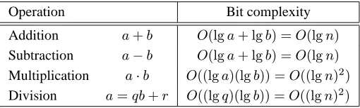
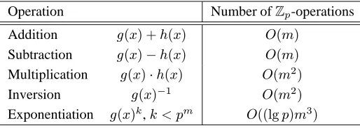
Letaandbbe non-negative integers, each less than or equal ton. Recall (Example 2.51) that the number of bits in the binary representation ofnis⌊lgn⌋+ 1, and this number is approximated bylgn. The number of bit operations for the four basic integer operations of addition, subtraction, multiplication, and division using the classical algorithms is summa-rized in Table 2.1. These algorithms are studied in more detail in§14.2. More sophisticated techniques for multiplication and division have smaller complexities.
Operation Bit complexity
Addition a+b O(lga+ lgb) =O(lgn)
Subtraction a−b O(lga+ lgb) =O(lgn)
Multiplication a·b O((lga)(lgb)) =O((lgn)2)
Division a=qb+r O((lgq)(lgb)) =O((lgn)2)
Table 2.1:Bit complexity of basic operations inZ.
The greatest common divisor of two integersaandbcan be computed via Fact 2.98. However, computing a gcd by first obtaining prime-power factorizations does not result in an efficient algorithm, as the problem of factoring integers appears to be relatively diffi-cult. The Euclidean algorithm (Algorithm 2.104) is an efficient algorithm for computing the greatest common divisor of two integers that does not require the factorization of the integers. It is based on the following simple fact.
2.103 Fact Ifaandbare positive integers witha > b, thengcd(a, b) = gcd(b, amodb).
2.104 AlgorithmEuclidean algorithm for computing the greatest common divisor of two integers
INPUT: two non-negative integersaandbwitha≥b. OUTPUT: the greatest common divisor ofaandb.
1. Whileb6= 0do the following: 1.1 Setr←amodb, a←b, b←r. 2. Return(a).
2.105 Fact Algorithm 2.104 has a running time ofO((lgn)2)bit operations.
2.106 Example (Euclidean algorithm) The following are the division steps of Algorithm 2.104 for computinggcd(4864,3458) = 38:
4864 = 1·3458 + 1406 3458 = 2·1406 + 646 1406 = 2·646 + 114
646 = 5·114 + 76 114 = 1·76 + 38
The Euclidean algorithm can be extended so that it not only yields the greatest common divisordof two integersaandb, but also integersxandysatisfyingax+by=d.
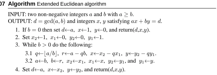
2.107 AlgorithmExtended Euclidean algorithm
INPUT: two non-negative integersaandbwitha≥b.
OUTPUT:d= gcd(a, b)and integersx,ysatisfyingax+by=d. 1. Ifb= 0then setd←a, x←1, y←0, and return(d,x,y). 2. Setx2←1, x1←0, y2←0, y1←1.
3. Whileb >0do the following:
3.1 q←⌊a/b⌋, r←a−qb, x←x2−qx1, y←y2−qy1.
3.2 a←b, b←r, x2←x1, x1←x, y2←y1, and y1←y.
4. Setd←a, x←x2, y←y2, and return(d,x,y).
2.108 Fact Algorithm 2.107 has a running time ofO((lgn)2)bit operations.
2.109 Example (extended Euclidean algorithm) Table 2.2 shows the steps of Algorithm 2.107 with inputsa = 4864andb = 3458. Hencegcd(4864,3458) = 38and(4864)(32) +
(3458)(−45) = 38.
q r x y a b x2 x1 y2 y1
− − − − 4864 3458 1 0 0 1
1 1406 1 −1 3458 1406 0 1 1 −1
2 646 −2 3 1406 646 1 −2 −1 3
2 114 5 −7 646 114 −2 5 3 −7
5 76 −27 38 114 76 5 −27 −7 38 1 38 32 −45 76 38 −27 32 38 −45 2 0 −91 128 38 0 32 −91 −45 128
Table 2.2:Extended Euclidean algorithm (Algorithm 2.107) with inputsa= 4864,b= 3458. Efficient algorithms for gcd and extended gcd computations are further studied in§14.4.
2.4.3 The integers modulo
n
Letnbe a positive integer.
2.110 Definition Ifaandbare integers, thenais said to be congruent tobmodulon, written
a≡b (modn), ifndivides(a−b). The integernis called the modulus of the congruence.
2.111 Example (i)24≡9 (mod 5)since24−9 = 3·5.
(ii)−11≡17 (mod 7)since−11−17 =−4·7.
2.112 Fact (properties of congruences) For alla,a1,b,b1,c∈Z, the following are true.
(i) a≡b (modn)if and only ifaandbleave the same remainder when divided byn. (ii) (reflexivity)a≡a (mod n).
(iv) (transitivity) Ifa≡b (modn)andb≡c (modn), thena≡c (modn).
(v) Ifa ≡ a1 (modn)andb ≡ b1 (modn), thena+b ≡ a1 +b1 (modn)and ab≡a1b1 (mod n).
The equivalence class of an integerais the set of all integers congruent toamodulo
n. From properties (ii), (iii), and (iv) above, it can be seen that for a fixednthe relation of congruence modulonpartitionsZinto equivalence classes. Now, ifa = qn+r, where
0≤r < n, thena≡r (mod n). Hence each integerais congruent modulonto a unique integer between0andn−1, called the least residue ofamodulon. Thusaandrare in the same equivalence class, and sormay simply be used to represent this equivalence class.
2.113 Definition The integers modulon, denotedZn, is the set of (equivalence classes of) in-tegers{0,1,2, . . . , n−1}. Addition, subtraction, and multiplication inZnare performed modulon.
2.114 Example Z25 = {0,1,2, . . . ,24}. InZ25,13 + 16 = 4, since13 + 16 = 29 ≡ 4
(mod 25). Similarly,13·16 = 8inZ25.
2.115 Definition Leta ∈ Zn. The multiplicative inverse ofamodulonis an integerx ∈Zn
such thatax≡1 (modn). If such anxexists, then it is unique, andais said to be
invert-ible, or a unit; the inverse ofais denoted bya−1.
2.116 Definition Leta, b∈Zn. Division ofabybmodulonis the product ofaandb−1modulo n, and is only defined ifbis invertible modulon.
2.117 Fact Leta∈Zn. Thenais invertible if and only ifgcd(a, n) = 1.
2.118 Example The invertible elements inZ9 are1,2,4,5,7, and8. For example,4−1 = 7
because4·7≡1 (mod 9).
The following is a generalization of Fact 2.117.
2.119 Fact Letd= gcd(a, n). The congruence equationax≡ b (modn)has a solutionxif and only ifddividesb, in which case there are exactlydsolutions between0andn−1; these solutions are all congruent modulon/d.
2.120 Fact (Chinese remainder theorem, CRT) If the integersn1, n2, . . . , nkare pairwise
rela-tively prime, then the system of simultaneous congruences
x ≡ a1 (mod n1) x ≡ a2 (mod n2)
.. .
x ≡ ak (modnk)
has a unique solution modulon=n1n2· · ·nk.
2.121 Algorithm (Gauss’s algorithm) The solutionxto the simultaneous congruences in the Chinese remainder theorem (Fact 2.120) may be computed asx=Pki=1aiNiMimodn,
whereNi = n/ni andMi = Ni−1modni. These computations can be performed in
Another efficient practical algorithm for solving simultaneous congruences in the Chinese remainder theorem is presented in§14.5.
2.122 Example The pair of congruencesx≡3 (mod 7),x≡7 (mod 13)has a unique
solu-tionx≡59 (mod 91).
2.123 Fact Ifgcd(n1, n2) = 1, then the pair of congruencesx≡a (mod n1),x≡a (modn2)
has a unique solutionx≡a (modn1n2).
2.124 Definition The multiplicative group ofZn isZ∗n = {a ∈ Zn | gcd(a, n) = 1}.In particular, ifnis a prime, thenZ∗n={a|1≤a≤n−1}.
2.125 Definition The order ofZ∗nis defined to be the number of elements inZ∗n, namely|Z∗n|. It follows from the definition of the Euler phi function (Definition 2.100) that|Z∗n|= φ(n). Note also that ifa ∈ Z∗nandb ∈ Z∗n, thena·b ∈ Z∗n, and soZ∗n is closed under multiplication.
2.126 Fact Letn≥2be an integer.
(i) (Euler’s theorem) Ifa∈Z∗n, thenaφ(n)≡1 (modn).
(ii) Ifnis a product of distinct primes, and ifr≡s (modφ(n)), thenar≡as (mod n)
for all integersa. In other words, when working modulo such ann, exponents can be reduced moduloφ(n).
A special case of Euler’s theorem is Fermat’s (little) theorem.
2.127 Fact Letpbe a prime.
(i) (Fermat’s theorem) Ifgcd(a, p) = 1, thenap−1≡1 (modp).
(ii) Ifr ≡ s (modp−1), thenar ≡ as (mod p)for all integersa. In other words,
when working modulo a primep, exponents can be reduced modulop−1. (iii) In particular,ap≡a (modp)for all integersa.
2.128 Definition Leta∈Z∗n. The order ofa, denotedord(a), is the least positive integertsuch thatat≡1 (modn).
2.129 Fact If the order ofa ∈ Z∗n ist, andas ≡ 1 (modn), thentdividess. In particular,
t|φ(n).
2.130 Example Letn = 21. ThenZ∗21 = {1,2,4,5,8,10,11,13,16,17,19,20}. Note that
φ(21) =φ(7)φ(3) = 12 =|Z∗21|. The orders of elements inZ∗21are listed in Table 2.3.
a∈Z∗21 1 2 4 5 8 10 11 13 16 17 19 20
order ofa 1 6 3 6 2 6 6 2 3 6 6 2
Table 2.3:Orders of elements inZ∗21.
2.131 Definition Letα ∈ Z∗n. If the order ofαisφ(n), thenαis said to be a generator or a
2.132 Fact (properties of generators ofZ∗n)
(i) Z∗nhas a generator if and only ifn = 2,4, pkor2pk, wherepis an odd prime and
k≥1. In particular, ifpis a prime, thenZ∗phas a generator.
(ii) Ifαis a generator ofZ∗n, thenZ∗n={αimodn|0≤i≤φ(n)−1}.
(iii) Suppose thatαis a generator ofZ∗n. Thenb =αi modnis also a generator ofZ∗
n
if and only ifgcd(i, φ(n)) = 1. It follows that ifZ∗nis cyclic, then the number of generators isφ(φ(n)).
(iv) α ∈ Z∗n is a generator ofZ∗nif and only ifαφ(n)/p 6≡ 1 (modn)for each prime
divisorpofφ(n).
2.133 Example Z∗21is not cyclic since it does not contain an element of orderφ(21) = 12(see Table 2.3); note that21does not satisfy the condition of Fact 2.132(i). On the other hand,
Z∗25is cyclic, and has a generatorα= 2.
2.134 Definition Leta∈Z∗n.ais said to be a quadratic residue modulon, or a square modulo
n, if there exists anx∈Z∗nsuch thatx2≡a (mod n). If no suchxexists, thenais called
a quadratic non-residue modulon. The set of all quadratic residues modulonis denoted byQnand the set of all quadratic non-residues is denoted byQn.
Note that by definition06∈Z∗n, whence06∈Qnand06∈Qn.
2.135 Fact Letpbe an odd prime and letαbe a generator ofZ∗p. Thena ∈ Z∗p is a quadratic residue modulopif and only ifa=αimodp, whereiis an even integer. It follows that
|Qp| = (p−1)/2and|Qp|= (p−1)/2; that is, half of the elements inZ∗pare quadratic
residues and the other half are quadratic non-residues.
2.136 Example α= 6is a generator ofZ∗13. The powers ofαare listed in the following table.
i 0 1 2 3 4 5 6 7 8 9 10 11
αimod 13 1 6 10 8 9 2 12 7 3 5 4 11
HenceQ13={1,3,4,9,10,12}andQ13={2,5,6,7,8,11}. 2.137 Fact Letnbe a product of two distinct odd primespandq,n = pq. Thena ∈ Z∗n is a quadratic residue modulonif and only ifa ∈ Qpanda ∈ Qq. It follows that|Qn| =
|Qp| · |Qq|= (p−1)(q−1)/4and|Qn|= 3(p−1)(q−1)/4.
2.138 Example Letn= 21. ThenQ21={1,4,16}andQ21={2,5,8,10,11,13,17,19,20}.
2.139 Definition Leta∈ Qn. Ifx∈Zn∗ satisfiesx2 ≡ a (mod n), thenxis called a square
root ofamodulon.
2.140 Fact (number of square roots)
(i) Ifpis an odd prime anda∈Qp, thenahas exactly two square roots modulop.
(ii) More generally, letn=pe1
1 pe
2
2 · · ·pe
k
k where thepiare distinct odd primes andei≥
1. Ifa∈Qn, thenahas precisely2kdistinct square roots modulon.
2.141 Example The square roots of12modulo37are7and30. The square roots of121modulo
2.4.4 Algorithms in
Z
nLetnbe a positive integer. As before, the elements ofZnwill be represented by the integers
{0,1,2, . . . , n−1}.
Observe that ifa, b∈Zn, then
(a+b) modn=
a+b, ifa+b < n, a+b−n, ifa+b≥n.
Hence modular addition (and subtraction) can be performed without the need of a long di-vision. Modular multiplication ofaandbmay be accomplished by simply multiplyinga
andbas integers, and then taking the remainder of the result after division byn. Inverses inZncan be computed using the extended Euclidean algorithm as next described.
2.142 AlgorithmComputing multiplicative inverses inZn INPUT:a∈Zn.
OUTPUT:a−1modn, provided that it exists.
1. Use the extended Euclidean algorithm (Algorithm 2.107) to find integersxandysuch thatax+ny=d, whered= gcd(a, n).
2. Ifd >1, thena−1modndoes not exist. Otherwise, return(x).
Modular exponentiation can be performed efficiently with the repeated square-and-multiply algorithm (Algorithm 2.143), which is crucial for many cryptographic protocols. One version of this algorithm is based on the following observation. Let the binary repre-sentation ofkbePti=0ki2i, where eachki ∈ {0,1}. Then
ak=
t
Y
i=0 aki2
i
= (a20)k0(a2 1
)k1
· · ·(a2t)kt
.
2.143 AlgorithmRepeated square-and-multiply algorithm for exponentiation inZn
INPUT:a∈Zn, and integer0≤k < nwhose binary representation isk=Pti=0ki2i.
OUTPUT:akmodn.
1. Setb←1. Ifk= 0then return(b). 2. SetA←a.
3. Ifk0= 1then setb←a.
4. Forifrom 1 totdo the following: 4.1 SetA←A2modn.
4.2 Ifki= 1then setb←A·bmodn.
5. Return(b).
2.144 Example (modular exponentiation) Table 2.4 shows the steps involved in the computation
of5596mod 1234 = 1013.
i 0 1 2 3 4 5 6 7 8 9
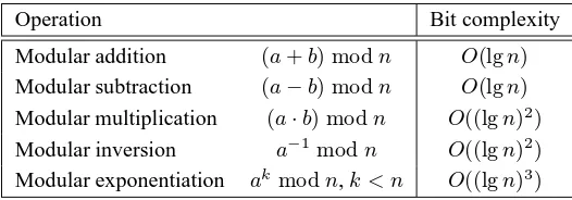
Table 2.5:Bit complexity of basic operations inZn.
2.4.5 The Legendre and Jacobi symbols
The Legendre symbol is a useful tool for keeping track of whether or not an integerais a quadratic residue modulo a primep.
2.145 Definition Letpbe an odd prime andaan integer. The Legendre symbol apis defined to be
2.146 Fact (properties of Legendre symbol) Letpbe an odd prime anda, b∈Z. Then the Leg-endre symbol has the following properties:
(v) (law of quadratic reciprocity) Ifqis an odd prime distinct fromp, then
p
2.147 Definition Letn≥3be odd with prime factorizationn=pe1
Observe that ifnis prime, then the Jacobi symbol is just the Legendre symbol.
2.148 Fact (properties of Jacobi symbol) Letm≥3,n≥3be odd integers, anda, b∈Z. Then the Jacobi symbol has the following properties:
(i) an= 0,1, or −1. Moreover, na= 0if and only ifgcd(a, n)6= 1.
By properties of the Jacobi symbol it follows that ifnis odd anda= 2ea
1wherea1
This observation yields the following recursive algorithm for computing an, which does not require the prime factorization ofn.
2.149 AlgorithmJacobi symbol (and Legendre symbol) computation
JACOBI(a,n)
INPUT: an odd integern≥3, and an integera,0≤a < n.
OUTPUT: the Jacobi symbol na(and hence the Legendre symbol whennis prime). 1. Ifa= 0then return(0).
2.151 Remark (finding quadratic non-residues modulo a primep) Letpdenote an odd prime. Even though it is known that half of the elements inZ∗pare quadratic non-residues modulo
p(see Fact 2.135), there is no deterministic polynomial-time algorithm known for finding one. A randomized algorithm for finding a quadratic non-residue is to simply select random integersa ∈Z∗puntil one is found satisfying ap =−1. The expected number iterations before a non-residue is found is2, and hence the procedure takes expected polynomial-time.
2.152 Example (Jacobi symbol computation) Fora= 158andn= 235, Algorithm 2.149 com-putes the Jacobi symbol 158235as follows:
Unlike the Legendre symbol, the Jacobi symbol andoes not reveal whether or nota
is a quadratic residue modulon. It is indeed true that ifa∈Qn, then an= 1. However, a
n
= 1does not imply thata∈Qn.
2.153 Example (quadratic residues and non-residues) Table 2.6 lists the elements inZ∗21and their Jacobi symbols. Recall from Example 2.138 thatQ21 = {1,4,16}. Observe that
Table 2.6:Jacobi symbols of elements inZ∗21.
2.154 Definition Letn≥ 3be an odd integer, and letJn ={a ∈Z∗n | na
2.156 Definition A Blum integer is a composite integer of the formn=pq, wherepandqare distinct primes each congruent to3modulo4.
2.157 Fact Letn = pqbe a Blum integer, and leta ∈ Qn. Thenahas precisely four square
roots modulon, exactly one of which is also inQn.
2.158 Definition Letnbe a Blum integer and leta∈Qn. The unique square root ofainQnis
2.159 Example (Blum integer) For the Blum integern = 21,Jn = {1,4,5,16,17,20}and
e
Qn={5,17,20}. The four square roots ofa= 4are2,5,16, and19, of which only16is
also inQ21. Thus16is the principal square root of4modulo21. 2.160 Fact Ifn= pqis a Blum integer, then the functionf : Qn −→ Qndefined byf(x) =
x2modnis a permutation. The inverse function off is: f−1(x) = x((p−1)(q−1)+4)/8modn.
2.5 Abstract algebra
This section provides an overview of basic algebraic objects and their properties, for refer-ence in the remainder of this handbook. Several of the definitions in§2.5.1 and§2.5.2 were presented earlier in§2.4.3 in the more concrete setting of the algebraic structureZ∗n.
2.161 Definition A binary operation∗on a setSis a mapping fromS×StoS. That is,∗is a rule which assigns to each ordered pair of elements fromSan element ofS.
2.5.1 Groups
2.162 Definition A group(G,∗)consists of a setGwith a binary operation∗onGsatisfying the following three axioms.
(i) The group operation is associative. That is,a∗(b∗c) = (a∗b)∗cfor alla, b, c∈G. (ii) There is an element1∈G, called the identity element, such thata∗1 = 1∗a=a
for alla∈G.
(iii) For eacha∈Gthere exists an elementa−1 ∈G, called the inverse ofa, such that a∗a−1=a−1∗a= 1.
A groupGis abelian (or commutative) if, furthermore, (iv) a∗b=b∗afor alla, b∈G.
Note that multiplicative group notation has been used for the group operation. If the group operation is addition, then the group is said to be an additive group, the identity ele-ment is denoted by0, and the inverse ofais denoted−a.
Henceforth, unless otherwise stated, the symbol∗will be omitted and the group oper-ation will simply be denoted by juxtaposition.
2.163 Definition A groupGis finite if|G|is finite. The number of elements in a finite group is called its order.
2.164 Example The set of integersZwith the operation of addition forms a group. The identity element is0and the inverse of an integerais the integer−a.
2.165 Example The setZn, with the operation of addition modulon, forms a group of order
2.166 Definition A non-empty subsetH of a groupGis a subgroup ofGifH is itself a group with respect to the operation ofG. IfH is a subgroup ofGandH 6=G, thenHis called a
proper subgroup ofG.
2.167 Definition A groupGis cyclic if there is an elementα∈Gsuch that for eachb∈Gthere is an integeriwithb=αi. Such an elementαis called a generator ofG.
2.168 Fact IfGis a group anda∈G, then the set of all powers ofaforms a cyclic subgroup of
G, called the subgroup generated bya, and denoted byhai.
2.169 Definition LetGbe a group anda∈G. The order ofais defined to be the least positive integertsuch thatat = 1, provided that such an integer exists. If such atdoes not exist,
then the order ofais defined to be∞.
2.170 Fact LetGbe a group, and leta∈Gbe an element of finite ordert. Then|hai|, the size of the subgroup generated bya, is equal tot.
2.171 Fact (Lagrange’s theorem) IfGis a finite group andHis a subgroup ofG, then|H|divides
|G|. Hence, ifa∈G, the order ofadivides|G|.
2.172 Fact Every subgroup of a cyclic groupGis also cyclic. In fact, ifGis a cyclic group of ordern, then for each positive divisordofn,Gcontains exactly one subgroup of orderd.
2.173 Fact LetGbe a group.
(i) If the order ofa∈Gist, then the order ofakist/gcd(t, k).
(ii) IfGis a cyclic group of ordernandd|n, thenGhas exactlyφ(d)elements of order
d. In particular,Ghasφ(n)generators.
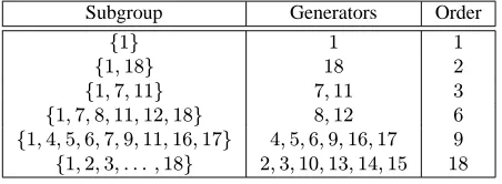
2.174 Example Consider the multiplicative groupZ∗19={1,2, . . . ,18}of order18. The group is cyclic (Fact 2.132(i)), and a generator isα= 2. The subgroups ofZ∗19, and their
gener-ators, are listed in Table 2.7.
Subgroup Generators Order
{1} 1 1
{1,18} 18 2
{1,7,11} 7,11 3
{1,7,8,11,12,18} 8,12 6
{1,4,5,6,7,9,11,16,17} 4,5,6,9,16,17 9
{1,2,3, . . . ,18} 2,3,10,13,14,15 18
Table 2.7:The subgroups ofZ∗19.
2.5.2 Rings
2.175 Definition A ring(R,+,×)consists of a setRwith two binary operations arbitrarily de-noted+(addition) and×(multiplication) onR, satisfying the following axioms.
(ii) The operation×is associative. That is,a×(b×c) = (a×b)×cfor alla, b, c∈R. (iii) There is a multiplicative identity denoted1, with16= 0, such that1×a=a×1 =a
for alla∈R.
(iv) The operation×is distributive over+. That is,a×(b+c) = (a×b) + (a×c)and
(b+c)×a= (b×a) + (c×a)for alla, b, c∈R. The ring is a commutative ring ifa×b=b×afor alla, b∈R.
2.176 Example The set of integersZwith the usual operations of addition and multiplication is
a commutative ring.
2.177 Example The setZnwith addition and multiplication performed modulonis a
commu-tative ring.
2.178 Definition An elementaof a ringRis called a unit or an invertible element if there is an elementb∈Rsuch thata×b= 1.
2.179 Fact The set of units in a ringRforms a group under multiplication, called the group of
units ofR.
2.180 Example The group of units of the ringZnisZ∗n(see Definition 2.124).
2.5.3 Fields
2.181 Definition A field is a commutative ring in which all non-zero elements have multiplica-tive inverses.
2.182 Definition The characteristic of a field is0if
mtimes
z }| {
1 + 1 +· · ·+ 1is never equal to0for any
m ≥1. Otherwise, the characteristic of the field is the least positive integermsuch that
Pm
i=11equals0.
2.183 Example The set of integers under the usual operations of addition and multiplication is not a field, since the only non-zero integers with multiplicative inverses are1and−1. How-ever, the rational numbersQ, the real numbersR, and the complex numbersCform fields of characteristic0under the usual operations.
2.184 Fact Znis a field (under the usual operations of addition and multiplication modulon) if
and only ifnis a prime number. Ifnis prime, thenZnhas characteristicn.
2.185 Fact If the characteristicmof a field is not0, thenmis a prime number.
2.5.4 Polynomial rings
2.187 Definition IfRis a commutative ring, then a polynomial in the indeterminatexover the ringRis an expression of the form
f(x) =anxn+· · ·+a2x2+a1x+a0
where eachai ∈ Randn ≥ 0. The elementai is called the coefficient ofxi inf(x).
The largest integermfor whicham 6= 0is called the degree off(x), denoteddegf(x);
amis called the leading coefficient off(x). Iff(x) = a0 (a constant polynomial) and a06= 0, thenf(x)has degree0. If all the coefficients off(x)are0, thenf(x)is called the zero polynomial and its degree, for mathematical convenience, is defined to be−∞. The polynomialf(x)is said to be monic if its leading coefficient is equal to1.
2.188 Definition IfRis a commutative ring, the polynomial ringR[x]is the ring formed by the set of all polynomials in the indeterminatexhaving coefficients fromR. The two opera-tions are the standard polynomial addition and multiplication, with coefficient arithmetic performed in the ringR.
2.189 Example (polynomial ring) Letf(x) =x3+x+ 1andg(x) =x2+xbe elements of
the polynomial ringZ2[x]. Working inZ2[x],
f(x) +g(x) =x3+x2+ 1
and
f(x)·g(x) =x5+x4+x3+x.
For the remainder of this section,Fwill denote an arbitrary field. The polynomial ring
F[x]has many properties in common with the integers (more precisely,F[x]andZare both
Euclidean domains, however, this generalization will not be pursued here). These
similar-ities are investigated further.
2.190 Definition Letf(x)∈F[x]be a polynomial of degree at least1. Thenf(x)is said to be
irreducible overF if it cannot be written as the product of two polynomials inF[x], each of positive degree.
2.191 Definition (division algorithm for polynomials) Ifg(x), h(x) ∈ F[x], withh(x) 6= 0, then ordinary polynomial long division ofg(x)byh(x)yields polynomialsq(x)andr(x)∈ F[x]such that
g(x) =q(x)h(x) +r(x), wheredegr(x)<degh(x).
Moreover,q(x)andr(x)are unique. The polynomialq(x)is called the quotient, while
r(x)is called the remainder. The remainder of the division is sometimes denotedg(x) mod h(x), and the quotient is sometimes denotedg(x) divh(x)(cf. Definition 2.82).
2.192 Example (polynomial division) Consider the polynomialsg(x) =x6+x5+x3+x2+x+1
andh(x) =x4+x3+ 1inZ
2[x]. Polynomial long division ofg(x)byh(x)yields g(x) =x2h(x) + (x3+x+ 1).