Machine Learning for Email
Drew Conway and John Myles White
Machine Learning for Email
by Drew Conway and John Myles White
Copyright © 2012 Drew Conway and John Myles White. All rights reserved. Printed in the United States of America.
Published by O’Reilly Media, Inc., 1005 Gravenstein Highway North, Sebastopol, CA 95472.
O’Reilly books may be purchased for educational, business, or sales promotional use. Online editions are also available for most titles (http://my.safaribooksonline.com). For more information, contact our corporate/institutional sales department: (800) 998-9938 or [email protected].
Editor: Julie Steele
Production Editor: Kristen Borg
Proofreader: O’Reilly Production Services
Cover Designer: Karen Montgomery
Interior Designer: David Futato
Illustrator: Robert Romano
Revision History for the First Edition:
2011-10-24 First release
See http://oreilly.com/catalog/errata.csp?isbn=9781449314309 for release details.
Nutshell Handbook, the Nutshell Handbook logo, and the O’Reilly logo are registered trademarks of O’Reilly Media, Inc. Machine Learning for Email, the image of an axolotl, and related trade dress are trademarks of O’Reilly Media, Inc.
Many of the designations used by manufacturers and sellers to distinguish their products are claimed as trademarks. Where those designations appear in this book, and O’Reilly Media, Inc., was aware of a trademark claim, the designations have been printed in caps or initial caps.
While every precaution has been taken in the preparation of this book, the publisher and authors assume no responsibility for errors or omissions, or for damages resulting from the use of the information con-tained herein.
ISBN: 978-1-449-31430-9
[LSI]
Table of Contents
Preface . . . vii
1. Using R . . . 1
R for Machine Learning 2
Downloading and Installing R 5
IDEs and Text Editors 8
Loading and Installing R Packages 9
R Basics for Machine Learning 11
Further Reading on R 26
2. Data Exploration . . . 29
Exploration vs. Confirmation 29
What is Data? 30
Inferring the Types of Columns in Your Data 34
Inferring Meaning 36
Numeric Summaries 37
Means, Medians, and Modes 37
Quantiles 40
Standard Deviations and Variances 41
Exploratory Data Visualization 43
Modes 54
Skewness 57
Thin Tails vs. Heavy Tails 59
Visualizing the Relationships between Columns 66
3. Classification: Spam Filtering . . . 75
This or That: Binary Classification 75
Moving Gently into Conditional Probability 80
Writing Our First Bayesian Spam Classifier 81
Defining the Classifier and Testing It with Hard Ham 88
Testing the Classifier Against All Email Types 91
Improving the Results 93
4. Ranking: Priority Inbox . . . 95
How Do You Sort Something When You Don’t Know the Order? 95
Ordering Email Messages by Priority 97
Priority Features Email 97
Writing a Priority Inbox 101
Functions for Extracting the Feature Set 102
Creating a Weighting Scheme for Ranking 109
Weighting from Email Thread Activity 115
Training and Testing the Ranker 119
Works Cited . . . 129
Preface
Machine Learning for Hackers: Email
To explain the perspective from which this book was written, it will be helpful to define the terms machine learning and hackers.
What is machine learning? At the highest level of abstraction, we can think of machine learning as a set of tools and methods that attempt to infer patterns and extract insight from a record of the observable world. For example, if we’re trying to teach a computer to recognize the zip codes written on the fronts of envelopes, our data may consist of photographs of the envelopes along with a record of the zip code that each envelope was addressed to. That is, within some context we can take a record of the actions of our subjects, learn from this record, and then create a model of these activities that will inform our understanding of this context going forward. In practice, this requires data, and in contemporary applications this often means a lot of data (several terabytes). Most machine learning techniques take the availability of such a data set as given— which, in light of the quantities of data that are produced in the course of running modern companies, means new opportunities.
What is a hacker? Far from the stylized depictions of nefarious teenagers or Gibsonian cyber-punks portrayed in pop culture, we believe a hacker is someone who likes to solve problems and experiment with new technologies. If you’ve ever sat down with the latest O’Reilly book on a new computer language and knuckled out code until you were well past “Hello, World,” then you’re a hacker. Or, if you’ve dismantled a new gadget until you understood the entire machinery’s architecture, then we probably mean you, too. These pursuits are often undertaken for no other reason than to have
gone through the process and gained some knowledge about the how and the why of
an unknown technology.
Along with an innate curiosity for how things work and a desire to build, a computer hacker (as opposed to a car hacker, life hacker, food hacker, etc.) has experience with software design and development. This is someone who has written programs before, likely in many different languages. To a hacker, UNIX is not a four-letter word, and command-line navigation and bash operations may come as naturally as working with
windowing operating systems. Using regular expressions and tools such as sed, awk and
grep are a hacker’s first line of defense when dealing with text. In the chapters of this
book, we will assume a relatively high level of this sort of knowledge.
How This Book is Organized
Machine learning exists at the intersection of traditional mathematics and statistics with software engineering and computer science. As such, there are many ways to learn the discipline. Considering its theoretical foundations in mathematics and statistics, newcomers would do well to attain some degree of mastery of the formal specifications of basic machine learning techniques. There are many excellent books that focus on
the fundamentals, the seminal work being Hastie, Tibshirani, and Friedman’s The
Elements of Statistical Learning [HTF09].* But another important part of the hacker mantra is to learn by doing. Many hackers may be more comfortable thinking of prob-lems in terms of the process by which a solution is attained, rather than the theoretical foundation from which the solution is derived.
From this perspective, an alternative approach to teaching machine learning would be to use “cookbook” style examples. To understand how a recommendation system works, for example, we might provide sample training data and a version of the model, and show how the latter uses the former. There are many useful texts of this kind as
well—Toby Segaran’s Programming Collective Intelligence is an recent example
[Seg07]. Such a discussion would certainly address the how of a hacker’s method of
learning, but perhaps less of the why. Along with understanding the mechanics of a
method, we may also want to learn why it is used in a certain context or to address a specific problem.
To provide a more complete reference on machine learning for hackers, therefore, we need to compromise between providing a deep review of the theoretical foundations of the discipline and a broad exploration of its applications. To accomplish this, we have decided to teach machine learning through selected case studies.
For that reason, each chapter of this book is a self-contained case study focusing on a specific problem in machine learning. The case studies in this book will focus on a single corpus of text data from email. This corpus will be used to explore techniques for classification and ranking of these messages.
*The Elements of Statistical Learning can now be downloaded free of charge at http://www-stat.stanford.edu/ ~tibs/ElemStatLearn/.
The primary tool we will use to explore these case studies is the R statistical program-ming language (http://www.r-project.org/). R is particularly well suited for machine learning case studies because it is a high-level, functional, scripting language designed for data analysis. Much of the underlying algorithmic scaffolding required is already built into the language, or has been implemented as one of the thousands of R packages
available on the Comprehensive R Archive Network (CRAN).† This will allow us to
focus on the how and the why of these problems, rather than reviewing and rewriting
the foundational code for each case.
Conventions Used in This Book
The following typographical conventions are used in this book:
Italic
Indicates new terms, URLs, email addresses, filenames, and file extensions.
Constant width
Used for program listings, as well as within paragraphs to refer to program elements such as variable or function names, databases, data types, environment variables, statements, and keywords.
Constant width bold
Shows commands or other text that should be typed literally by the user.
Constant width italic
Shows text that should be replaced with user-supplied values or by values deter-mined by context.
This icon signifies a tip, suggestion, or general note.
This icon indicates a warning or caution.
Using Code Examples
This book is here to help you get your job done. In general, you may use the code in this book in your programs and documentation. You do not need to contact us for permission unless you’re reproducing a significant portion of the code. For example, writing a program that uses several chunks of code from this book does not require
† For more information on CRAN, see http://cran.r-project.org/.
permission. Selling or distributing a CD-ROM of examples from O’Reilly books does require permission. Answering a question by citing this book and quoting example code does not require permission. Incorporating a significant amount of example code from this book into your product’s documentation does require permission.
We appreciate, but do not require, attribution. An attribution usually includes the title,
author, publisher, and ISBN. For example: “Machine Learning for Email by Drew
Con-way and John Myles White (O’Reilly). Copyright 2012 Drew ConCon-way and John Myles White, 978-1-449-31430-9.”
If you feel your use of code examples falls outside fair use or the permission given above, feel free to contact us at [email protected].
Safari® Books Online
Safari Books Online is an on-demand digital library that lets you easily search over 7,500 technology and creative reference books and videos to find the answers you need quickly.
With a subscription, you can read any page and watch any video from our library online. Read books on your cell phone and mobile devices. Access new titles before they are available for print, and get exclusive access to manuscripts in development and post feedback for the authors. Copy and paste code samples, organize your favorites, down-load chapters, bookmark key sections, create notes, print out pages, and benefit from tons of other time-saving features.
O’Reilly Media has uploaded this book to the Safari Books Online service. To have full digital access to this book and others on similar topics from O’Reilly and other pub-lishers, sign up for free at http://my.safaribooksonline.com.
How to Contact Us
Please address comments and questions concerning this book to the publisher: O’Reilly Media, Inc.
1005 Gravenstein Highway North Sebastopol, CA 95472
800-998-9938 (in the United States or Canada) 707-829-0515 (international or local)
707-829-0104 (fax)
We have a web page for this book, where we list errata, examples, and any additional information. You can access this page at:
http://oreilly.com/catalog/0636920022350
To comment or ask technical questions about this book, send email to:
For more information about our books, courses, conferences, and news, see our website at http://www.oreilly.com.
Find us on Facebook: http://facebook.com/oreilly
Follow us on Twitter: http://twitter.com/oreillymedia
Watch us on YouTube: http://www.youtube.com/oreillymedia
CHAPTER 1
Using R
Machine learning exists at the intersection of traditional mathematics and statistics with software engineering and computer science. In this book, we will describe several tools from traditional statistics that allow you to make sense of that world. Statistics has almost always been concerned with learning something interpretable from data, while machine learning has been concerned with turning data into something practical
and usable. This contrast makes it easier to understand the term machine learning:
Machine learning is concerned with teaching computers something about the world, so
that they can use that knowledge to perform other tasks, while statistics is more
con-cerned with developing tools for teaching humans something about the world, so that
they can think more clearly about the world in order to make better decisions.
In machine learning, the learning occurs by extracting as much information from the
data as possible (or reasonable) through algorithms that parse the basic structure of the data and distinguish the signal from the noise. After they have found the signal, or
pattern, the algorithms simply decide that everything else that’s left over is noise. For that reason, machine learning techniques are also referred to as pattern recognition algorithms. We can “train” our machines to learn about how data is generated in a given context, which allows us to use these algorithms to automate many useful tasks. This
is where the term training set comes from, referring to the set of data used to build a
machine learning process. The notion of observing data, learning from it, and then automating some process of recognition is at the heart of machine learning, and forms the primary arc of this book.
In this book, we will assume a relatively high degree of knowledge in basic programming techniques and algorithmic paradigms. That said, R remains a relatively niche language even among experienced programmers. In an effort to start everyone at the same start-ing point, this chapter will also provide some basic information on how to get started using the R language. Later in the chapter we will work through a specific example of using the R language to perform common tasks associated with machine learning.
This chapter does not provide a complete introduction to the R pro-gramming language. As you might expect, no such introduction could fit into a single book chapter. Instead, this chapter is meant to prepare the reader for the tasks associated with doing machine learning in R. Specifically, we describe the process of loading, exploring, cleaning, and analyzing data. There are many excellent resources on R that discuss language fundamentals; such as data types, arithmetic concepts, and coding best practices. Insofar as those topics are relevant to the case studies presented here, we will touch on all of these issues; however, there will be no explicit discussion of these topics. Some of these re-sources are listed in Table 1-1.
If you have never seen the language and its syntax before, we highly recommend going through this introduction to get some exposure. Unlike other high-level scripting lan-guages, such as Python or Ruby, R has a unique and somewhat prickly syntax and tends to have a steeper learning curve than other languages. If you have used R before, but not in the context of machine learning, there is still value in taking the time to go through this review before moving onto the cases.
R for Machine Learning
R is a language and environment for statistical computing and graphics...R provides a wide variety of statistical (linear and nonlinear modeling, classical statistical tests, time-series analysis, classification, clustering, ...) and graphical techniques, and is highly ex-tensible. The S language is often the vehicle of choice for research in statistical method-ology, and R provides an Open Source route to participation in that activity.
—The R Project for Statistical Computing, http://www.r-project.org/ The best thing about R is that it was developed by statisticians. The worst thing about R is that...it was developed by statisticians.
—Bo Cowgill, Google, Inc.
R is an extremely powerful language for manipulating and analyzing data. Its meteoric rise in popularity within the data science and machine learning communities has made it the de facto lingua franca for analytics. R’s success in the data analysis community stems from two factors described in the epitaphs above: R provides most of the technical power that statisticians require built into the default language, and R has been sup-ported by a community of statisticians who are also open source devotees.
There are many technical advantages afforded by a language designed specifically for statistical computing. As the description from the R Project notes, the language pro-vides an open-source bridge to S, which contains many highly-specialized statistical operations as base functions. For example, to perform a basic linear regression in R,
one must simply pass the data to the lm function, which then returns an object
con-taining detailed information about the regression (coefficients, standard errors, residual
values, etc.). This data can then be visualized by passing the results to the plot function,
which is designed to visualize the results of this analysis.
In other languages with large scientific computing communities, such as Python, du-plicating the functionality of lm requires the use of several third-party libraries to
rep-resent the data (NumPy), perform the analysis (SciPy) and visualize the results (matplotlib). As we will see in the following chapters, such sophisticated analyses can be performed with a single line of code in R.
In addition, as in other scientific computing environments, the fundamental data type in R is a vector. Vectors can be aggregated and organized in various ways, but at the core, all data are represented this way. This relatively rigid perspective on data struc-tures can be limiting, but is also logical given the application of the language. The most
frequently used data structure in R is the data frame, which can be thought of as a
matrix with attributes, an internally defined “spreadsheet” structure, or relational da-tabase-like structure in the core of the language. Fundamentally, a data frame is simply a column-wise aggregation of vectors that R affords specific functionality to, which makes it ideal for working with any manner of data.
For all of its power, R also has its disadvantages. R does not scale well with large data, and while there have been many efforts to address this problem, it remains a serious issue. For the purposes of the case studies we will review, however, this will not be an issue. The data sets we will use are relatively small, and all of the systems we will build are proto-types or proof-of-concept models. This distinction is important, be-cause if your intention is to build enterprise level machine learning sys-tems at the Google or Facebook scale, then R is not the right solution. In fact, companies like Google and Facebook often use R as their “data sandbox,” to play with data and experiment with new machine learning methods. If one of those experiments bears fruit, then the engineers will attempt to replicate the functionality designed in R in a more appropri-ate language, such as C.
This ethos of experimentation has also engendered a great sense of community around the language. The social advantages of R hinge on this large and growing community of experts using and contributing to the language. As Bo Cowgill alludes to, R was borne out of statisticians’ desire to have a computing environment that met their spe-cific needs. Many R users, therefore, are experts in their various fields. This includes an extremely diverse set of disciplines, including mathematics, statistics, biology, chemistry, physics, psychology, economics, and political science, to name a few. This community of experts has built a massive collection of packages on top of the extensive base functions in R. At the time of writing, CRAN contained over 2,800 packages. In the case studies that follow, we will use many of the most popular packages, but this will only scratch the surface of what is possible with R.
Finally, while the latter portion of Cowgill’s statement may seem a bit menacing, it further highlights the strength of the R community. As we will see, the R language has a particularly odd syntax that is rife with coding “gotchas” that can drive even experi-enced developers away. But all grammatical grievances with a language can eventually be overcome, especially for persistent hackers. What is more difficult for non-statisti-cians is the liberal assumption of familiarity with statistical and mathematical methods
built into R functions. Using the lm function as an example, if you had never performed
a linear regression, you would not know to look for coefficients, standard errors, or residual values in the results. Nor would you know how to interpret those results. But, because the language is open source, you are always able to look at the code of a function to see exactly what it is doing. Part of what we will attempt to accomplish with this book is to explore many of these functions in the context of machine learning, but that will ultimately only address a tiny subset of what you can do in R. Fortunately, the R community is full of people willing to help you understand not only the language, but also the methods implemented in it. Table 1-1 lists some of the best places to start.
Table 1-1. Community resources for R help
Resource Location Description
RSeek http://rseek.org/ When the core development team decided to create an open-source version of S and call it R, they had not considered how hard it would be to search for documents related to a single-letter language on the Web. This specialized search tool attempts to alleviate this by providing a focused portal to R documentation and information.
Official R mailing lists http://www.r-project.org/mail.html There are several listservs dedicated to the R lan-guage, including announcements, packages, de-velopment—and of course—help. Many of the language’s core developers frequent these lists, and responses are often quick and terse.
StackOverflow http://stackoverflow.com/questions/tagged/r Hackers will know StackOverflow.com as one of the premier web resources for coding tips in any language, and the R tag is no exception. Thanks to the efforts of several prominent R community members, there is an active and vibrant collec-tion of experts adding and answering R quescollec-tions on StackOverflow.
#rstats Twtter hash-tag http://search.twitter.com/search?q=%23rstats There is also a very active community of R users on Twitter, and they have adopted the #rstats hashtag as their signifier. The thread is a great place to find links to useful resources, find experts in the language, and post questions—as long as they can fit into 140 characters!
Resource Location Description
R-Bloggers http://www.r-bloggers.com/ There are hundreds of people blogging about how they use R in their research, work, or just for fun. R-bloggers.com aggregates these blogs and provides a single source for all things related to R in the blogosphere, and is a great place to learn by example.
Video Rchive http://www.vcasmo.com/user/drewconway As the R community grows, so too do the number of regional meetups and gatherings related to the language. The Rchive attempts to document the presentations and tutorials given at these meetings by posting videos and slides, and now contains presentations from community mem-bers all over the world.
The remainder of this chapter focuses on getting you set up with R and using it. This includes downloading and installing R, as well as installing R packages. We conclude with a miniature case study that will serve as an introduction to some of the R idioms we’ll use in later chapters. This includes issues of loading, cleaning, organizing, and analyzing data.
Downloading and Installing R
Like many open source projects, R is distributed by a series of regional mirrors. If you do not have R already installed on your machine, the first step is to download it. Go to
http://cran.r-project.org/mirrors.html and select the CRAN mirror closest to you. Once you have selected a mirror, you will need to download the appropriate distribution of R for whichever operating system you are running.
R relies on several legacy libraries compiled from C and Fortran. As such, depending on your operating system and your familiarity with installing software from source code, you may choose whether to install R from a compiled binary distribution or the source. Below, we present instruction for installing R on Windows, Mac OS X, and Linux distributions, with notes on installing from either source or binaries when available.
Finally, R is available in both 32- and 64-bit versions and, depending on your hardware and operating system combination, you should install the appropriate version.
Windows
For Windows operating systems there are two subdirectories available to install R:
base and contrib. The latter is a directory of compiled Windows binary versions of the
all of the contributed R packages in CRAN, while the former is the basic installation.
Select the base installation, and download the latest compiled binary. Installing
con-tributed packages is easy to do from R itself and is not language-specific; therefore, it
is not necessary to to install anything from the contrib directory. Follow the on-screen
instructions for the installation.
Once the installation has successfully completed, you will have an R application in your
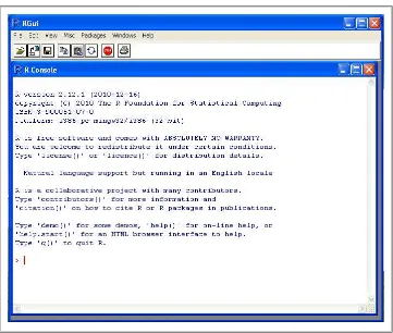
Start menu, which will open the RGui and R Console, as pictured in Figure 1-1.
Figure 1-1. The RGui and R console on a Windows installation
For most standard Windows installations, this process should proceed without any issues. If you have a customized installation, or encounter errors during the installation,
consult the R for Windows FAQ at your mirror of choice.
Mac OS X
Fortunately for Mac OS X users, R comes pre-installed with the operating system. You
can check this by opening the Terminal.app and simply typing R at the command-line.
You are now ready to begin! For some users, however, it will be useful to have a GUI application to interact with the R console. For this you will need to install separate software. With Mac OS X, you have the option of installing from either a compiled binary or the source. To install from a binary—recommended for users with no
experience using a Linux command line—simply download the latest version at your
mirror of choice at http://cran.r-project.org/mirrors.html and following the on-screen
instructions. Once the installation is complete, you will have both R.app (32-bit) and
R64.app (64-bit) available in your Applications folder. Depending on your version of Mac OS X and your machine’s hardware, you may choose which version you wish to work with.
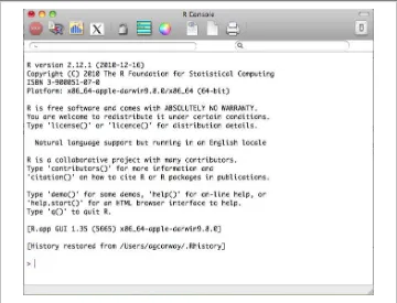
As with the Windows installation, if you are installing from binary this process should proceed without any problems. When you open your new R application you will see a console similar to the one pictured in Figure 1-2.
Figure 1-2. The R console on a 64-bit version of the Mac OS X installation
If you have a custom installation of Mac OS X or wish to customize the installation of R for your particular configuration, we recommend that you install from the source code. To install R from source on Mac OS X requires both C and Fortran compilers, which are not included in the standard installation of the operating system. You can install these compilers using the Mac OS X Developers Tools DVD included with your original Mac OS X installation package, or you can install the nec-essary compilers from the tools directory at the mirror of your choice.
Once you have all of the necessary compilers to install from source, the process is the typical configure, make, and install procedure used to install most software at the
command line. Using the Terminal.app, navigate to the folder with the source code and
execute the following commands:
$ ./configure $ make $ make install
Depending on your permission settings, you may have to invoke the sudo command as
a prefix to the configuration step and provide your system password. If you encounter any errors during the installation, using either the compiled binary distribution or the
source code, consult the R for Mac OS X FAQ at the mirror of your choice.
Linux
As with Mac OS X, R comes preinstalled on many Linux distributions. Simply type R
at the command line and the R console will be loaded. You can now begin program-ming! The CRAN mirror also includes installations specific to several Linux distribu-tions, with instructions for installing R on Debian, RedHat, SUSE, and Ubuntu. If you use one of these installations, we recommend that you consult the instructions for your operating system, because there is considerable variance in the best practices between Linux distributions.
IDEs and Text Editors
R is a scripting language and therefore the majority of the work done in this book’s case studies will be done within a IDE or text editor, rather than directly inputted into the R console. As we will show in the next section, some tasks are well suited for the console, such as package installation, but primarily you will want to be working within the IDE or text editor of your choice.
For those running the GUI in either Windows or Mac OS X, there is a basic text editor
available from that application. By navigating to File→New Document from the menu
bar, or clicking on the blank document icon in the header of the window (highlighted in Figure 1-3), you will open a blank document in the text editor. As a hacker, you likely already have an IDE or text editor of choice, and we recommend that you use whichever environment you are most comfortable in for the case studies. There are simply too many options to enumerate here, and we have no intention of inserting ourselves in the infamous emacs versus vim debate.
Figure 1-3. Text editor icon in R GUI
Loading and Installing R Packages
There are many well-designed, maintained, and supported R packages related to ma-chine learning. Loading packages in R is very straightforward. There are two functions
to perform this: library and require. There are some subtle differences between the
two, but for the purposes of this book, the primary difference is that require will return
a Boolean (TRUE or FALSE) value, indicating whether the package is installed on the
machine after attempting to load it. As an example, below we use library to load spatstat but require for lda. By using the print function, we can see that we have
lda installed because a Boolean value of TRUE was returned after the package was loaded:
library(spatstat) print(require(lda)) [1] TRUE
If we did not have lda installed (i.e., FALSE was returned by require), then we would
need to install that package before proceeding.
If you are working with a fresh installation of R, then you will have to install a number of packages to complete all of the case studies in this book.
There are two ways to install packages in R; either with the GUI interface or with the
install.packages function from the console. Given the intended audience for this book,
we will be interacting with R exclusively from the console during the case studies, but it is worth pointing out how to use the GUI interface to install packages. From the menu
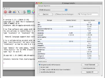
bar in the application, navigate to Packages &Data→Package Installer, and a window
will appear as displayed in Figure 1-4. From the Package Repository drop-down, select
either CRAN (binaries) or CRAN (sources) and click the Get List button to load all of the packages available for installation. The most recent version of packages will be
available in the CRAN (sources) repository, and if you have the necessary compilers
installed on your machine, we recommend using the sources repository. You can now select the package you wish to install and click Install Selected to install the packages.
Figure 1-4. Installing R packages using the GUI interface
The install.packages function is the preferred way to install packages because it pro-vides greater flexibility in how and where packages get installed. One of the primary
advantages of using install.packages is that it allows you to install from local source
code as well as from CRAN. Though uncommon, occasionally you may may want to install a package that is not yet available on CRAN—for example, if you’re updating to an experimental version of a package. In these cases you will need to install from source:
install.packages("tm", dependencies=TRUE) setwd("~/Downloads/")
install.packages("RCurl_1.5-0.tar.gz", repos=NULL, type="source")
In the first example above, we use the default settings to install the tm package from
CRAN. The tm provides function used to do text mining, and we will use it in
Chap-ter 3 to perform classification on email text. One useful parameter in the install.pack ages function is suggests, which by default is set to FALSE but if activated will instruct
the function to download and install any secondary packages used by the primary
in-stallation. As a best practice, we recommend always setting this to TRUE, especially if
you are working with a clean installation of R.
Alternatively, we can also install directly from compressed source files. In the example
above, we are installing the RCurl package from the source code available on the
au-thor’s website. Using the setwd function to make sure the R working directory is set to
the directory where the source file has been saved, we can simply execute the above command to install directly from the source code. Note the two parameters that have been altered in this case. First, we must tell the function not to use one of the CRAN
repositories by setting repos=NULL, and specify the type of installation using
type="source".
As mentioned, we will use several packages through the course of this text. Table 1-2
lists all of the packages used in the case studies and includes a brief description of their purpose, along with a link to additional information about each.
We are now ready to begin exploring machine learning with R! Before we proceed to the case studies, however, we will review some R functions and operations that we will use frequently.
Table 1-2. R packages used in this book
Name Location Author Description & Use
ggplot2 http://had.co .nz/ggplot2/
Hadley Wickham An implementation of the grammar of graphics in R. The premier pack-age for creating high-quality graphics.
plyr http://had.co .nz/plyr/
Hadley Wickham A set of tools used to manipulate, aggregate and manage data in R.
tm http://www .spatstat.org/ spatstat/
Ingo Feinerer A collection of functions for performing text mining in R. Used to work with unstructured text data.
R Basics for Machine Learning
UFO Sightings in the United States, from 1990-2010As we stated at the outset, we believe that the best way to learn a new technical skill is to start with a problem you wish to solve or a question you wish to answer. Being excited about the higher level vision of your work makes makes learning from case studies work. In this review of basic concepts in the R language, we will not be addressing a machine learning problem, but we will encounter several issues related to working with data and managing it in R. As we will see in the case studies, quite often we will spend the bulk of our time getting the data formatted and organized in a way that suits the analysis. Very little time, in terms of coding, is usually spent running the analysis. For this case we will address a question with pure entertainment value. Recently, the
data service Infochimps.com released a data set with over 60,000 documented reports
of unidentified flying objects (UFO) sightings. The data spans hundreds of years and has reports from all over the world. Though it is international, the majority of sightings in the data come from the United States. With the time and spatial dimensions of the data, one question we might ask is: are there seasonal trends in UFO sightings; and
what, if any, variation is there among UFO sightings across the different states in the U.S.?
This is a great data set to start exploring, because it is rich, well-structured, and fun to work with. It is also useful for this exercise because it is a large text file, which is typically the type of data we will deal with in this book. In such text files there are often messy parts, so we will use base functions in R and some external libraries to clean and or-ganize the raw data. This section will take you step-by-step through an entire simple analysis that tries to answer the questions we posed earlier. You will find the code for this section in the code folder for this chapter as the ufo_sightings.R file. We begin by
loading the data and required libraries for the analysis.
Loading libraries and the data
First, we will load the ggplot2 package, which we will use in the final steps of our visual analysis:
library(ggplot2)
While loading ggplot2, you will notice that this package also loads two other required
packages: plyr and reshape. Both of these packages are used for manipulating and
organizing data in R, and we will use plyr in this example to aggregate and organize
the data.
The next step is to load the data into R from the text file ufo_awesome.tsv, which is
located in data/ufo/ directory for this chapter. Note that the file is tab-delimited (hence
the .tsv file extension), which means we will need to use the read.delim function to
load the data. Because R exploits defaults very heavily, we have to be particularly con-scientious of the default parameter settings for the functions we use in our scripts. To see how we can learn about parameters in R, suppose that we had never used the
read.delim function before and needed to read the help files. Alternatively, assume that
we do not know that read.delim exists and need to find a function to read delimited
data into a data frame. R offers several useful functions for searching for help:
?read.delim # Access a function's help file
??base::delim # Search for 'delim' in all help files for functions # in 'base'
help.search("delimited") # Search for 'delimited' in all help files
RSiteSearch("parsing text") # Search for the term 'parsing text' on the R site.
In the first example, we append a question mark to the beginning of the function. This will open the help file for the given function and it’s an extremely useful R shortcut.
We can also search for specific terms inside of packages by using a combination of ??
and ::. The double question marks indicate a search for a specific term. In the example
above, we are searching for occurrences of the term “delim” in all base functions, using
the double colon. R also allows you to perform less structured help searches with
help.search and RSiteSearch. The help.search function will search all help files in your
installed packages for some term, which in the above example is “delimited.” Alterna-tively, you can search the R website, which includes help files and the mailing lists
archive, using the RSiteSearch function. Please note, this chapter is by no means meant
to be an exhaustive review of R or the functions used in this section. As such, we highly
recommend using these search functions to explore R’s base functions on your own.
For the UFO data there are several parameters in read.delim that we will need to set
by hand in order to properly read in the data. First, we need to tell the function how
the data are delimited. We know this is a tab-delimited file, so we set sep to the tab
character. Next, when read.delim is reading in data it attempts to convert each column
of data into an R data type using several heuristics. In our case, all of the columns are strings, but the default setting for all read.* functions is to convert strings to factor
types. This class is meant for categorical variables, but we do not want this. As such, we have to set stringsAsFactors=FALSE to prevent this. In fact, it is always a good prac-tice to switch off this default, especially when working with unfamiliar data.
The term “categorical variable” refers to a type of data that denotes an observation’s membership in a category. In statistics categorical varia-bles are very important because we may be interested in what makes certain observations belong to a certain type. In R we represent catego-rical variables as factor types, which essentially assigns numeric refer-ences to string labels. In this case, we convert certain strings—such as state abbreviations—into categorical variables using as.factor, which assigns a unique numeric ID to each state abbreviation in the data set. We will repeat this process many times.
Also, this data does not include a column header as its first row, so we will need to switch off that default as well to force R to not use the first row in the data as a header. Finally, there are many empty elements in the data, and we want to set those to the special R value NA. To do this we explicitly define the empty string as the na.string:
ufo<-read.delim("data/ufo/ufo_awesome.tsv", sep="\t", stringsAsFactors=FALSE, header=FALSE, na.strings="")
We now have a data frame containing all of the UFO data! Whenever working with data frames, especially if they are from external data sources, it is always a good idea to inspect the data by hand. Two great functions for doing this are head and tail. These
functions will print the first and last six entries in a data frame:
head(ufo) 6 19951025 19951024 Brunswick County, ND <NA> 30 min. Sheriff's office calls to re...
The first obvious issue with the data frame is that the column names are generic. Using the documentation for this data set as a reference, we can assign more meaningful labels to the columns. Having meaningful column names for data frames is an important best practice. It makes your code and output easier to understand, both for you and other
audiences. We will use the names function, which can either access the column labels
for a data structure or assign them. From the data documentation, we construct a character vector the corresponds to the appropriate column names and pass it to the
names functions with the data frame as its only argument:
names(ufo)<-c("DateOccurred","DateReported","Location","ShortDescription", "Duration","LongDescription")
From the head output and the documentation used to create column headings, we know
that the first two columns of data are dates. As in other languages, R treats dates as a special type, and we will want to convert the date strings to actual date types. To do
this we will use the as.Date function, which will take the date string and attempt to
convert it to as Date object. With this data the strings have an uncommon date format
of the form YYYYMMDD. As such, we will also have to specify a format string in
as.Date so the function knows how to convert the strings. We begin by converting the DateOccurred column:
ufo$DateOccurred<-as.Date(ufo$DateOccurred, format="%Y%m%d") Error in strptime(x, format, tz = "GMT") : input string is too long
We’ve just come upon our first error! Though a bit cryptic, the error message contains the substring “input string too long”, which indicates that some of the entries in the
DateOccurred column are too long to match the format string we provided. Why might
this be the case? We are dealing with a large text file, so perhaps some of the data was malformed in the original set. Assuming this is the case, those data points will not be
parsed correctly when being loaded by read.delim and that would cause this sort of
error. Because we are dealing with real world data, we’ll need to do some cleaning by hand.
Converting date strings, and dealing with malformed data
To address this problem we first need to locate the rows with defective date strings, then decide what to do with them. We are fortunate in this case because we know from the error that the errant entries are “too long.” Properly parsed strings will always be eight characters long, i.e., “YYYYMMDDD”. To find the problem rows, therefore, we simply need to find those that have strings with more than eight characters. As a best practice, we first inspect the data to see what the malformed data looks like, in order to get a better understanding of what has gone wrong. In this case, we will use the
head function, as before, to examine the data returned by our logical statement.
Later, to remove these errant rows we will use the ifelse function to construct a vector
of TRUE and FALSE values to identify the entries that are eight characters long (TRUE) and
those that are not (FALSE). This function is a vectorized version of the typical if-else
logical switch for some Boolean test. We will see many examples of vectorized opera-tions in R. They are the preferred mechanism for iterating over data because they are
often—but not always—more efficient:*
head(ufo[which(nchar(ufo$DateOccurred)!=8 | nchar(ufo$DateReported)!=8),1]) [1] "[email protected]"
[2] "0000"
[3] "Callers report sighting a number of soft white balls of lights headingin an easterly directing then changing direction to the west beforespeeding off to the north west."
[4] "0000" [5] "0000" [6] "0000"
good.rows<-ifelse(nchar(ufo$DateOccurred)>!=8 | nchar(ufo$DateReported)!=8, FALSE,TRUE)
length(which(!good.rows)) [1] 371
ufo<-ufo[good.rows,]
We use several useful R functions to perform this search. We need to know the length of the string in each entry of DateOccurred and DateReported, so we use the nchar
func-tion to compute this. If that length is not equal to eight, then we return FALSE. Once
we have the vectors of Booleans, we want to see how many entries in the data frame
have been malformed. To do this, we use the which command to return a vector of
vector indices that are FALSE. Next, we compute the length of that vector to find the
number of bad entries. With only 371 rows not conforming, the best option is to simply remove these entries and ignore them. At first, we might worry that losing 371 rows of data is a bad idea, but there are over sixty-thousand total rows, so we will simply ignore
those rows and continue with the conversion to Date types:
ufo$DateOccurred<-as.Date(ufo$DateOccurred, format="%Y%m%d") ufo$DateReported<-as.Date(ufo$DateReported, format="%Y%m%d")
Next we will need to clean and organize the location data. Recall from the previous
head call that the entries for UFO sightings in the United States take the form “City,
State”. We can use R’s regular expression integration to split these strings into separate columns and identify those entries that do not conform. The latter portion (identifying those that do not conform) is particularly important because we are only interested in sighting variation in the United States and will use this information to isolate those entries.
Organizing location data
To manipulate the data in this way, we will first construct a function that takes a string as input and performs the data cleaning. Then we will run this function over the location
data using one of the vectorized apply functions:
* For a brief introduction to vectorized operations in R see [LF08].
get.location<-function(l) {
split.location<-tryCatch(strsplit(l,",")[[1]], error= function(e) return(c(NA, NA))) clean.location<-gsub("^ ","",split.location)
There are several subtle things happening in this function. First, notice that we are
wrapping the strsplit command in R’s error handling function, tryCatch. Again, not
all of the entries are of the proper “City, State” form, and in fact some do not even
contain a comma. The strsplit function will throw an error if the split character is not
matched, therefore, we have to catch this error. In our case, when there is no comma to split we will return a vector of NA to indicate that this entry is not valid. Next, the
original data included leading whitespace, so we will use the gsub function (part of R’s
suite of functions for working with regular expressions) to remove the leading white-space from each character. Finally, we add an additional check to ensure that only the location vectors of length two are returned. Many non-U.S. entries have multiple com-mas, creating larger vectors from the strsplit function. In this case, we will again return
an NA vector.
With the function defined, we will use the lapply function, short for “list-apply,” to
iterate this function over all strings in the Location column. As mentioned, the apply
family of functions in R are extremely useful. They are constructed of the form
apply(vector, function), and return results of the vectorized application of the
func-tion to the vector in a specific form. In our case, we are using lapply, which always
From above, a list in R is a key-value style data structures, wherein the keys are indexed
by the double-bracket and values by the single bracket. In our case the keys are simply
integers, but lists can also have strings as keys.† Though convenient, having the data
stored in a list is not desirable, as we would like to add the city and state information to the data frame as separate columns. To do this we will need to convert this long list into a two-column matrix, with the city data as the leading column:
location.matrix<-do.call(rbind, city.state)
ufo<-transform(ufo, USCity=location.matrix[,1], USState=tolower(location.matrix[,2]), stringsAsFactors=FALSE)
To construct a matrix from the list, we use the do.call function. Similar to the apply functions, do.call executes a function call over a list. We will often use the
com-bination of lapply and do.call to manipulate data. Above we pass the rbind function,
which will “row-bind” all of the vectors in the city.state list to create a matrix. To get
this into the data frame we use the transform function. We create two new columns;
USCity and USState, from the first and second columns of location.matrix, respectively.
Finally, the state abbreviations are inconsistent, with some uppercase and others
lowercase, so we use the tolower function to make them all lowercase.
Dealing with data outside our scope
The final issue related to data cleaning we must consider concerns entries that meet the “City, State” form, but are not from the U.S. Specifically, the data include several UFO sightings from Canada, which also take this form. Fortunately, none of the Canadian province abbreviations match U.S. state abbreviations. We can use this information to identify non-U.S. entries by constructing a vector of U.S. state abbreviations and only
keeping those entries in the USState column that match an entry in this vector:
us.states<-c("ak","al","ar","az","ca","co","ct","de","fl","ga","hi","ia","id","il", "in","ks","ky","la","ma","md","me","mi","mn","mo","ms","mt","nc","nd","ne","nh", "nj","nm","nv","ny","oh","ok","or","pa","ri","sc","sd","tn","tx","ut","va","vt", "wa","wi","wv","wy")
ufo$USState<-us.states[match(ufo$USState,us.states)] ufo$USCity[is.na(ufo$USState)]<-NA
To find the entries in the USState column that do not match a U.S. state abbreviation,
we use the match function. This function takes two arguments: the first are the values
to be matched, and the second those to be matched against. What is returned is a vector of the same length as the first argument, in which the values are the index of entries in that vector that match some value in the second vector. If no match is found, the func-tion returns NA by default. In our case, we are only interested in which entries are NA,
as these are those entries that do not match a state. We then use the is.na function to
find which entries are not U.S. states and reset them to NA in the USState column. Finally, we also set those indices in the USCity column to NA for consistency.
† For a thorough introduction to lists, see Chapter 1 of [Spe08].
Our original data frame now has been manipulated to the point that we can extract from it only the data we are interested in. Specifically, we want a subset that includes only U.S. incidents of UFO sightings. By replacing entries that did not meet this criteria
in the previous steps, we can use the subset command to create a new data frame of
only U.S. incidents:
We now have our data in a format in which we can begin analyzing it! In the previous section we spent a lot of time getting the data properly formatted and identifying the relevant entries for our analysis. In this section we will explore the data to further narrow our focus. These data have two primary dimensions: space (where the sighting happened) and time (when a sighting occurred). We focused on the former in the
pre-vious section, but here we will focus on the latter. First, we use the summary function
on the DateOccurred column to get a sense of this chronological range of the data:
summary(ufo.us$DateOccurred)
Min. 1st Qu. Median Mean 3rd Qu. Max. "1400-06-30" "1999-09-06" "2004-01-10" "2001-02-13" "2007-07-26" "2010-08-30"
Surprisingly, this data goes back quite a long time:the oldest UFO sighting comes from 1400! Given this outlier, the next question is: how are these data distributed over time? And is it worth analyzing the entire time series? A quick way to look at this visually is to construct a histogram. We will discuss histograms in more detail in the next chapter, but for now you should know that histograms allow you to bin your data by a given dimension and observe the frequency with which your data falls into those bins. The dimension of interest here is time, so we construct a histogram that bins the data over time:
quick.hist<-ggplot(ufo.us, aes(x=DateOccurred))+geom_histogram()+ scale_x_date(major="50 years")
ggsave(plot=quick.hist, filename="../images/quick_hist.png", height=6, width=8) stat_bin: binwidth defaulted to range/30. Use 'binwidth = x' to adjust this.
There are several things to note here. This is our first use of the ggplot2 package, which
we will use throughout the book for all of our data visualizations. In this case, we are constructing a very simple histogram, which we only requires a single line of code. First,
we create a ggplot object and pass it the UFO data frame as its initial argument. Next,
we set the x-axis aesthetic to the DateOccurred column, as this is the frequency we are
interested in examining. With ggplot2 we must always work with data frames, and the
first argument to create a ggplot object must always be a data frame. ggplot2 is an R
implementation of Leland Wilkinson’s Grammar of Graphics [Wil05]. This means the
package adheres to this particular philosophy for data visualization, and all visualiza-tions will be built up as a series of layers. For this histogram, the initial layer is the x-axis data, namely the UFO sighting dates. Next, we add an histogram layer with the
geom_histogram function. In this case, we will use the default settings for this function,
but, as we will see later, this default is often not a good choice. Finally, because this data spans such a long time period, we will rescale the x-axis labels to occur every 50
years with the scale_x_date function.
Once the ggplot object has been constructed, we use the ggsave function to output the
visualization to a file. We could have also used > print(quick.hist) to print the
visu-alization to the screen. Note the warning message that is printed when you draw the visualization. There are many ways to bin data in a histogram, and we will discuss this in detail the next chapter, but this warning is provided to let you know exactly how
ggplot2 does the binning by default.
We are now ready to explore the data with this visualization, which is illustrated in
Figure 1-5.
The results of this analysis are stark. The vast majority of the data occur between 1960 and 2010, with the majority of UFO sightings occurring within the last two decades. For our purposes, therefore, we will focus on only those sightings that occurred between 1990 and 2010. This will allow us to exclude the outliers and compare relatively
com-parable units during the analysis. As before, we will used the subset function to create
a new data frame that meets this criteria:
ufo.us<-subset(ufo.us, DateOccurred>=as.Date("1990-01-01")) nrow(ufo.us)
[1] 46347
While this removes many more entries than we eliminated while cleaning the data, it still leaves us with over forty-six thousand observations to analyze. Next, we must begin organizing the data such that it can be used to address our central question: what, if any, seasonal variation exists for UFO sightings in U.S. states? To address this, we must first ask: what do we mean by “seasonal?” There are many ways to aggregate time series data with respect to seasons; by week, month, quarter, year, etc. But which way of
aggregating our data is most appropriate here? The DateOccurred column provides UFO
sighting information by the day, but there is considerable inconsistency in terms of the coverage throughout the entire set. We need to aggregate the data in a way that puts the amount of data for each state on relatively level planes. In this case, doing so by year-month is the best option. This aggregation also best addresses the core of our question, as monthly aggregation will give good insight into seasonal variations. We need to count the number of UFO sightings that occurred in each state by all year-month combinations from 1990-2010. First, we will need to create a new column in the data that corresponds to the year and months present in the data. We will use the
strftime function to convert the Date objects to a string of the “YYYY-MM” format.
As before, we will set the format parameter accordingly to get the strings:
ufo.us$YearMonth<-strftime(ufo.us$DateOccurred, format="%Y-%m")
Notice that in this case we did not use the transform function to add a new column to
the data frame. Rather, we simply referenced a column name that did not exists and R automatically added it. Both methods for adding new columns to a data frame are useful, and we will switch between them depending on the particular task. Next, we want to count the number of times each state and year-month combination occurs in the data. For the first time we will use the ddply function, which is part of the extremely
useful plyr library for manipulating data.
Figure 1-5. Exploratory histogram of UFO data over time
The plyr family of functions work a bit like the map-reduce style data aggregation tools
that have risen in popularity over the past several years. They attempt to group data in some specific way meaningful to all observations, and then do some calculation on each of these group and return the results. For this task we want to group the data by state abbreviations and the year-month column we just created. Once the data is grouped as such, we count the number of entries in each group and return that as a new column.
Here we will simply use the nrow function to reduce the data by the number of rows in
each group:
We now have the number of UFO sightings for each state by the year and month. From
the head call above, however, we can see that there may be a problem with using the
data as is, because it contains a lot of missing values. For example, we see that there was one UFO sighting in January, March, and May of 1990 in Arkansas; but no entries appear for February or April. Presumably, there were no UFO sightings in these months, but the data does not include entries for non-sightings, so we have to go back and add these as zeroes.
We need a vector of years and months that span the entire data set. From this we can check to see if they are already in the data, and if not, add them as zeroes. To do this,
we will create a sequence of dates using the seq.Date function, and then format them
to match the data in our data frame:
date.range<-seq.Date(from=as.Date(min(ufo.us$DateOccurred)), to=as.Date(max(ufo.us$DateOccurred)), by="month") date.strings<-strftime(date.range, "%Y-%m")
With the new date.strings vector, we need to create a new data frame that has all
year-months and states. We will use this to performing the matching with the UFO sighting data. As before, we will use the lapply function to create the columns and the do.call function to convert this to a matrix and then data frame:
states.dates<-lapply(us.states,function(s) cbind(s,date.strings))
The states.dates data frame now contains entries for every year, month and state
combination possible in the data. Note that there are now entries for February and April 1990 for Arkansas. To add in the missing zeroes to the UFO sighting data, we need to merge this data with our original data frame. To do this, we will use the
merge function, which takes two ordered data frames and attempts to merge them by
common columns. In our case, we have two data frames ordered alphabetically by U.S. state abbreviations and chronologically by year and month. We need to tell the function
which columns to merge these data frames by. We will set the by.x and by.y parameters
according to the matching column names in each data frame. Finally, we set the all
parameter to TRUE, which instructs the function to include entries that do not match
and fill them with NA. Those entries in the V1 column will be those state, year, and month
entries for which no UFOs were sighted:
all.sightings<-merge(states.dates,sightings.counts,by.x=c("s","date.strings"), by.y=c("USState","YearMonth"),all=TRUE)
head(all.sightings)
The final steps for data aggregation are simple housekeeping. First, we will set the
column names in the new all.sightings data frame to something meaningful. This is
done in exactly the same way as we did it at the outset. Next, we will convert the NA
entries to zeroes using the is.na function, again. Finally, we will convert the Year Month and State columns to the appropriate types. Using the date.range vector we
created in the previous step and the rep function to create a new vector that repeats a
given vector, we replace the year and month strings with the appropriate Date object.
Again, it is better to keep dates as Date objects rather than strings because we can
compare Date objects mathematically, but we can’t do that easily with strings. Likewise,
the state abbreviations are better represented as a categorical variables than strings, so
we convert these to factor types. We will describe factors, and other R data types, in
more detail in the next chapter:
names(all.sightings)<-c("State","YearMonth","Sightings") all.sightings$Sightings[is.na(all.sightings$Sightings)]<-0
all.sightings$YearMonth<-as.Date(rep(date.range,length(us.states))) all.sightings$State<-as.factor(toupper(all.sightings$State))
We are now ready to analyze the data visually!
Analyzing the data
For this data we will only address the core question by analyzing it visually. For the remainder of the book we will combine both numeric and visual analyses, but as this example is only meant to introduce core R programming paradigms, we will stop at the visual component. Unlike the previous histogram visualization, however, we will take greater care with ggplot2 to build the visual layers explicitly. This will allow us to
create a visualization that directly addresses the question of seasonal variation among states overtime and produce a more professional-looking visualization.
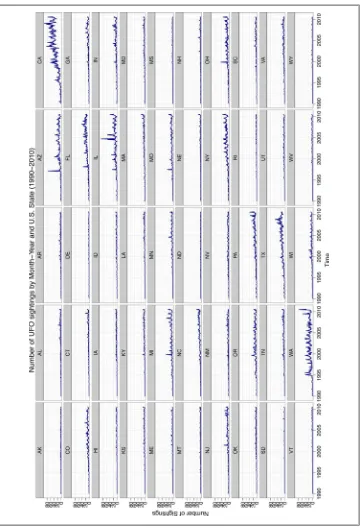
We will construct the visualization all at once below, then explain each layer individually:
state.plot<-ggplot(all.sightings, aes(x=YearMonth,y=Sightings)) +geom_line(aes(color="darkblue"))+
facet_wrap(~State,nrow=10,ncol=5)+ theme_bw()+
scale_color_manual(values=c("darkblue"="darkblue"),legend=FALSE)+ scale_x_date(major="5 years", format="%Y")+
xlab("Time")+ylab("Number of Sightings")+
opts(title="Number of UFO sightings by Month-Year and U.S. State (1990-2010)") ggsave(plot=state.plot, filename="../images/ufo_sightings.pdf",width=14,height=8.5)
As always, the first step is to create a ggplot object with a data frame as its first argument.
Here, we are using the all.sightings data frame we created in the previous step. Again,
we need to build an aesthetic layer of data to plot, and in this case the x-axis is the
YearMonth column and the y-axis is the Sightings data. Next, to show seasonal variation
among states, we will plot a line for each state. This will allow us to observe any spikes, lulls, or oscillation in the number of UFO sightings for each state over time. To do this,
we will use the geom_line function and set the color to “darkblue” to make the
visual-ization easier to read.
As we have seen throughout this case, the UFO data is fairly rich and includes many sightings across the United States over a long period of time. Knowing this, we need to think of a way to break up this visualization such that we can observe the data for each state, but also compare it to the others. If we plot all of the data in a single panel it will be very difficult to discern variation. To check this, run the first line of code from the above block, but replace color="darkblue" with color=State and enter > print(state.plot) at the console. A better approach would be to plot the data for each
state individually, and order them in a grid for easy comparison.
To create a multi-faceted plot, we use the facet_wrap function and specify that the
panels be created by the State variable, which is already a factor type, i.e., categorical.
We also explicitly define the number of rows and columns in the grid, which is easier in our case because we know we are creating 50 different plots.
The ggplot2 package has many plotting themes. The default theme is the one we used
in the first example and has a grey background with dark grey gridlines. While it is strictly a matter of taste, we prefer using a white background for this plot, since that