Model of Dynamic Pricing for Two Parallels Flights with
Multiple Fare Classes Based on Passenger Choice Behavior
Ahmad Rusdiansyah1, Dira Mariana2, Hilman Pradana3, Naning A. Wessiani4
Abstract: Airline revenue management (ARM) is one of emerging topics in transportation logistics areas. This paper discusses a problem in ARM which is dynamic pricing for two parallel flights owned by the same airline. We extended the existing model on Joint Pricing Model for Parallel Flights under passenger choice behavior in the literature. We generalized the model to consider multiple full-fare class instead of only single full-fare class. Consequently, we have to define the seat allocation for each fare class beforehand. We have combined the joint pricing model and the model of nested Expected Marginal Seat Revenue (EMSR) model. To solve this hybrid model, we have developed a dynamic programming-based algorithm. We also have conducted numerical experiments to show the behavior of our model. Our experiment results have showed that the expected revenue of both flights significantly induced by the proportion of the time flexible passengers and the number of allocated seat in each full-fare class. As managerial insights, our model has proved that there is a closed relationship between demand management, which is represented by the price of each fare class, and total expected revenue considering the passenger choice behavior.
Keywords: Airline revenue management, parallel flights, dynamic pricing, passanger choice behavior, seat allocation.
Introduction
Airline industry is one of service industry that applies revenue management. It has limited capacity and time of product service offerings. Specifically, tickets offered by airlines have characteristics such as perishable products. They have no residual value if passed a certain period. That is, if the tickets un-sold and the aircraft have to departure then revenue from unsold available seats will be lost.
Airline revenue management (ARM) is one of emerging topics in transportation logistics areas. The objective of ARM is to maximize passenger revenue by selling the right seats to the right customer at the right time (Dunleavy [4]). Airlines need to make decisions on “when” and “how many” ticket sold in high or low price to maximize the revenue.
In the literature, the models of ARM generally can be classified into two categories, static and dynamic models. The objective of the static model is to determine the number of seats that can be sold for each fare class.
1,2,3,4 Faculty of Industrial Technology, Transportation and
Distribution Logistics (TDLog) Research Group Logistics and Supply Chain Management Laboratory, Departement of Industrial Engineering, Institute Technology Sepuluh Nopember, Campus Keputih Sukolilo, Surabaya 60111. Email: [email protected]
Received 2nd February 2010; revised 26th April 2010. Accepted for publication 27th April 2010.
In other the number of seats that can be sold for each fare class. In other words, to limit the availability of seats in different booking classes or “booking limits”. In this model, the decision has been made before the selling process begins and it will not be adjusted during the entire booking period. A prominent literature discussing static models is Belobaba [2]. This approach is known Expected Mar-ginal Seat Revenue (EMSR). Some other papers are Smith et al. [7] and Weatherford and Bodily [10].
In the dynamic models, the booking control policy is not determined at the beginning of the booking period. The inventory seat allocation control should be dynamically reviewed over the entire booking period in order to optimize the expected revenue. Some papers discuss such problems including Lee and Hersh [6] and Subramanian, et al. [8] for discrete-time booking period and Feng and Xiao [5] for continuous-time booking model.
price but also some other preferences such as schedules, aircraft types and in-flight service. In the point of view passengers, the seat availability of multiple parallel flights can be substituted each other. To face this situation, the airline should manage demand well. When making adjustment ticket fares over the booking period, the airline should consider the choice behavior of passengers among different flights.
In general, based on their preference, there are two types of passengers; those travel for either business purposes or leisure purposes. The first group usually has strong time preferences. They tend to value booking or cancellation flexibility. They are relatively price-insensitive since, in most cases, their travel expenses are not by themselves. On the other hand, the second group, leisure passengers, tends to be more sensitive to price since they pay the tickets by their own budget (Tallury and van Ryzin, [9]).
Specifically, based on their choice behavior, some researchers have categorized passengers into some groups. Zang and Cooper [12] have classified them into two groups, high fare and low fare passengers. Moreover, in the context of two parallel flights (e.g. flight A and flight B), Xiao et al. [11] classified potential passengers into three types. Passengers’ type 1 and 2 are time-sensitive passengers. They buy only the ticket that is consistence with their departure-time requirements which are either flight A or flight B, respectively. They will never turn to buy the other flight even if lower price offered. In reality, most business travelers belong to this type. Passenger type 3 is price-sensitive passengers, which prefer to choose lower ticket price and do not consider the departure time. In reality, most leisure passengers belong to this type.
There are some papers discussing joint pricing for two parallel flights owned by the same airline. Zang and Cooper [12] proposed model in dynamic seat allocation control considering passenger choice behavior. Xiao et al. [11] also proposed dynamic pricing model for parallel flights problem. Moreover, Chen et al. [3] proposed model dynamic program-ming to optimize booking policy under seat allocation problem for two and multiple flight. However, none of these papers uses EMSR (Expected Marginal Seat Revenue) of Belobaba [2] which is commonly used in airline industry. We attempt to fulfill this research gap.
In our proposed model, we adopted EMSR approach to determine the seat allocation and booking level for each fare class in the cases of two parallel flights seat for a single-leg problem. We enhanced the EMSR model of Belobaba [2] to combine with the joint
dynamic pricing for parallel flights model of Xiao et al. [11]. The objective is to maximize total expected revenue of both flights by optimize seat allocation in each fare class.
First, we classified passengers into three types based on their choice behavior as of Xiao et al. [11]. We then determined seat allocation and booking level in each fare class using EMSR model. We finally applied dynamic programming to maximize the expected revenue of both flights.
Methods
Basic Models
Belobaba [2] developed nested EMSR approach model. This model is used to protect allocation seats of the higher fare level from the lower fare level. Using historical data, airlines can define demand level of each full-fare class. It is assumed that they have normal distribution with certain mean and standard deviation.
We adopted nested EMSR model to determine the seats allocation and booking level for each full-fare class. After defining the booking limits for each full-fare class, we then modified the model of Xiao et al. [11] on joint dynamic pricing to calculate the maximize expected total revenue of both flights. These two basic models will be explained in the next sub sections.
Seat Allocation Control Model of Belobaba[2]
There are two approaches to seat allocation problem, nested and non-nested allocations. Bazargan [1] has explained that in the nested allocation model, each fare class is assigned a booking limit. The booking limits are the total number of seats assigned to that fare class plus the sum of all seat allocations to its lower fare classes.
In non-nested model, distinct numbers of seats are exclusively assigned to each fare class. The sum of this allocation adds up to the total aircraft seat capacity. Figure 1 shows the visualization of these two approaches.
The EMSR method of Belobaba [2] generates the nested protection level for different class fare. This method proposed that in a nested seat allocation, the number of seats which should be protected for higher fare class i, over class j (lower class) is:
( )
( )
ji j i i i
j f P S f S
EMSR = . =
(1) The protected number of seats for the (n-1) fare class is determined by:
∑
=−−
=
Π
11 1
n
i i n
n
S
(2)
The average fare levels for the two classes of i and j are denote by fi and i
j jS
f . is the number of seats
that should be protected for higher class i over class j, thus
( )
ij iS
P is the probability of selling S or more
seats in fare class i.
The booking limit or the number of seat available for each class i, represented by BLi, is determined by
subtracting the number of seats protected for the higher fare class, Πi−1, from the total aircraft seat capacity, C. Therefore:
1
−
Π −
= i
i C
BL
(3) With the booking limit for the highest fare class is:
C
BL1= (4) The nested protection for fare class i is therefore the different between the booking limits for that fare and its lower fare class as follows:
1
+
−
= i i
i BL BL
NP (5)
Where NPi is the nested seat protection levels for
fare class i.
Joint Dynamic Pricing by Xiao, et al. [11]
In this section we will elaborate the model of Xiao et al. [11] as the main reference of our model. This model considers a situation where there are only two flights (flight A and B) owned by a same airline and scheduled at different times. The objective is to maximize the total revenue of both flights during the booking period [0,T].
As a nature of dynamic pricing, the ticket can be sold at k different prices. P is denoted as feasible price, in
which P = {p1,p2,…,pk} where p1 > p2 >…> pk. p1 is a
full price whereas pk is the lowest possible fare.
There are three types of passengers called Type I, Type II, Type III passengers, respectively. Type I (Type II) passengers select only flight A (or B), because they are time-sensitive passengers. Mean-while Type III passengers will choose the flight with a lower price.
The fractions of three passenger types are αi(∈ [0,1]),
i = 1,2,3, Σαi = 1 The potential passenger arrival
process follows Poisson with rate
λ
. Letλ
i =α
i.λ
, (i = 1, 2, 3) denotes the respective arrival rates of three types of passengers.The authors assumed that the choice behavior of passengers is only applied when the perceive value of passengers towards to the ticket is greater than the selling price. If the selling prices of both flights are higher than the perceive value, the passenger will not buy the ticket.
When the potential passenger arrived, they make a choice based on the current offered price by flight A and B (pA, pB). If passenger belong to type I or II,
then they will choose flight A or B if X≥pA, (X C pB). X is assume as the perceive value of each passenger. If Type III passengers then they will choose the flight with a lower price if X≥ (pA ΛpB). In case pA = pB and X≥pA, the passenger prefers choose flight A
with probability β(∈[0,1]) and prefers flight B with probability (1-β).
Thus, the probability of type I passenger to buy ticket flight A isF
( )
pA =1−F( )
pA ; the probability of type II passenger to buy ticket flight B is( )
pB F( )
pBF =1− ;. The probability of type III passenger to buy ticket either flight A or B is
(
pA pB)
F ∧ ; The effective arrival rates of flight A and B are then described as follows:
{ } { }
(
λ1+βλ3I pA=pB +λ2I pA<pB)
F(pA) and{ } { }
(
λ2+(1−β)λ3I pA=pB +λ3I pA<pB)
F(pB) (6) Where I{condition} is an indicator function with value 1 ifcondition is fulfilled, and 0 if otherwise.
This model assumes that the airline faces a Markov decision process. The airline seeks the minimization of the total expected revenue denoted by Rt(n1,n2),
over remaining horizon [t,T] where n1 (0≤n1≤C1) and n2 (0≤n2≤C2) represent the number of remaining
Supposed that the entire booking horizon [0,T] were divided into small intervals with equal length (Δt). Each of which will be called a period. It is assumed that there is no more than one passenger arrives over a period (Δt = 1). If λ represents the probability of arrival potential passenger in each period, thus, the value is 0 ≤λ≤ 1. At the same time, the potential passenger will buy based on their preference. If the passenger decides to buy a ticket, then the airline will collect the corresponding revenue and consume one unit of seat; otherwise the passenger losses.
The booking horizon [0,T] can be divided into two main general periods: period t < T and period T. Period T is defined the last period before the departure time. Since, the airline can only sell at most one unit of seat; thus, there may be remaining seats with no salvage value in the period T.
At the beginning of each period (in period t<T or in period T), the airline management needs to decide the optimal prices of the flights. The decision will be based on the forecasting of future demand and the current available seats.
Based on the number of available seat (n1,n2), there
are four cases considered as follows.
Case 1 if the tickets in both flights were sold out (n1 = n2 = 0).
Case 2 if flight A has sold out the ticket, and flight B have remaining seats (n1 = 0;
n2 > 0). The decision variable is flight B’s
selling price.
Case 3 if flight B has sold out the ticket while flight A have a number of unsold seats (n1 > 0; n2 = 0). The decision variable is
flight A’s selling price.
Case 4 if both tickets are still available
(n1 > 0, n2 > 0). A joint pricing decision is
required.
Enhanced Model
In this paper, we will explain our enhancement to the basic model of Xiao et al. [11]. Instead of only single full-fare class, we consider multiple full-fare class. Xiao et al. [11] only proposed model for an opened single fare class with k different prices, meanwhile we proposed m fare classes. Each of which, we consider k different prices.
Again, supposed that there two flights, A and B, are the parallel flights owned by the same airline company. It is assumed that that both flights have the same seat capacity (Ca = Cb). We also assume
that passengers are willing to pay more expensive when they booked the ticket lately. Thus, the airline
set m different full prices and the fare is higher if it is closed to the departure time.
For both flights, the airline set ma and mb full-fare
classes to open for flight A and B, respectively. Let ia
and ib be the indexes of opened class for flight A and
B respectively [(ia∈1..ma) and (ib∈1..mb)]. The
full-fare of flight A is represented by FFia and FFib
denotes full-fare of flight B.
Supposed that there are three full-fare classes for both flights (ma = mb = 3). Let FF1 be the highest
full-fare class and FF2be the lowest one. Thus, for both
flights, FF1 > FF2 > FF3.
For each full-fare class, we set k alternative prices. k is the number of different prices in each class iaand ib. Let P = {p1,p2,…,pk} be the set of alternative prices
where p1 is the full price and pk is the lowest possible
price. Without loss any generalization, we define that p1 > p2 >…> pk. If PiaA and PibB represent the price of class i opened in Flight A and B then A
ia
P =
(P x FFia) and PibB = (P x FFib).
The probability of type I passenger to buy ticket flight A in class ia is F
( )
PiaA =1−F( )
PiaA ; theprobability of type II passenger to buy ticket flight B in class ib is F
( )
PibB =1−F( )
PibB . The probability oftype III passenger to buy ticket flight A or B in class iaand ib isF
(
PiaA∧PibB)
.Thus, the effective arrival rates of flight A and B are as follows
Where I{condition} is an indicator function with value 1 if
Different from the single fare class model of Xiao et al. [11] where the seat allocation is a given para-meter, in multiple fare classes, we need to previously determine the seat allocation for each fare class. To solve this issue, we previously used the nested EMSR approach model of Belobaba [2]. The output of this model is the seat allocation for each class of Flight A and B. Similar to Xiao et al. [11], we also used backward dynamic program-ming to solve the problems.
Result and Discussion
Seat Allocation Control
We used the following parameter in the numerical experiments: There are 30 seats available f discount-ed prices (k=6). So the feasible set price is or each flight (Ca = Cb = 30 seats), and both flights opened 3
full-fare classes. For each of which, the ticket offered in a full price and five P = (1, 0.9, 0.8, 0.7, 0.6, 0.5). The probabilities that a potential passenger’s per-ceive value of above set selling price are (0.3, 0.4, 0.48, 0.58, 0.7 and 0.85) respectively. We have divided the entire horizon into T = 100, and the arrival rate of potential passenger is λ = 0.75.
We will discuss the model in three conditions. Condition 1:
In condition 1, we assume that the price of each classes is same for both flights; (FFia = FFib for all i),
and also under the same demand distribution. This means that Flight A and B have equal numbers of seat allocation in each fare class. It was sound un-realistic but we can use this condition in order to compare to other conditions. The details of para-meter in condition 1 are shown in Table 1.
Based on the nested EMSR approach, we determine seat allocation for each fare class. The seat allocation of each fare class is shown in Table 1. Figure 2 shows the visualization of EMSR for condition 1.
0 50 100 150 200 250 300
1 3 5 7 9 11 13 15 17 19 21 23 25 27 29
seats
FF1
FF2
FF3
EM
SR
Figure 2. EMSR for flights A and B in condition 1
Table 1. Parameter and seat allocation of the both flights for condition 1
Flight A & B
Capacity (seat) 30
Class (FFi) FF1 FF2 FF3
Fare ($) 250 200 150
Demand distribution Mean 8 10 12
SD 1.5 1.2 1
Seat allocation 7 10 13
Condition 2:
In condition 2, we assume that the prices of each class are same for both flights. However, they have different demand distribution. This means that Flight A and B have different number of seat allocation in each fare class. The parameter and seat allocation for this condition are shown in Table 2. We may see that seat allocation of flight A is similar to that of in condition 1
Condition 3:
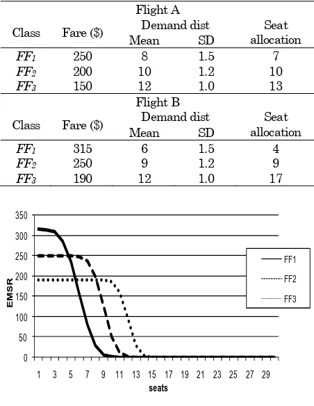
In condition 3, we assume the fares of each class in flight A and B are different. We assume that the price of flight B is more expensive than that of flight A. With different demand distribution, the seat allo-cation of each class can be seen in Table 3. The EMSR’s visualization for flight B is shown in Figure 4.
0 50 100 150 200 250 300
1 3 5 7 9 11 13 15 17 19 21 23 25 27 29
seats
FF1
FF2
FF3
EM
SR
Figure 3. EMSR for Flight B in condition 2
Table 2. Parameter and seat allocation of flight A & B for condition 2
Flight A
Class Fare ($) Demand dist Seat
allocation Mean SD
FF1 250 8 1.5 7
FF2 200 10 1.2 10
FF3 150 12 1.0 13
Flight B
Class Fare ($) Demand dist allocation Seat
Mean SD
FF1 250 6 1.5 4
FF2 200 10 1.2 10
Table 3. Parameter and seat allocation of flight A & B for condition 3
Flight A
Class Fare ($) Demand dist Seat
allocation Mean SD
FF1 250 8 1.5 7
FF2 200 10 1.2 10
FF3 150 12 1.0 13
Flight B
Class Fare ($) Demand dist Seat
allocation Mean SD
FF1 315 6 1.5 4
FF2 250 9 1.2 9
FF3 190 12 1.0 17
0 50 100 150 200 250 300 350
1 3 5 7 9 11 13 15 17 19 21 23 25 27 29
EMSR
seats
FF1
FF2
FF3
Figure 4. EMSR for Flight B in condition 3
Joint Pricing
After the seat allocation of each fare class has been determined, we then calculated the expected revenue of the joint flights under some different circum-stances. First, the numerical experiments using the different arrival rates of Type III passengers ( 3)
under the fixed probability of passengers prefer choosing flight A ( ).
Different Values of ǂ3
We computed the optimal total revenue under different values of 3 from 0 to 1 and keeping the ’s
value in 0.5. We set 1 = 2, so the values of 1 & 2
are equal to ( ) 2
1−α3 . The expected revenue of flights
is shown in Table 4, 5, and 6; respectively for Conditions 1, 2, and 3. We have compared the expected revenues of them. They are represented in Figure 5.
The results showed that proportion of type III passengers have influenced the total expected revenue of both flights. The higher value of 3, the
higher total expected revenue of joint flights. This implies that airline management needs to notice when inflexible time passengers become time flexible passengers, they need to manage the price of both flights in order to control their demand.
Table 4. The expected revenue of flights under different value of 3 in condition 1
Condition 1
3 1 = 2 Ra Rb Rtotal
0.0 0.50 2973.9165 2973.9165 5947.8330
0.1 0.45 2996.3259 2996.3259 5992.6519
0.2 0.40 3011.6638 3011.6638 6023.3276
0.3 0.35 3021.7126 3021.7126 6043.4253
0.4 0.30 3028.3787 3028.3809 6056.7595
0.5 0.25 3033.0530 3032.9888 6066.0417
0.6 0.20 3036.4031 3036.4031 6072.8062
0.7 0.15 3039.1101 3038.8000 6077.9102
0.8 0.10 3040.9736 3040.9563 6081.9299
0.9 0.05 3042.6343 3042.6558 6085.2900
Table 5. The expected revenue of flights under different value of 3 in condition 2
Condition 2
3 1 = 2 Ra Rb Rtotal
0.0 0.50 2973.917 2806.605 5780.522 0.1 0.45 2987.921 2835.062 5822.983 0.2 0.40 3002.359 2850.854 5853.214 0.3 0.35 3015.547 2858.305 5873.853 0.4 0.30 3029.331 2858.818 5888.149 0.5 0.25 3042.320 2856.173 5898.493 0.6 0.20 3055.663 2850.617 5906.279 0.7 0.15 3068.612 2843.718 5912.330 0.8 0.10 3081.812 2835.434 5917.245 0.9 0.05 3098.275 2823.265 5921.540
Table 6. The expected revenue of flights under different value of 3 in condition 3
Condition 3
3 1 = 2 Ra Rb Rtotal
0.0 0.50 2973.917 3500.278 6474.194
0.1 0.45 3050.730 3457.117 6507.846
0.2 0.40 3047.723 3493.441 6541.164
0.3 0.35 3020.185 3549.774 6569.959
0.4 0.30 2985.979 3607.504 6593.483
0.5 0.25 2953.355 3658.108 6611.463
0.6 0.20 2915.051 3709.565 6624.616
0.7 0.15 2889.885 3745.612 6635.497
0.8 0.10 2868.631 3776.945 6645.576
0.9 0.05 2840.368 3815.704 6656.072
5200 5400 5600 5800 6000 6200 6400 6600 6800
0 0.1 0.2 0.3 0.4 0.5 0.6 0.7 0.8 0.9
a3
condition 1 condition 2 condition 3
Figure 5. Total revenue in different value of 3
Rto
Specifically, by comparing the results of conditions 1 and 2, we may see that the total expected revenue of condition 1 is higher than that of condition 2. This is due to different demand distribution in each class of flights A and B.
We may make a conclusion that the seat allocation distribution of joint flights has significantly contri-buted to the total revenue received. Thus, in mana-gerial perspective, the airline management should optimize the seat allocation management of the joint flights. Our proposed model can be used for this purpose.
Different Values ofǃand Smallǂ3
We set values from 0 to 1, whereas 3 = 0.1, and 1 = 2 =0.45 are constant. We choose small proportion
for leisure passengers ( 3) to represent a condition
when time sensitive passengers are more dominant than price sensitive passengers. When selling prices of both flights are identical, the larger value of implies that type III passengers prefer choose flight A. As a result, for all conditions, the expected revenue of flight A increases.
The total expected revenue under different values of in condition 1 shown in Table 7 and Figure 6 has formed a curve shape. The highest revenue occurred when = 0.5, which is situation where both flights have identical price as well as the seat allocation.
Table 7. Rtotal under different value of in condition 1
Condition 1
Ra Rb Rtotal
0.0 2908.828 3082.3762 5991.2041 0.1 2925.605 3066.0991 5991.7043 0.2 2942.968 3049.1401 5992.1082 0.3 2960.701 3031.7056 5992.4063 0.4 2978.545 3014.0449 5992.5903 0.5 2996.326 2996.3259 5992.6519 0.6 3014.049 2978.5417 5992.5903 0.7 3031.706 2960.7007 5992.4063 0.8 3049.140 2942.9680 5992.1082 0.9 3066.101 2925.6030 5991.7041 1.0 3082.375 2908.8291 5991.2039
5990.0000 5990.5000 5991.0000 5991.5000 5992.0000 5992.5000 5993.0000
0 0.1 0.2 0.3 0.4 0.5 0.6 0.7 0.8 0.9 1
R
t
o
t
a
l
value of β
Figure 6. Total revenue in differentvalues of in condition 1
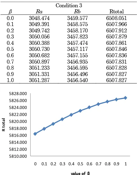
In condition 2, which is a situation when flights A and B have the same price but in different demand, the results showed that the higher the higher total expected revenue.
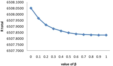
Different situation was occurred in condition 3. In this condition, we have set that the price of flight B is higher than that of flight A. The result is that the higher the lower total expected revenue.
These two experiments results imply that the airline will gain higher revenue if they set price of flight A higher than flight B, when the time flexible passenger prefers to choose flight A. Tables 8 and 9 represent total expected revenue of condition 2 and 3 under different values of . Figures 7 and 8 represent these two conditions in graphics respect-tively.
Table 8.Rtotal under different value of in condition 2
Condition 2
Ra Rb Rtotal
0.0 2912.733 2903.667 5816.400
0.1 2926.528 2891.314 5817.843
0.2 2940.864 2878.382 5819.245
0.3 2956.030 2864.555 5820.584
0.4 2971.646 2850.190 5821.836
0.5 2987.921 2835.062 5822.983
0.6 3004.570 2819.433 5824.003
0.7 3021.248 2803.638 5824.886
0.8 3037.945 2787.682 5825.627
0.9 3054.552 2771.668 5826.220
1.0 3071.302 2755.379 5826.682
Table 9. Rtotal under different value of in condition 3
Condition 3
Ra Rb Rtotal
0.0 3048.474 3459.577 6508.051
0.1 3049.391 3458.575 6507.966
0.2 3049.742 3458.170 6507.912
0.3 3050.056 3457.823 6507.879
0.4 3050.388 3457.474 6507.861
0.5 3050.730 3457.117 6507.846
0.6 3050.682 3457.155 6507.836
0.7 3050.897 3456.935 6507.831
0.8 3051.233 3456.595 6507.828
0.9 3051.331 3456.496 6507.827
1.0 3051.287 3456.540 6507.827
5810.000 5812.000 5814.000 5816.000 5818.000 5820.000 5822.000 5824.000 5826.000 5828.000
0 0.1 0.2 0.3 0.4 0.5 0.6 0.7 0.8 0.9 1
R
t
o
t
a
l
value of β
6507.7000 6507.7500 6507.8000 6507.8500 6507.9000 6507.9500 6508.0000 6508.0500 6508.1000
0 0.1 0.2 0.3 0.4 0.5 0.6 0.7 0.8 0.9 1
R
t
o
t
a
l
value of β
Figure 8. Total revenue in different values of in condition 3
Conclusion
In this paper, we have extended the model of Xiao et al. [11] of Joint Pricing Model for Parallel Flights. Instead of single full-fare class, we have considered the cases of multiple full-fare class. In this enhance-ment, we have employed the model of nested Expected Marginal Seat Revenue (EMSR) approach to previously define the seat allocation for each fare class. We have also modified the dynamic program-ming algorithm used by Xiao et al. [11]. Some numerical experiments have been conducted. Our experiment results has showed that the total expected revenue of both flights induced by propor-tion of time-flexible passengers (type III passengers) and the number of allocated seat in each full-fare class.
When the number of time-flexible passengers tends to increase, the airline has to set the price, in order to control the allocation of demand between two flights. The airline can gain higher revenue by set the price of full-fare class of one flight higher than another.
In general, we may conclude that our proposed model has shown that the closed relationships between demand management, which is represented by the price of each fare class, and total expected revenue considering the passenger choice behavior.
In this paper, we have not yet considered overbook-ing, cancellation and no show problems happened in reality condition. The future research of parallel flights problem can be considered in those situation.
References
1. Bazargan, M. Airline Operation and Scheduling. Ashgate. USA, 2004.
2. Belobaba, P. P., Air Travel Demand and Airline Seat Inventory Management, Ph.D. thesis, Flight Transportation Laboratory, Massachusetts Insti-tute of Technology, Cambridge, MA, 1987. 3. Chen, S., Gallego, G., Li, M. Z. F., and Lin, B. ,
Optimal Seat Allocation for Two Flight Problems with a Flexible Demand Segment, European Journal of Operation Research, 201(3), 2010, pp. 897-908.
4. Dunleavy, H., and Philips, G., The Future of Airline Revenue Management. Journal of Revenue Management, Vol. 8(4), 2009, pp.388-395.
5. Feng, Y, and Xiao, B., A Dynamic Airline Seat Inventory Control Model and Its Optimal Policy. Operation Research, 49(6), 2001, pp. 938-948. 6. Lee, T. C., and Hersh, M., A Model for Dynamic
Airline Seat Inventory Control with Multiple Seat Bookings. Transportation Science, 27, 1993, pp. 252–265.
7. Smith, B. C., Leimkuhler, J. F., and Darrow, R. M., Yield Management at American Airlines, Interfaces 22, 1992, pp. 8-31
8. Subramanian, J., Stidham, S., and Lautenbacher, C. J., Airlines Yield Management with Overbooking, Cancellation, and No-Shows. Transportation Science, 33(2), 1999, pp. 147-167. 9. Tallury, K. and van Ryzin, G. J., The Theory
and Practice of Revenue Management, Kluwer Academic Publisher, New York, 2007.
10. Weatherford, L. R.., and Bodily, S. E., A Taxonomy and Research Overview of Perishable Asset Revenue Management: Yield Management, Overbooking, and Pricing. Operations Research 40, 1992, pp. 831-834.
11. Xiao, Y. B., Chen, J., and Liu, X. L., Joint Dynamic Pricing for Two Parallel Flights based on Passenger Choice Behavior, System Engineering-Theory and Practice, 28(1), 2008, pp. 46-55.