Hidden semi-Markov models

(1)

Contents lists available atScienceDirect

Artiﬁcial Intelligence

www.elsevier.com/locate/artint

Hidden semi-Markov models

Shun-Zheng Yu

Department of Electronics and Communication Engineering, Sun Yat-Sen University, Guangzhou 510275, PR China

a r t i c l e

i n f o

a b s t r a c t

Article history: Received 14 April 2009

Available online 17 November 2009 Keywords:

Hidden Markov model (HMM) Hidden semi-Markov model (HSMM) Explicit duration HMM

Variable duration HMM Forward–backward (FB) algorithm Viterbi algorithm

As an extension to the popular hidden Markov model (HMM), a hidden semi-Markov model (HSMM) allows the underlying stochastic process to be a semi-Markov chain. Each state has variable duration and a number of observations being produced while in the state. This makes it suitable for use in a wider range of applications. Its forward– backward algorithms can be used to estimate/update the model parameters, determine the predicted, filtered and smoothed probabilities, evaluate goodness of an observation sequence fitting to the model, and find the best state sequence of the underlying stochastic process. Since the HSMM was initially introduced in 1980 for machine recognition of speech, it has been applied in thirty scientific and engineering areas, such as speech recognition/synthesis, human activity recognition/prediction, handwriting recognition, functional MRI brain mapping, and network anomaly detection. There are about three hundred papers published in the literature. An overview of HSMMs is presented in this paper, including modelling, inference, estimation, implementation and applications. It first provides a unified description of various HSMMs and discusses the general issues behind them. The boundary conditions of HSMM are extended. Then the conventional models, including the explicit duration, variable transition, and residential time of HSMM, are discussed. Various duration distributions and observation models are presented. Finally, the paper draws an outline of the applications.

1. Introduction (History)

A hidden Markov model (HMM) is defined as a doubly stochastic process. The underlying stochastic process is a discrete-time finite-state homogeneous Markov chain. The state sequence is not observable and so is called hidden. It influences another stochastic process that produces a sequence of observations. An excellent tutorial of HMMs can be found in Rabiner [150], a theoretic overview of HMMs can be found in Ephraim and Merhav [57] and a discussion on learning and inference in HMMs in understanding of Bayesian networks is presented in Ghahramani [66]. The HMMs are an important class of models that are successful in many application areas. However, due to the zero probability of self-transition of a non-absorbing state, the state duration of an HMM is implicitly a geometric distribution. This makes the HMM has limitations in some applications.

As an extension of the HMM, a hidden semi-Markov model (HSMM) is traditionally deﬁned by allowing the underlying process to be a semi-Markov chain. Each state has a variable duration, which is associated with the number of observations produced while in the state. The HSMM is also called “explicit duration HMM” [60,150], “variable-duration HMM” [107, 155,150], “HMM with explicit duration” [124], “hidden semi-Markov model” [126], generalized HMM [94], segmental HMM [157] and segment model [135,136] in the literature, depending on their assumptions and their application areas.

E-mail address:syu@mail.sysu.edu.cn.

(2)

The first approach to hidden semi-Markov model was proposed by Ferguson [60], which is partially included in the survey paper by Rabiner [150]. This approach is called the explicit duration HMM in contrast to the implicit duration of the HMM. It assumes that the state duration is generally distributed depending on the current state of the underlying semi-Markov process. It also assumes the “conditional independence” of outputs. Levinson [107] replaced the probability mass functions of duration with continuous probability density functions to form a continuously variable duration HMM. As Ferguson [60] pointed out, an HSMM can be realized in the HMM framework in which both the state and its sojourn time since entering the state are taken as a complex HMM state. This idea was exploited in 1991 by a 2-vector HMM [93] and a duration-dependent state transition model [179]. Since then, similar approaches were proposed in many applications. They are called in different names such as inhomogeneous HMM [151], non-stationary HMM [164], and recently triplet Markov chains [144]. These approaches, however, have the common problem of computational complexity in some applications. A more efficient algorithm was proposed in 2003 by Yu and Kobayashi [199], in which the forward–backward variables are defined using the notion of a state together with its remaining sojourn (or residual life) time. This makes the algorithm practical in many applications.

The HSMM has been successfully applied in many areas. The most successful application is in speech recognition. The ﬁrst application of HSMM in this area was made by Ferguson [60]. Since then, there have been more than one hundred such papers published in the literature. It is the application of HSMM in speech recognition that enriches the theory of HSMM and develops many algorithms for HSMM.

Since the beginning of 1990’s, the HSMM started being applied in many other areas such as electrocardiograph (ECG) [174], printed text recognition [4] or handwritten word recognition [95], recognition of human genes in DNA [94], language identiﬁcation [118], ground target tracking [88], document image comparison and classiﬁcation at the spatial layout level [81], etc.

In recent years from 2000 to present, the HSMM has been obtained more and more attentions from vast application areas such as change-point/end-point detection for semi-conductor manufacturing [64], protein structure prediction [162], mobility tracking in cellular networks [197], analysis of branching and flowering patterns in plants [69], rain events time se-ries model [159], brain functional MRI sequence analysis [58], satellite propagation channel modelling [112], Internet traffic modelling [198], event recognition in videos [79], speech synthesis [204,125], image segmentation [98], semantic learning for a mobile robot [167], anomaly detection for network security [201], symbolic plan recognition [54], terrain modelling [185], adaptive cumulative sum test for change detection in non-invasive mean blood pressure trend [193], equipment prognosis [14], financial time series modelling [22], remote sensing [147], classification of music [113], and prediction of particulate matter in the air [52], etc.

The rest of the paper is organized as follows: Section 2 is the major part of this paper that defines a unified HSMM and addresses important issues related to inference, estimation and implementation. Section 3 then presents three conventional HSMMs that are applied vastly in practice. Section 4 discusses the specific modelling issues, regarding duration distributions, observation distributions, variants of HSMMs, and the relationship to the conventional HMM. Finally, Section 5 highlights major applications of HSMMs and concludes the paper in Section 6.

2. Hidden semi-Markov model

This section provides a unified description of HSMMs. A general HSMM is defined without specific assumptions on the state transitions, duration distributions and observation distributions. Then the important issues related to inference, esti-mation and implementation of the HSMM are discussed. A general expression of the explicit-duration HMMs and segment HMMs can be found in Murphy [126], and a unified view of the segment HMMs can be found in Ostendorf et al. [136]. Detailed review for the conventional HMM can be found in the tutorial by Rabiner [150], the overview by Ephraim and Merhav [57], the Bayesian networks-based discussion by Ghahramani [66], and the book by Cappe et al. [29].

2.1. General model

A hidden semi-Markov model (HSMM) is an extension of HMM by allowing the underlying process to be a semi-Markov chain with a variableduration orsojourn time for each state. Therefore, in addition to the notation deﬁned for the HMM, the duration d of a given state is explicitly deﬁned for the HSMM. State duration is a random variable and assumes an integer value in the set

D

= {

1

,

2

, . . . ,

D

}

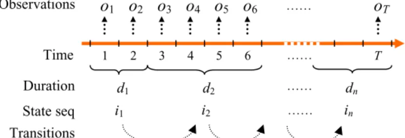
. The important difference between HMM and HSMM is that one observation per state is assumed in HMM while in HSMM each state can emit a sequence of observations. The number of observations produced while in stateiis determined by the length of time spent in statei, i.e., the durationd. Now we provide a uniﬁed description of HSMMs.

Assume a discrete-time Markov chain with the set of (hidden) states

S

= {

1

, . . . ,

M

}

. The state sequence is denoted by

S1:T

S1

, . . . ,

ST, where St

∈

S

is the state at timet. A realization ofS1:T is denoted ass1:T. For simplicity of notation in

the following sections, we denote:

•

St1:t2

=

i– stateithat the system stays in during the period fromt1tot2. In other words, it meansSt1

=

i,St1+1

=

i

, . . .

, andSt2

=

i. Note that the previous state St1−1 and the next stateSt2+1 may or may not bei.

(3)

Fig. 1.General HSMM.

•

S_[t1:t2]

=

i – stateiwhich starts at timet1 and ends att2 with durationd

=

t2

−

t1

+

1. This implies that the previous state St1−1and the next state St2+1must not bei.

•

S_[t1:t2

=

i – statei that starts at timet1 and lasts tillt2, with S[t1

=

i,St1+1

=

i

, . . .

, St2

=

i, where S[t1

=

i means that att1 the system switched from some other state toi, i.e., the previous statest1−1 must not bei. The next state St2+1 may or may not bei.

•

St1:t2]

=

i – statei that lasts fromt1tot2and ends att2withSt1

=

i, St1+1

=

i

, . . .

, St2]

=

i, where St2]

=

imeans that at timet2the state will end and transit to some other state, i.e., the next state St2+1must not bei. The previous state

St1−1may or may not bei.

Based on these deﬁnitions, S_[t]

=

imeans state istarting and ending att with duration 1,S_[t

=

i means statei starting

att,St]

=

imeans statei ending att, and St

=

imeans the state att being statei.

Denote the observation sequence by O1:T

O1

, . . . ,

OT, where Ot

∈

V

is the observable at time t and

V

=

{

v1

,

v2

, . . . ,

vK

}

is the set of observable values. For observation sequenceo1:T, the underlying state sequence isS1:d1]

=

i1,

S_[d1+1:d1+d2]

=

i2

, . . .

,S[d1+···+dn−1+1:d1+···+dn

=

in, and the state transitions are

(

im

,

dm

)

→

(

im+1

,

dm+1

)

, form

=

1

, . . . ,

n

−

1,

where

n_m₌₁dm

=

T, i1

, . . . ,

in

∈

S

, and d1

, . . . ,

dn

∈

D

. Note that the ﬁrst state i1 is not necessary starting at time 1

associated with the ﬁrst observation o1 and the last statein is not necessary ending at time T associated with the last

observation oT. Detailed discussion about the censoring issues can be found in Section 2.2.1. Deﬁne the state transition

probability from

(

i

,

d

)

→

(

j

,

d

)

fori

=

j by

a(i,d)(j,d)

P

[S

[t+1:t+d]

=

j|S[t−d+1:t]

=

i]

,

subject to

_j_∈_S_\{_i_}

_d_∈_Da(i,d)(j,d)

=

1 with zero self-transition probabilities a(i,d)(i,d)

=

0, where i

,

j

∈

S

and d

,

d

∈

D

. From the deﬁnition we can see that the previous state i started at t

−

d

+

1 and ended att, with duration d. Then it transits to state j having duration d, according to the state transition probabilitya(i,d)(j,d). State j will start att

+

1 and end att

+

d. This means both the state and the duration are dependent on both the previous state and its duration. While in state j, there will bedobservationsot+1:t+d being emitted. Denote this emission probability by

bj,d

(

ot+1:t+d

)

P

[

ot+1:t+d

|

S[t+1:t+d]

=

j

]

which is assumed to be independent to timet. Let the initial distribution of the state be

π

j,d

P

[

S[t−d+1:t]

=

j

]

,

t

0

,

d

∈

D.

It represents the probability of the initial state and its duration before timet

=

1 or before the ﬁrst observationo1obtained.

Then the set of the model parameters for the HSMM is deﬁned by

λ

a(i,d)(j,d)

,

bj,d

(

vk1:kd

),

π

i,d

,

wherei

,

j

∈

S

,d

,

d

∈

D

, andvk1:kd representsvk1

. . .

vkd

∈

V

× · · · ×

V

. This general HSMM is shown in Fig. 1.

The general HSMM is reduced to speciﬁc models of HSMM depending on the assumptions they made. For instance:

•

If the state duration is assumed to be independent to the previous state, then the state transition probability can be further speciﬁed asa(i,d)(j,d)

=

a(i,d)jpj

(

d

)

, where

(4)

is the transition probability from statei that has stayed for durationdto state jthat will start att

+

1, and

pj

(

d

)

P[St+1:t+d]

=

j|S[t+1

=

j] (2)

is the probability of durationdthat state jtakes. This is the model proposed by Marhasev et al. [119].

•

If a state transition is assumed to be independent to the duration of the previous state, then the state transition probability becomesa(i,d)(j,d)

=

ai(j,d), where

ai(j,d)

P

[

S[t+1:t+d]

=

j

|

St]

=

i

]

(3)

is the transition probability that statei ended att and transits to state j having durationd. This is the residential time HMM (see Section 3.3 for details). In this model, a state transition for i

=

j is

(

i

,

1

)

→

(

j

,

τ

)

and a self-transition is assumed to be

(

i

,

τ

)

→

(

i

,

τ

−

1

)

for

τ

>

1, where

τ

represents the residential time of the state.

•

If a self-transition is allowed and is assumed to be independent to the previous state, then the state transition proba-bility becomes a(i,d)(j,d)

=

a(i,d)j d

−1 τ=1 aj j

(

τ

)

1

−

aj j

(

d

)

,

whereaj j

(

d

)

P

[

St+d+1

=

j

|

S[t−d+1:t]

=

i

,

S_[t+1:t+d

=

j

] =

P

[

St+d+1

=

j

|

S[t+1:t+d

=

j

]

is the self-transition probability

when state jhas stayed fordtime units, and 1

−

aj j

(

d

)

=

P

[

St+d]

=

j

|

S[t+1:t+d

=

j

]

is the probability state j ends with

duration d. This is the variable transition HMM (see Section 3.2 for details). In this model, a state transition is either

(

i

,

d

)

→

(

j

,

1

)

fori

=

j or

(

i

,

d

)

→

(

i

,

d

+

1

)

for a self-transition.

•

If a transition to the current state is independent to the duration of the previous state and the duration is only condi-tioned on the current state, thena(i,d)(j,d)

=

ai jpj

(

d

)

, whereai j

P

[

S[t+1

=

j

|

St]

=

i

]

is the transition probability from state ito j, with the self-transition probabilityaii

=

0. This is the explicit duration HMM (see Section 3.1 for details).

Besides, the state duration distributions, pj

(

d

)

, can be parametric or non-parametric. The detailed discussion on various

duration distributions can be found in Section 4.1. Similarly, the observation distributionsbj,d

(

vk1:kd

)

can be parametric or

non-parametric, discrete or continuous, and dependent or independent on the state durations. It can also be a mixture of distributions. The detailed discussion on various observation distributions can be found in Section 4.2.

2.2. Inference

In this subsection we discuss the issues related to inference, including the forward–backward algorithm, calculation of probabilities and expectations, maximum a posteriori (MAP) estimate of states, maximum likelihood estimate (MLE) of state sequence, and constrained estimate of states.

2.2.1. The forward–backward algorithm

We deﬁne the forward variables for HSMM by:

α

t

(

j

,

d

)

P

[S

[t−d+1:t]

=

j

,

o1_:t

|

λ

]

and the backward variables by

β

t

(

j

,

d

)

P

[o

t+1:T

|S

[t−d+1:t]

=

j

, λ

]

.

Similar to deriving the formulas for the HMM (see e.g., Rabiner [150], Ephraim and Merhav [57]), it is easy to obtain the forward–backward algorithm for a general HSMM:

α

t

(

j

,

d

)

=

i∈S\{j}

d∈D

α

t−d i

,

d

·

a₍i,d)(j,d)

·

bj,d

(

ot−d+1:t

),

(4) fort

>

0

,

d

∈

D

,

j

∈

S

, and

β

t

(

j

,

d

)

=

i∈S\{j}

d∈D a(j,d)(i,d)

·

bi,d

(

ot+1:t+d

)

· β

t+d i

,

d

,

(5) fort

<

T.

The initial conditions generally can have two different assumptions:

•

The general assumption: assumes that the ﬁrst state begins at or before observationo1 and the last state ends at or after

observationoT. In this case, we can assume that the process starts at

−∞

and terminates at

+∞

. The observations out

(5)

formula (4) bj,d

(

ot−d+1:t

)

is replaced with the marginal distributionbj,d

(

o1:t

)

ift

−

d

+

1

1 and t

1, and in the

backward formula (5)bi,d

(

ot+1:t+d

)

is replaced with bi,d

(

ot+1:T

)

ift

+

1

T andt

+

d

T. We then have the initial

conditions for the forward recursion formula given by (4) as follows:

α

τ

(

j

,

d

)

=

P

[

S[τ−d+1:τ]

=

j

|

λ

] =

π

j,d

,

τ

0

,

d

∈

D,

where

{

π

j,d

}

can be the equilibrium distribution of the underlying semi-Markov process. Because, fort

+

d

T, P

[

S_[t+1:t+d]

=

i

,

ot+1:T

|

S[t−d+1:t]

=

j

, λ

] =

a(j,d)(i,d)bi,d otT+1

then from the backward recursion formula (5) we can see that

β

t+d

(

i

,

d

)

=

1, for t

+

d

T. Therefore, the initial

conditions for the backward recursion formula given by (5) are as follows:

β

τ

(

i

,

d

)

=

1

,

τ

T

,

d

∈

D.

If the model assumes that the ﬁrst state begins att

=

1 and the last state ends at or after observationoT, it is a

right-censored HSMM introduced by Guedon [70]. Because this is desirable for many applications, it is taken as a basis for an R package for analyzing HSMMs [23].

•

The simplifying assumption: assumes that the ﬁrst state begins at time 1 and the last state ends at time T. This is the most popular assumption one can ﬁnd in the literature. In this case, the initial conditions for the forward recursion formula given by (4) are:

α

0

(

j

,

d

)

=

π

j,d

,

d

∈

D,

α

τ

(

j

,

d

)

=

0

,

τ

<

0

,

d

∈

D,

and the initial conditions for the backward recursion formula given by (5) are:

β

T

(

i

,

d

)

=

1

,

d

∈

D,

β

τ

(

i

,

d

)

=

0

,

τ

>

T

,

d

∈

D.

Note that the initial distribution of states can be assumed as

π

_j_,_d

P

[

S_[1:d]

=

j

|

λ

]

, which obviously equals

to

_i_,_d

π

i,da(i,d)(j,d). Therefore, the initial conditions for the forward recursion formula can also be

α

d

(

j

,

d

)

=

π

_j_,_dbj,d

(

o1:d

)

, ford

∈

D

.

2.2.2. Probabilities and expectations

After the forward variables

{

α

t

(

j

,

d

)

}

and the backward variables

{

β

t

(

j

,

d

)

}

are determined, all other probabilities of

interest can be computed. For instance, the ﬁltered probability that state jstarted att

−

d

+

1 and ends att, with durationd, given partial observed sequenceo1:t can be determined by

P

[

S_[t−d+1:t]

=

j

|

o1:t

, λ

] =

α

t

(

j

,

d

)

j,d

α

t

(

j

,

d

)

and the predicted probability that state jwill start att

+

1 and end att

+

d, with durationd, given partial observed sequence

o1:t by P

[

S_[t+1:t+d]

=

j

|

o1:t

, λ

] =

i=j,d

α

t

(

i

,

d

)

a(i,d)(j,d)

i,d

α

t

(

i

,

d

)

.

These readily yield the ﬁltered probability of state j ending at t, P

[

St]

=

j

|

o1:t

, λ

] =

dP

[

S[t−d+1:t]

=

j

|

o1:t

, λ

]

, and the

predicted probability of state j starting att

+

1,P

[

S_[t+1

=

j

|

o1:t

, λ

] =

dP

[

S[t+1:t+d]

=

j

|

o1:t

, λ

]

.

The posterior probabilitiesP

[

St

=

j

|

o1:T

, λ

]

,P

[

St

=

i

,

St+1

=

j

|

o1:T

, λ

]

andP

[

S[t−d+1:t]

=

j

|

o1:T

, λ

]

for given entire

obser-vation sequenceo1:T can be determined by the following equations

η

t

(

j

,

d

)

P[S[t−d+1:t]

=

j

,

o1_:T

|

λ

] =

α

t

(

j

,

d

)β

t

(

j

,

d

),

(6)

ξ

t i

,

d

;

j

,

d

P

[

S_[t−d+1:t]

=

i

,

S_[t+1:t+d]

=

j

,

o1:T

|

λ

] =

α

t i

,

d

a₍i,d)(j,d)bj,d

(

ot+1:t+d

)β

t+d

(

j

,

d

),

ξ

t

(

i

,

j

)

P

[

St]

=

i

,

S[t+1

=

j

,

o1:T

|

λ

] =

d∈D

ξ

t i

,

d

;

j

,

d

,

(7)

γ

t

(

j

)

P

[

St

=

j

,

o1:T

|

λ

] =

τt D

d=τ−t+1

η

τ

(

j

,

d

)

(8) and

(6)

P

[

o1:T

|

λ

] =

j∈S P

[

St

=

j

,

o1:T

|

λ

] =

j∈S

γ

t

(

j

),

ford

,

d

∈

D

, j

∈

S

,i

∈

S

\{

j

}

andt

=

1

, . . . ,

T, where

η

t

(

j

,

d

)/

P

[

o1:T

|

λ

]

represents the probability of being in state j having

duration dby timet given the model and the observation sequence;

ξ

t

(

i

,

d

;

j

,

d

)/

P

[

o1:T

|

λ

]

the probability of transition at

time t from statei occurred with durationd to state j having durationdgiven the model and the observation sequence;

ξ

t

(

i

,

j

)/

P

[

o1:T

|

λ

]

the probability of transition at time t from state i to state j given the model and the observation

se-quence;

γ

t

(

j

)/

P

[

o1:T

|

λ

]

the probability of state j at time t given the model and the observation sequence; and P

[

o1:T

|

λ

]

the probability that the observed sequence o1:T is generated by the model

λ

. Obviously, the conditional factor P

[

o1:T

|

λ

]

is

common for all the posterior probabilities, which will be eliminated when the posterior probabilities are used in parameter estimation. Therefore, it is often omitted for simplicity in the literature. Similarly, in the rest of this paper, we sometimes will not explicitly mention this conditional factor in calculating the posterior probabilities by

η

t

(

j

,

d

)

,

ξ

t

(

i

,

d

;

j

,

d

)

,

ξ

t

(

i

,

j

)

,

and

γ

t

(

j

)

.

In considering the following identity

P

[

St:t+1

=

j

,

o1:T

|

λ

] =

P

[

St

=

j

,

o1:T

|

λ

] −

P

[

St]

=

j

,

o1:T

|

λ

]

,

P

[

St:t+1

=

j

,

o1:T

|

λ

] =

P

[

St+1

=

j

,

o1:T

|

λ

] −

P

[

S[t+1

=

j

,

o1:T

|

λ

]

we have a recursive formula for calculating

γ

t

(

j

)

:

γ

t

(

j

)

=

γ

t+1

(

j

)

+

P

[S

t]

=

j

,

o1_:T

|

λ

] −

P[S[t+1

=

j

,

o1:T

|

λ

] =

γ

t+1

(

j

)

+

i∈S\{j}

ξ

t

(

j

,

i

)

−

ξ

t

(

i

,

j

)

.

(9)

Denote P

[

o1:T

|

λ

]

by Lin the following expressions. Then using the forward and backward variables, one can compute

various expectations [60]:

(a) The expected number of times state i ends before t: 1_L

_tt

j∈S\{i}

ξ

t

(

i

,

j

)

; The expected number of times state i

starts att or before: 1_L

_tt−1

j∈S\{i}

ξ

t

(

j

,

i

)

.

(b) Expected total duration spent in statei: 1_L

_t

γ

t

(

i

)

.

(c) Expected number of times that state i occurred with observation ot

=

vk: 1L

t

γ

t

(

i

)

I

(

ot

=

vk

)

, where the indicator

function

I

(

x

)

=

1 ifxis true and zero otherwise. (d) Estimated average observable values of statei:

tγt(i)ot

tγt(i) .

(e) Probability that statei was the ﬁrst state: 1_L

γ

1

(

i

)

.

(f) Expected total number of times statei commenced: 1_L

_t

_j_∈_S_\{_i_}

ξ

t

(

j

,

i

)

or terminated: 1_L

t

j∈S\{i}

ξ

t

(

i

,

j

)

. For the

simplifying assumption for the boundary conditions described in the last subsection, we have

T_t₌−₀1

_j_∈_S_\{_i_}

ξ

t

(

j

,

i

)

=

T t=1

j∈S\{i}

ξ

t

(

i

,

j

)

.

(g) Estimated average duration of statei:

t dηt(i,d)d t dηt(i,d). 2.2.3. MAP and MLE estimate of states

The maximum a posteriori (MAP) estimate of state St given a speciﬁc observation sequenceo1:T can be obtained [60] by

maximizing

γ

t

(

j

)

given by (8), i.e.,

ˆ

st

=

arg max i∈S

γ

t

(

i

)

.

If we choose

η

t

(

i

,

d

)

of (6), instead of

γ

t

(

i

)

, as the MAP criterion, we obtain the joint MAP estimate of the state that ends

at timet and the duration of this state, when a speciﬁc sequenceo1:T is observed:

(

ˆ

st

,

d

ˆ

t

)

=

arg max

(i,d)

η

t

(

i

,

d

).

(10)

Viterbi algorithms are the most popular dynamic programming algorithms for the maximum likelihood estimate (MLE) of state sequence of HMMs. There exist the similar algorithms for the HSMM [115,151,35,26]. Deﬁne the forward variable for the extended Viterbi algorithm by

δ

t

(

j

,

d

)

max s1:t−d P

[

s1:t−d

,

S[t−d+1:t]

=

j

,

o1:t

|

λ

] =

max i∈S\{j},d∈D

δ

t−d i

,

d

a(i,d)(j,d)bj,d

(

ot−d+1:t

)

,

(11)

for 1

t

T, j

∈

S

,d

∈

D

.

δ

t

(

j

,

d

)

represents the maximum likelihood that the partial state sequence ends att in state j of durationd. Record the previous state that

δ

t

(

j

,

d

)

selects by

Ψ (

t

,

j

,

d

)

(

t

−

d

,

i∗

,

d∗

)

, wherei∗ is the previous state

(7)

i∗

,

d∗

=

arg max i∈S\{j},d∈D

δ

t−d i

,

d

a(i,d)(j,d)bj,d

(

ot−d+1:t

)

.

Now the maximum likelihood state sequence can be determined by ﬁnding the last state that maximizes the likelihood. For the general assumption of the boundary conditions on page 5, the last ML state is

t1

,

j∗1

,

d∗1

=

arg max tT i∈S dt−T+1,d∈D

δ

t

(

i

,

d

),

or, for the simplifying assumption of the boundary conditions,t1

=

T and j∗₁

,

d∗₁

=

arg max

i∈S

d∈D

δ

T

(

i

,

d

).

Trace back the state sequence by letting

t2

,

j∗₂

,

d∗₂

=

Ψ

t1

,

j∗₁

,

d∗₁

,

. . .

tn

,

j∗n

,

d∗n

=

Ψ

tn−1

,

jn∗−1

,

d∗n−1

,

until the ﬁrst state S1 is determined, whereS1

=

j∗n and

(

jn∗

,

dn∗

), . . . , (

j∗1

,

d∗1

)

is the maximum likelihood state sequence.

If the state duration density function is log-convex parametric, which is fulﬁlled by the commonly used parametric functions, Bonafonte et al. [17] empirically showed that the computational complexity can be reduced to about 3.2 times of the conventional HMM. If the model is a left–right HSMM or the particular state sequence,i1

, . . . ,

in, is given, then only the

optimal segmentation of state durations needs to be determined. This is accomplished by simply rewriting (11) as [109,110]

δ

t

(

im

,

d

)

=

max d∈D

δ

t−d im−1

,

d

a₍im−1,d)(im,d)bim,d

(

ot−d+1:t

)

,

for 1

m

n, 1

t

T,d

∈

D

.

2.2.4. Constrained estimate of states

As discussed in the previous subsections, the posterior probabilities P

[

St

=

j

|

o1:T

, λ

]

, P

[

St

=

i

,

St+1

=

j

|

o1:T

, λ

]

and P

[

S_[t−d+1:t]

=

j

|

o1:T

, λ

]

for given entire observation sequenceo1:T are determined by the forward–backward algorithm, and

are used for the computation of various expectations and the MAP estimation of states. These posterior probabilities can be interpreted as the probabilities that the path taken (a random variable) passes through the constraint states for the given observation sequenceo1:T. For example, P

[

S[t−d+1:t]

=

j

,

o1:T

|

λ

] =

α

t

(

j

,

d

)β

t

(

j

,

d

)

counts for all the paths that pass through

the constraint state j during the constraint period oft

−

d

+

1 tot, where

α

t

(

j

,

d

)

is given by (4) and

β

t

(

j

,

d

)

by (5). This is

useful for the confidence calculation in the state estimation. The confidence can be simply defined as max j,d

α

t

(

j

,

d

)β

t

(

j

,

d

)

j,d

α

t j

,

d

β

t j

,

d

,

where arg maxj,d

α

t

(

j

,

d

)β

t

(

j

,

d

)

is used for the MAP estimate of the state as given by (10). Calculating the conﬁdence over

everyt, one can ﬁnd out in practice when the errors are most likely to occur in the state estimation.

Now we compute the posterior probability P

[

st+1:t+k

|

o1:T

, λ

]

corresponding to a segment ofkobservations. It is expected

useful in some applications. For example, this probability can be used to estimate the conﬁdence of an individual ﬁeld of words for information extraction [41]. It can also be used for computing some expectations, which can be used for estimating the states corresponding to the segment ofkobservations.

If one assumes that the ﬁrst state of the subsequence st+1:t+k starts att

+

1 and the last state ends at t

+

k, i.e., st+1:t+k

=

(

j1

,

d1

) . . . (

jn

,

dn

)

, s.t.d1

+ · · · +

dn

=

k, it is easy to compute the posterior probability by

P

[

st+1:t+k

,

o1:T

|

λ

] =

α

t+d1

(

j1

,

d1

)

_n

m=2 a(jm−1,dm−1)(jm,dm)bjm,dm

(

oτm−1+1:τm

)

β

t+k

(

jn

,

dn

),

where

τ

m

=

t

+

d1

+ · · · +

dm. Whenn

=

1 the equation is reduced to (6). If we release the condition that the ﬁrst state of

the subsequence starts att

+

1 or the one that the last state of the subsequence ends att

+

k, the computation can be done by allowing the ﬁrst state durationd

d1and the last state durationd

dn.

A simple way for computing the posterior probability of a segment is modifying the forward–backward algorithm to con-form the constraints. Similar to the constrained forward–backward algorithm for a CRF (conditional random ﬁeld) proposed by Culotta and McCallum [41], the forward–backward formulas given by (4) and (5) for the HSMM can be modiﬁed. Let

α

t

(

j

,

d

)

=

0 and

β

t

(

j

,

d

)

=

0 whent

+

1

t

+

kand j

=

st, wherest

∈

st+1:t+kis a constraint that each path must pass

(8)

t

+

1, we must let

α

t

(

j

,

d

)

=

0 and

β

t

(

j

,

d

)

=

0 whent

+

1

t

+

kandt

−

d

+

1

<

t

+

1. Similarly, if we constrain that

the last state of the constraint subpath ends att

+

k, we let

α

t

(

j

,

d

)

=

0 and

β

t

(

j

,

d

)

=

0 whent

+

1

t

−

d

+

1

t

+

kand t

>

t

+

k. Using this modiﬁed forward recursion, we obtain

α

_T

(

j

,

d

)

. LetL

=

P

[

st+1:t+k

,

o1:T

|

λ

] =

j∈S

d∈D

α

T

(

j

,

d

)

be

the constrained lattice, the set of all paths that conform to the constraintsst+1:t+k. Then the posterior probability is yielded

by L

/

L, where L

=

P

[

o1:T

|

λ

]

. Obviously, the probabilities given by (6) to (8) can be computed using the modiﬁed forward

recursion as well.

2.3. Estimation

In the preceding problems, such as the forward–backward algorithm, MAP and ML estimation of states, we assumed that the set of model parameters

λ

is given. If

λ

is unknown, we need to learn about

λ

from the observationso1:T:

λ

is initially

estimated and then re-estimated so that the likelihood function L

(λ)

=

P

[

o1:T

|

λ

]

increases and converges to its maximum

value. If the system is slowly varying (i.e., non-stationary), the model parameters

λ

may need to be updated adaptively. Such training and updating process is referred to asparameter re-estimation.

2.3.1. Parameter estimate of HSMM

For the parameter estimation/re-estimation problem, there is no known analytical method to ﬁnd the

λ

that maximizes the likelihood function. Thus, some iterative procedure must be employed.

The model parameters

λ

can be re-estimated using the expectations. For instance, 1) the initial distribution

π

ˆ

j,dcan be updated by

η

t

(

j

,

d

)/

j,d

η

t

(

j

,

d

)

fort

0,

2) the transition probabilitiesa

ˆ

(i,d)(j,d)by

t

ξ

t

(

i

,

d

;

j

,

d

)/

j=i,d

t

ξ

t

(

i

,

d

;

j

,

d

)

, and

3) the observation probabilitiesb

ˆ

j,d

(

vk1:kd

)

by

t

[

η

t

(

j

,

d

)

· I

(

ot+1:t+d

=

vk1:kd

)

]

/

t

η

t

(

j

,

d

)

, where

I

(

ot+1:t+d

=

vk1:kd

)

=

1

ifot+1

=

vk1

, . . . ,

ot+d

=

vkd and zero otherwise.

Except these parameters for the general HSMM, parameters for other HSMMs can be estimated as well, such as i) the transition probabilitiesa

ˆ

i j by

t

ξ

t

(

i

,

j

)/

j=i

t

ξ

t

(

i

,

j

)

,

ii) the duration probabilitiesp

ˆ

j

(

d

)

of state j by

t

η

t

(

j

,

d

)/

d

t

η

t

(

j

,

d

)

,

iii) the observation probabilitiesb

ˆ

j

(

vk

)

by

t

[

γ

t

(

j

)

· I

(

ot

=

vk

)

]

/

t

γ

t

(

j

)

, and

iv) the initial distribution

π

ˆ

jby

γ

0

(

j

)/

j

γ

0

(

j

)

.

Those probability mass function or probability density function satisfy:

_j_,_d

π

ˆ

j,d

=

1

,

dp

ˆ

j

(

d

)

=

1,

j=i,da

ˆ

(i,d)(j,d)

=

1,

j=ia

ˆ

i j

=

1,

vk1,...,vkdbj,d

(

vk1:kd

)

=

1, and

vkbj

(

vk

)

=

1. The re-estimation procedure:

a) Assume an initial model parameter set

λ

0;

b) For given model parameter set

λ

k, use the forward–backward formulas (4) and (5) to compute the forward and

backward variables

{

α

t

(

j

,

d

)

}

and

{

β

t

(

j

,

d

)

}

. Then use the forward and backward variables to compute the related

prob-abilities

η

t

(

j

,

d

)

,

ξ

t

(

i

,

d

;

j

,

d

)

,

ξ

t

(

i

,

j

)

and

γ

t

(

j

)

by (6) through (9). Finally re-estimate the model parameters to get

ˆ

λ

k+1;

c) Let

λ

k+1

= ˆ

λ

k+1,k

+ +

, and go back to step b);

d) Repeat b) and c) until the likelihoodL

(λ

k

)

=

P

[

o1:T

|

λ

k

]

converges to a ﬁxed point. 2.3.2. Order estimate of HSMM

In the re-estimation algorithms discussed above, the number of hidden states, M, the maximum length of state duration,

D, the number of observable values, K, and the length of the observation sequence,T, are usually assumed known in the context of applications. However, the learning issues when the order of an HSMM is unknown is sometimes particularly important in practice. A detailed discussion on the order estimate of HMMs can be found in Ephraim and Merhav [57, Section VIII], and the issues of overﬁtting and model selection in Ghahramani [66, Section 7]. However, the order estimate of HSMMs is somewhat different from that of HMMs, because HSMMs have variable durations. Therefore, for an HSMM we must estimate both the number of states,M, and the maximum length of state durations, D.

In fact, some special HSMMs can be described by a dynamic Bayesian network (DBN) using a directed graphical model. For simplicity, one usually assumes the observations are conditionally independent, i.e.,

bj,d

(

ot+1:t+d

)

=

P

[o

t+1:t+d

|S

[t+1:t+d]

=

j] =

t+d

τ=t+1

bj

(

oτ

),

(12)

where bj

(

vk

)

P

[

ot

=

vk

|

St

=

j

]

. To easily identify when a segment of states starts, one usually further assumes a state

(9)

the residential time HMM, as described on page 3. The conditional probability distribution (CPD) function for the explicit duration HMM is [126]: P

[

St

=

j

|

St−1

=

i

,

Rt−1

=

τ

] =

ai j if

τ

=

1 (transition)

,

I

(

i

=

j

)

if

τ

>

1 (decrement)

,

P

Rt

=

τ

|

St

=

j

,

Rt−1

=

τ

=

pj

(

τ

)

if

τ

=

1 (transition)

,

I

(

τ

=

τ

−

1

)

if

τ

>

1 (decrement)

,

and for the residential time HMM

P

Qt

=

j

,

τ

|

Qt−1

=

(

i

,

τ

)

=

ai(j,τ) if

τ

=

1 (transition)

,

I

(

τ

=

τ

−

1

)

if

τ

>

1 (decrement)

whereRt is the remaining duration of state St,Qt

=

(

j

,

τ

)

represents St

=

jandRt

=

τ

, and the self-transition probability ai(i,τ)

=

0 as deﬁned in the beginning of this section. The indicator function

I

(

x

)

=

1 ifxis true and zero otherwise. Several DBNs for HSMMs are presented in Murphy [126].

As discussed in Ghahramani [66], a Bayesian approach to learning treats all unknown quantities as random variables. These unknown quantities comprise the number of states, the parameters, and the hidden states. By integrating over both the parameters and the hidden states, the unknown quantities can be estimated. For the explicit duration HMM, the number of states,M, and the maximum length of state durations,D, can be determined afterStandRt, fort

=

1 toT, are estimated.

For the residential time HMM, after the set of hidden states that Qt can take and the transition probabilities are estimated,

the values of MandD can be determined by checking the transition probabilities of P

[

qt

|

qt−1], whereqt is the estimated

hidden state ofQt. Obviously from the CPDs,P

[

qt

|

qt−1] =1 represents a self-transition, andP

[

qt

|

qt−1]

<

1 a state transition.

Therefore, by counting the number of consecutive self-transitions we can determine the maximum duration of states, D, and then determine the number of HSMM states,M.

Sometimes, one uses a simple method to ﬁnd out the order of an HSMM by trying various values of M andD. Denote

λ

(M,D)_{as the model parameter with assumed order} _M_and_D_{. The maximum likelihood estimate of}

_λ

(M,D)_is

ˆ

λ

(M,D)

=

arg max λ(M,D)logP

o1:T

|

λ

(M,D)

,

which can be determined using the re-estimation algorithms discussed in this subsection for given M and D. Then the order estimators given in Ephraim and Merhav [57] can be used in the selection of the model order. For instance, the order estimator proposed by Finesso [61] can be used as the objective function for the selection of the model order:

(

M

ˆ

,

D

ˆ

)

=

min

arg min M,D1

−

1 TlogP

o1:T

|ˆ

λ

(M ,_D₎

+

2c2_{M D}logT T

,

wherecM D

=

M D

(

M D

+

K

−

2

)

is a penalty term that favors simpler models over more complex models,T the total number

of observations, and K the total number of values that an observation can take.

In fact, we can alternatively use an undirected graphical model to describe the HSMMs and to learn the unknown quantities, such as semi-Markov conditional random ﬁelds (semi-CRFs) introduced by Sarawagi and Cohen [161]. In this model, the assumption that the observations are conditional independent is not needed.

2.4. EM algorithm and online estimation

Using the theory associated with the well-known EM (expectation–maximization) algorithm [42], it can be proved that the re-estimation procedure for the HSMMs increases the likelihood function of the model parameters. However, these algorithms require the backward procedures and the iterative calculations, and so are not practical for online learning. A few of online algorithms for HSMM have been developed in the literature, including an adaptive EM algorithm by Ford et al. [62], an online algorithm based on recursive prediction error (RPE) techniques by Azimi et al. [9,11], and recently a recursive maximum likelihood estimation (RMLE) algorithm by Squire and Levinson [168].

2.4.1. Re-estimation vs. EM algorithm

Let

λ

represent the complete set of the model parameters to be estimated in the re-estimation procedure. The purpose is to ﬁnd maximum likelihood estimates of the model parameter set

λ

such that the likelihood functionP

[

o1:T

|

λ

]

is maximized

for giveno1:T.

Let us consider two a posteriori probabilities (APPs) of the state sequence variable s1:T

=

s1

, . . . ,

sT, given an instance

of the observation sequence o1:T; one under model parameter

λ

and the other under its improved version

λ

. Denote L

(λ)

P

[

o1:T

|

λ

]

as thelikelihood function of the model parameter

λ

. Following the discussion given in Ferguson [60], an

auxiliary function is deﬁned as a conditionalexpectation[121]

Q

λ, λ

E

logP

s1_:T

,

o1:T

|

λ

|

o1_:T

, λ

=

s1:T∈ST P

[

s1_:T

,

o1:T

|

λ

]

logP

s1_:T

,

o1:T

|

λ

.

(10)

Because

Q

(λ, λ

)

−

Q

(λ, λ)

L

(λ)

log

L

(λ

)

L

(λ)

,

if Q

(λ, λ

) >

Q

(λ, λ)

, then L

(λ

) >

L

(λ)

. This implies that the best choice of

λ

(for given

λ

) is found by solving the maxi-mization problem of Q

(λ, λ

)

. Therefore, by iterating theexpectation step(E-step) and themaximization step(M-step), as in the expectation–maximization(EM) algorithm, an optimum

λ

can be found. In fact, EM algorithm holds in a more general setting than HSMMs.

Instead of using the forward–backward algorithms for the E-step and the re-estimate formulas for the M-step, Krish-namurthy and Moore [92] use the EM algorithm to directly re-estimate the model parameters. In this case, the unknowns are the model parameters

λ

as well as the state sequences1:T. When the order of the model is large, the computational

amount involved in the re-estimate is huge. To reduce this computational amount, MCMC sampling is used for approximate re-estimate [46,47]. MCMC sampling is a general methodology for generating samples from a desired probability distribution function and the obtained samples are used for various types of inference. Therefore, MCMC sampling can also be used in the estimation of the state sequence and the model parameters. MCMC sampling draws samples of the unknowns from their posteriors so that the posteriors can be approximated using these samples. The prior distributions of all the unknowns are required to specify before applying the MCMC sampling methods. The emission probabilities and the durations of various states are often modelled using some parametric distributions.

2.4.2. Forward algorithm for online estimation

Deﬁne the maximum log-likelihood of the observation sequenceo1:t as [168] Lt

(λ)

max n maxd1:n d1+···+dn=t logP

[

o1_:t

,

d1:n

|

λ

] =

max n L (n) t

(λ)

whered1:n denotesd1

, . . . ,

dn withdk

∈

D

, and L_t(n)

(λ)

max

d1:n

d1+···+dn=t

logP[o1_:t

,

d1:n

|n

, λ

]

.

By maximizingLt

(λ)

with respect to

λ

= {

ai j

,

bi

(

vk

),

pi

(

d

),

π

i

}

, the set of model parameters

λ

ˆ

can be re-estimated [168].

Signal modelling using HSMM proposed by Azimi et al. [9–11] is a different online estimation algorithm. The state St of

the signal at timet is assumed to take its values from the set

{

e1

, . . . ,

eM

}

whereeiis an M

×

1 vector with unity as the ith element and zeros elsewhere. In this case, the state at timet is appropriate to be denoted using anM

×

1 vector, i.e., st

∈ {

e1

, . . . ,

eM

}

.

Deﬁne the log-likelihood of the observations up to timetgiven

λ

[9,11]:

lt

(λ)

logP

[

o1:t

|

λ

] =

t

τ=1 logP

[

oτ

|

o1:τ−1

, λ

] =

t

τ=1 xτ

(λ),

where xt+1

(λ)

logP

[

ot+1|o1:t

, λ

]

. Denote the estimate of the Hessian matrix by Rt

∂

2

∂λ2lt

(λ)

, and the gradient of xt

(λ)

with respect to

λ

by

ψ

t

_∂λ∂xt

(λ)

, then the model parameters can be updated using

λ

ˆ

=

λ

+

ε

t+1

·

R−t+11

· ψ

t+1, where

ε

t+1

is a step size.

A sequential online learning of HMM state duration using quasi-Bayes (QB) estimate was presented in Chien and Huang [36,37], in which the Gaussian, Poisson, and gamma distributions were investigated to characterize the duration models.

2.5. Implementation

It is well known that the joint probabilities associated with observation sequence often decay exponentially as the sequence length increases. The implementation of the forward–backward algorithms by programming in a real computer would suffer a severe underﬂow problem. This subsection considers the issues related to the practical implementation of the algorithms.

A general heuristic method to solve the underflow problem is to re-scale the forward–backward probabilities by mul-tiplying a large factor whenever an underflow is likely to occur [106,40]. However, the scale factors cannot guarantee the backward variables being bounded or immunizing from the underflow problem, as pointed out by Murphy [126].

If the forward–backward algorithm is implemented in the logarithmic domain, like the MAP and Viterbi algorithms used for turbo-decoding in digital communications, then the multiplications become additions and the scaling becomes unnecessary [20]. In fact, the logarithmic form of the extended Viterbi algorithm can be considered as an approximation to that of the forward–backward algorithm.

The notion of posterior probabilities is used to overcome the underﬂow problem involved in the recursive calculation of the joint probabilities of observations [68,202]. This is similar to the standard HMM. The HMM’s forward–backward