i
THESIS PM-147501
DESIGN MIX OPTIMIZATION OF HEAVY WEIGHT
CONCRETE COATING PROCESS AT PT XYZ BY
BOX-BEHNKEN DESIGN EXPERIMENT
SIENS HARIANTO 9113201401
SUPERVISOR
Prof. Ir. Moses Laksono Singgih, MSc., MRegSc, PhD.
PROGRAM STUDI MAGISTER MANAJEMEN TEKNOLOGI BIDANG KEAHLIAN MANAJEMEN INDUSTRI
PROGRAM PASCASARJANA
INSTITUT TEKNOLOGI SEPULUH NOPEMBER SURABAYA
iii
DESIGN MIX OPTIMIZATION OF HEAVY WEIGHT
CONCRETE COATING PROCESS AT PT XYZ BY
BOX-BEHNKEN DESIGN EXPERIMENT
Nama: Siens Harianto
NRP: 9113201401
Pembimbing: Prof. Ir. Moses Laksono Singgih, PhD., M. Sc, MRegSc,
ABSTRACT
The annual production of heavy concrete in PT XYZ is about 75,000 upto
100,000 metric tons which consist of approximately 83% heavy aggregate (i.e. iron
ore), 12% portland cement, and 5% water. To improve the competitive advantage
of the company, PT XYZ intends to modify the existing design mix by adding
certain amount of medium density material (e.g. crushed stone) in to the mixture
while reducing the amount of the heavy aggregates and maintaining its CTQ
characteristics. The CTQ characteristics of the product are compressive strength
and density. The density of the product depends on the individual density and the
proportion of the aggregates in the mixture, while the compressive strength depends
mostly on the water to cement ratio.
Based on the results obtained from this research it is concluded that the
optimum proportion (by volume) of the new design mix are 0,071 (water), 0,097
(cement), 0,357 crushed stone, and 0,475 (coarse iron ore) for density minimum of
3040 kgs/m3 and minimum compressive strength 40 MPa. The new design mix
will potentially save 19% of the material cost compared to the old design mix.
Key words: Concrete Weight Coating, Heavy Concrete, CWC, heavy aggregate,
v
PREFACE
Bismillahirrahmanir rahim.
This thesis was written for my Master degree in Management of Technology
at Institut Teknologi Sepuluh Nopember, Surabaya. The project focused on finding
the optimum design mix of heavy concrete which will reduced the cost of material.
The background of this subject is my interest to improve the performace and quality
of the concrete coating process in the company where I work for. The idea to
improve CWC process was supported by the management. Without their support
this project would not have been done, and for that I would like to thank to them
all.
I would like to thank also to the following people, without whose help and
support this thesis would not have been possible. First I like to show my gratitude
and honnor to my supervisor Prof. Moses L Singgih for his suggestions,
encouragements and guidance in writing the thesis and approaching the different
challenges during the thesis. Also to Prof. Budi Santosa and Dr. Bambang
Syairuddin for all the input and thoughts about the subject during the proposal stage.
I want to thank MMT-ITS staff for their helpfull support. And finally I would like
to thank to my wife, my children, and numerous friends who endured this long
process with me, always offering support, help and love. Alhamdulillahi rabbil ‘alamiin.
Surabaya, June 2017
vii
TABLE OF CONTENTS
Page
THESIS APPROVAL SHEET ... i
ABSTRACT ... iii
TABLE OF CONTENTS ... vii
LIST OF FIGURES ... ix
LIST OF TABLE ... xi
LIST OF EXHIBIT ...xiii
CHAPTER 1 INTRODUCTION ... 1
1.1 Background ... 1
1.2 Statement of Problem... 4
1.3 Research Objectives ... 5
1.4 Research Benefits ... 5
1.5 Definition ... 5
1.6 Writing Systematic ... 5
CHAPTER 2 LITERATURE REVIEW ... 7
2.1 General Overview ... 7
2.2 Introduction to Response Surface Methodology ... 9
2.3 Heavy Weight Concrete Coating System ... 13
2.4 Research Mapping ... 14
CHAPTER 3 RESEARCH METHODOLOGY ... 17
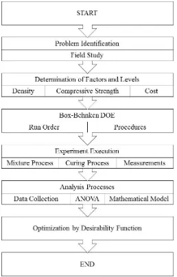
3.1 Flowchart ... 17
3.2 Problem Identification ... 18
3.3 Experiment Design Details ... 18
3.4 Experiment Execution Procedure ... 20
3.5 Data Analysis ... 22
3.6 Model Fitting ... 23
CHAPTER 4 DATA AND ANALYSIS ... 24
4.1 Experiment Results ... 24
4.2 Fitting Full Quadratic Model for Density (Y1) and Compressive Strength (Y2) ... 26
4.3 Final Selected Model ... 29
4.4 Residual Plots ... 29
4.5 Coefficient Determination Test ... 31
4.6 Test of Coefficient of Regression ... 31
4.7 Contour Plot ... 34
4.8 Surface Plots ... 37
4.9 Response Optimizer ... 38
4.10 Cost Optimization ... 40
4.11 Improvement ... 41
CHAPTER 5 CONCLUSIONS AND RECOMMENDATIONS ... 43
5.1 Conclusions ... 43
5.2 Recommendations... 43
ix
LIST OF FIGURES
Page
Fig. 1.1 Steel Pipe with Heavy Weight Concrete Coating ... 3
Fig. 1.2 Concrete weight coating processes ... 4
Fig. 2.1 Central Composite Design ...11
Fig. 2.2 Box-Behnken design...12
Fig. 3.1 Flow Chart of Research Process...17
Fig. 3.2 Standard tool and equipments...22
Fig. 4.1 Residual Plot of Y1 ...23
Fig. 4.2 Residual Plot of Y2 ...24
Fig. 4.3 Contour Plot of Y1 vs X3 and X4 at X1 = 110 and X2 = 992 With Red Line as a Constant Value of Density 3040 Kg/m3 ...28
Fig. 4.4 Contour Plot of Y1 vs X3 and X4 at X1 = 110 and X2 = 992 With Red Line as a Constant Value of Density 3040 Kg/m3 ...29
Fig. 4.5 Contour Plot of Y2 vs X3 and X4 at X1 = 110 and X2 = 992 With Red Line as a Constant Value of Compressive Strength 40 MPa...29
Fig. 4.6 Superimposed Contour Plots ...30
Fig. 4.7 Surface Plot of Y1 ...31
Fig. 4.8 Surface Plot of Y2 vs X3, X4 ...31
Fig. 4.9 Combined Response Optimizer Plot For Density and Compressive Strength at Target Values of Density 3040 kg/m3 and Compressive Strength of 40 MPa...32
xi
LIST OF TABLE
Page
Tabel 2.1 Research Map...8
Tabel 3.1 Box-Behnken Design Of Experiment For 4 Factors 1 ... 14
Table 4.1 Experiment Results ...19
Table 4.2 Model Summary of Backward Selection Steps for Y1 ...20
Table 4.3 Model Summary of Backward Selection Steps for Y2 ...22
Table 4.4 Coefficient of Determination of Final Model ...25
Table 4.5 P-Values From ANOVA Results ...26
Table 4.6 Coded Coefficients of Anova Report for Y1 ...27
Table 4.7 Coded Coefficients of Anova Report for Y2 ...27
Table 4.8 Four Data Points (Design Mixes) From The Feasible Area ...30
xiii
LIST OF EXHIBIT
Exhibit 1 Result of Experiments ... 47
Exhibit 2 Results of Real Density Measurements ... 48
Exhibit 3 Response Surfae Regression Model Y1 vs X1, X2, X3, X4 ... 49
Exhibit 4 Response Surface Regression Model Y2 vs X1, X2, X3, X4 ... 51
Exhibit 5 Response Surface Regression Model Y1 versus X1, X2, X3, X4 on Step 7... 53
Exhibit 6 Response Surface Regression Model Y2 versus X1, X2, X3, X4 on Step 6... 54
Exhibit 7 Residual Plot of Y1 on Step 7 ... 55
Exhibit 8 Residual Plot of Y2 on Step 6 ... 56
Exhibit 9 Cost Calculation ... 57
Exhibit 10 Cost of Concrete Per Ton (Current State) ... 59
1
CHAPTER 1
INTRODUCTION
1.1 Background
PT XYZ is a manufacturer of line pipe for oil and gas transportation pipeline,
and applicator of anticorrosion coating, insulation, and heavy weight concrete
(HWC) coating products. HWC is a specific design concrete with a minimum
density of 1900 kg/m3 (DNV, 2007). Normally it consist of a mixture 4 components
of coarse and fine aggregates (iron ore), portland cement and water in a certain
proportions.
Iron ores are rocks and minerals from which metallic iron can be economically
extracted. The ores are usually rich in iron oxides and vary in color from dark grey,
bright yellow, or deep purple to rusty red. The iron itself is usually found in the
form of magnetite (Fe3O4, 72.4% Fe), hematite (Fe2O3, 69.9% Fe), goethite
(FeO(OH), 62.9% Fe), limonite (FeO(OH)·n(H2O)) or siderite (FeCO3, 48.2% Fe)
(Abdou, M.I., Abuseda, H., 2014). As the cost of iron ore increases, optimizing
concrete mixture proportion for minimizing cost becomes more desirable. The
company intends to substitute the iron ore fine aggregate with other minerals which
is cheaper than the iron ore and widely availlable locally.
Indonesia is very rich of different minerals resulting from vulcanic activities.
Rock density is very sensitive to the minerals that compose a particular rock type.
Sedimentary rocks (and granite), which are rich in quartz and feldspar, tend to be
less dense than volcanic rocks. Rocks of the same type can have a range of densities.
This is partly due to different rocks of the same type containing different
proportions of minerals. Granite, for example, can have a quartz content anywhere
between 20 and 60 percent.
The densities of some minerals
Sandstone 2.2 - 2.8
Limestone 2.3 - 2.7
Andesite 2.5 - 2.8
Quartzite 2.6 - 2.8
Granite 2.6 - 2.7
Slate 2.7 - 2.8
Dolomite 2.8 - 2.9
Minerals that have density minimum of 2.6 is a candidate of substitute. The
higher the density the better. However, the availability and the price to bring the
mineral to the factory is much more important. The availability in this case is
availability of correct size, correct amount, and correct lead time so that the
production process of CWC can be performed appropriately. There are many
minerals which technically suitable for substitute, however, commercially it is not
availllable yet.
Iron sand from Lumajang which has a high content of ilmenite (Himando and
Pintowantoro, 2013) are among of the minerals that are commercially availlable for
substitute of fine aggregate (iron ore). The density of the iron sand is between 2.6
upto 3 kg/liter. The price of the material is significantly higher than crushed stone
from Rembang due to transportation distance. For that reason the crushed stone
which has density of 2.6 upto 2.9 kg/liter is choosen for the substitute of fine
aggregate of iron ore. This substitution shall maintain the CTQ characteristics of
the concrete within the acceptable limits of the industry. The main CTQ is concrete
density and compressive strength.
The proportioning of concrete materials is carried out in a continuous batching
process using belt conveyor system. The bulk materials are graded and stored in a
separate bins. Each bins have an individual variable speed belt conveyor to control
the speed of feeding and an adjustable gate to control the thickness of the material
on the belt conveyor. From individual conveyor the material is fed into a main belt
conveyor will transport all materials and feed it into the concrete mixer. The water
is fed into the mixer through a piping and flow measuring system. The concrete
3
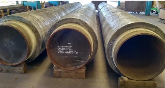
Fig. 1.1 Steel Pipe with Heavy Weight Concrete Coating
HWC coating is required to maintain subsea gas pipeline sitting on the sea-bed
thanks to its negative bouyancy. The major critical to quality (CTQ) characteristics
are density, compressive strength, water absorbtion, and impact resistant (DNV,
2007). The density is very important to get higher negative bouyancy and to
improve on bottom stability. The compressive strength and impact resistance are
important to overcome loads of installation or third party interference such as ship
anchors or trawl board impacts (DNV, 2007).
To improve its tension strength to withstand the installation loads, one layer or
more of steel reinforcement is placed within the concrete thickness. For small
diameter (OD < 14”) a galvanized wire mesh is used, while for outside diameter
more than 14 inches either reinforcement steel cage or steel wire mesh or
combination of both may be used.
HWC normally composed of coarse aggregate, fine aggregate, portland cement,
and water (Abdou, M.I., Abuseda, H., 2014). They reported that hemetite iron ore
and ilmenite ore have been successfully applied for HWC coating in Egypt. As
ilmenite contain 30% of titanium, it was to precious for HWC coating so that it was
Fig. 1.2 Concrete weight coating processes
[Source: http://www.brederoshaw.com/solutions/offshore/hevicote.html]
The compressive strength of concrete is greatly depends on the water to cement
ratio (w/c), cement, fine aggregate, and coarse aggregate proportions. Various
numbers of w/c ratio were reported 0.8 (Bauw, 2000), and 0.4 (Afi Damaris, 2011),
0.45 – 0.6 (Onwuka, Prediction of Concrete Mix Ratio Using Modified Regression
Theory, 2011). AWWA C-205 (AWWA, 2012) requires that the moisture content
shall 7% by weight of the dry mix, and the cement to fine aggregate ratio shall be
minimum 0.33 by weight. Several researchs have been performed to investigate
the relation between mix design of light weight concrete and the compressive
strength.
The type of cement shall be considered when the design life of the pipeline is
more than 20 years. The corrosion induced by chlorides from sea water may shorten
the life time of the concrete. Girardi and Di Maggio (2011) reported that concrete
shows extensive degradation when exposed to sulfate bearing solutions or polluted
ground waters. The processes leading to corrosion in concrete sewer pipes are
highly complex, still far from fully understood.
1.2 Statement of Problem
What is the optimum concrete constituents to get the best possible output in
terms of density, compressive strength, and cost? This is done by optimising the
5
combinations of constituents and then to choose the best variants of these mixtures
by comparing their density and compressive strength which will minimize the cost
by Box-Behnken approach.
1.3 Research Objectives
The objective of this research is to find out the minimum cost of the
proportion of the new design mix of HWC coating that meets the requirements.
1.4 Research Benefits
The major benefits of this research are encouraging the company of using a more precious natural resources (iron ore) efficiently, and improve competitive advantages of the company.
1.5 Definition
The scope of research is limited to the following:
1. The four components of mixture are as follow:
a. Coarse aggregate : iron ore
b. Fine aggregate : crushed stone or iron ore
c. Portland cement
d. Water
2. The CTQs of the heavy concrete to be considered are :
a. Density
b. Compression strength
c. Cost
3. The coarse aggregate is iron ore size shall be 3/8” or more.
4. The fine aggregate is either iron ore or other minerals, with size 1/6” or less.
1.6 Writing Systematic
This chapter presents the background of the research, problem indentification,
research objectives, research benefit, research scope and research outline.
• CHAPTER 2-LITERATURE REVIEW
This chapter draws on the various literatures and previous works on this
subject, theoritical background, and standards that will be used as the basis for this
research. Literatures used for this research are taken from books, journals and also
related company’s SOP.
• CHAPTER 3 - RESEARCH METHODOLOGY
This chapter explains the research stages which cover the research program,
type of data and their sources.
• CHAPTER 4- DATA ANALYSIS AND DISCUSSION
This chapter explains process of data collection which will be used for
calculation. Data is collected from the execution of the experiment. This chapter
describes how the data will be analyzed using MINITAB 17 and the result will be
interpreted.
• CHAPTER 5- CONCLUSIONS AND RECOMMENDATIONS
This chapter presents the conclsion and recommendation following the
analysis that is carried out in the previous chapter. This final chapter is expected to
fulfill the objectives of the research. Suggestion for future research will also be
7
CHAPTER 2
LITERATURE REVIEW
2.1 General Overview
Offshore gas development involves aggressive environment due to deep salt water,
severity of prevailing climatic conditions imposed by high winds, strong seas and low
temperature (Kyriakides and Edmundo Corona , 2007). Heavy aggregates of massive iron
ore is utilized in the HWC mix used for concrete coating of submarine gas pipelines which
will be immersed or laid on seabed under seawater to keep it firmly on the seabed not
moving nor floating and to protect the pipes and its supplements against mechanical
impacts.
The hostile environments and the currents on the sea floor call for coatings of sufficient weight to provide stability and of specific composition to prevent corrosion. These
characteristics are provided by two layers of coating, anticorrosion coating and concrete
coating. The concrete coatings to submarine pipelines are required to resist unique loads
and are of unusual mix proportions. This gives rise to two problems when monitoring the
quality of the coating. There is a risk of using inappropriate quality assurance techniques,
or misinterpreting their results. The main components of the concrete mix are: cement, fine
aggregates, heavy aggregates and mixing water. The cement shall be sulfate resisting
Portland cement suitable for undersea uses in preparation of the concrete. Cement shall
have a tricalcium aluminate content of not more than 3.5% and low alkali content less than
0.6% in order to attenuate the reactions of certain types of aggregates in marine
environments. The type of cement shall be considered when the design life of the pipeline
is more than 20 years.
The DNV standard (DNV, 2007) and ISO Standard (ISO:21809-5, 2010) requires that
the concrete constituents and manufacturing method shall provide the following
recommended minimum requirements to as-applied coating properties: • minimum thickness: 40 mm,
• minimum compressive strength (i.e. average of 3 core specimens per pipe): 40 MPa (ASTM C39),
• maximum water to cement ratio : 0,4 with minimum cement content shall be 400
kg/m3
To improve heavy concrete tension strength to withstand the installation loads, one
layer or more of steel reinforcement is placed within the concrete thickness. The heavy
aggregate is usually from iron ore or other type of heavy mineral. Abdou and Abuseda
reported that hemetite iron ore and ilmenite ore have been successfully applied for HWC
coating in Egypt (Abdou, M.I., Abuseda, H., 2014). As ilmenite contain 30% of titanium,
it was too precious for HWC coating so that it was replaced by hemetite iron ore.
Several works have been done by previous researchers to investigate the relation of the
design mix and the compresive strength of regular concrete. A mathematical method based
on modified regression theory is formulated for the prediction of compressive strength was
proposed by Onwuka et al (2011). Another work by Onwuka et al (2013) reported the
development of computer programmes based on simplex and modified regression theories
for designing concrete mixes to predict the compressive strength.
An optimization of mixture proportions of six components for high performance
concretes using statistical experiment design and analysis method have been developed by
Simon (2003). A further study of a mixture method and response surface method of
experimental design of high performance concrete (HPC) was performed by Simon et al
(1999). In this study Simon had three components of mixture; water, cement, and aggregate.
Simon also reported his research which is intended to investigate the feasibility of using
statistical experiment design (mixture approach) and analysis methods (factorial approach)
to optimize concrete mixture proportions and to develop an internet-based computer
program to optimize concrete mixture using these methods (Simon M. , 2003).
Optimization of mixture proportions for concrete pavements was reported by Rudy and
Olek (2012). The influence of the amount and type of supplementary cementitious materials
on selection of optimum proportions for concrete pavement mixtures was studied utilizing
Response Surface Methodology (RSM) using 3 binders system.
A response surface methodology based experimental also carried out by Lotfy et al
(2014) to model the influence of key parameters on the properties of LWSCC (Lightweight
Self-Consolidating Concrete) mixtures developed with expanded clay. Three key design
parameters were selected to derive mathematical models for evaluating fresh and hardened
9
A study of concrete aggregate optimization was reported by Lindquist (2015).
According to Lindquist to achieve an optimum gradation generally requires at least three
differently sized aggregates. The methodology was using both the modified coarseness
factor chart (MCFC) introduced by Shilstone and the percent retained chart.
Performance of concrete properties for different combined aggregate was reported by
Ashraf and Noor (2011). It is reported that the concrete conpressive strength and
workability are highly affected by its aggregate gradation. Moreover, concrete compressive
strength can be increased more than 50% just by altering its aggregate gradation.
The influence of water on the performance of concrete was investigated by Hover who
reported that the behaviour of concrete is intimately associated with water. Water is an
essential element in most of the mechanism that degrade concrete properties over time
(Hover, 2011).
The application of statistical models (response surface method) for proportioning
lightweight self-consolidating concrete was reported by Lotfy, Hossain, and Lachemi
(2014). Three key mix design parameters were selected to derive mathematical model for
evaluating fresh and hardened properties.
Muthukumar et al. (2003) studied the optimization of mix proportions of silica
aggregates for use in polymer concrete was attempted using Box-Behnken Design. High purity silica aggregates of six different standard particle sizes were chosen for the study. Void content of 54 statistically designed combinations were experimentally determined by
adopting standard technique. Using Design Expert software the results were analyzed and
an optimum composition having minimum void content was achieved. The optimum
combination had a correlation coefficient of 0.95782 which proved the fitness of the
selected model in analyzing the experimental data.
2.2 Introduction to Response Surface Methodology
The choice of an experimental design depends on the objectives of the experiment and
the number of factors to be investigated:
a. Comparative objective
If we have one or several factors under investigation, but the primary goal of your
experiment is to make a conclusion about one a-priori important factor, (in the presence of,
or not that factor is "significant", (i.e., whether or not there is a significant change in the
response for different levels of that factor), then we have a comparative problem and we
need a comparative design solution.
b. Screening objective:
The primary purpose of this experiment is to select or screen out the few important
main effects from the many less important ones. These screening designs are also termed
main effects designs.
c. Response Surface (method) objective:
The experiment is designed to allow us to estimate interaction and even quadratic
effects, and therefore give us an idea of the (local) shape of the response surface we are
investigating. For this reason, they are termed response surface method (RSM) designs.
RSM designs are used to:
• Find improved or optimal process settings. • Troubleshoot process problems and weak points.
• Make a product or process more robust against external and non-controllable influences. "Robust" means relatively insensitive to these influences.
d. Optimal fitting of a regression model objective:
If we want to model a response as a mathematical function (either known or empirical)
of a few continuous factors and we desire "good" model parameter estimates (i.e., unbiased
and minimum variance), then we need a regression design.
Response surface methods are used to examine the relationship between a response
and a set of quantitative experimental variables or factors. These methods are often
employed after a "vital few" controllable factors have been identified and it is required to
find out the factor settings that optimize the response. Designs of this type are usually
chosen when it is suspected that the response surface is curvature.
Response surface methods may be employed to:
11
• Identify new operating conditions that produce demonstrated improvement in
product quality over the quality achieved by current conditions
• Model a relationship between the quantitative factors and the response
Minitab provides two response surface designs: Central Composite Designs (CCD) and
Box-Behnken Designs (BBD).
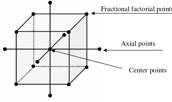
2.2.1 Central Composite Design (CCD)
The most commonly used response surface experimental design is central
composite design. Central composite designs consist of a factorial or fractional factorial
design with center points, augmented with a group of axial (or star) points that allow
estimation of curvature. we can use a central composite design to: • Efficiently estimate first- and second-order terms
• Model a response variable with curvature by adding center and axial points to a
previously-run factorial design.
A central composite design consists of a "cube" portion made up of the design points
from a factorial or fractional factorial design; 2K axial or "star" points, and center points
(where K is the number of factors). Points on the diagram below represent the experimental
runs that are performed in a 2-factor central composite design:
Fig. 2.1 Central Composite Design
Fractional factorial points
Axial points
Key features of this design include:
• Recommended for sequential experimentation since they can incorporate information from a properly planned two-level factorial experiment
• Allows for efficient estimation of quadratic terms in a regression model
• Exhibits the desirable properties of having orthogonal blocks and being rotatable or
nearly rotatable.
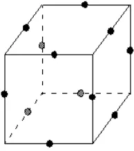
2.2.2 Box-Behnken Design (BBD)
A Box-Behnken design is a three level design in which all the design points are either: • at the center of the design
• centered on the edges of the cube, equidistant from the center
Additionally, the design points are never set at extreme (low or high) levels for all factors
simultaneously. The diagram below represents a three factor design without center points.
The points represent the experimental runs that are performed.
Fig. 2.2 Box-Behnken design
Key features of this design include:
• Allow efficient estimation of quadratic terms in a regression model
• Exhibits the desirable properties of having orthogonal blocks and being rotatable or nearly rotatable
13
• All design points fall within safe operating limits (within the nominal high and low
levels) for the process
Muthukumar, et al. (2002) had applied the RSM-BBD approach on their research for
optimization of mix proportions of silica aggregates for use in polymer concrete was attempted using statistical techniques. High purity silica aggregates of six different standard particle sizes were chosen for the study. Void content of 54 statistically designed
combinations were experimentally determined by adopting standard technique. Using
Design Expert software the results were analyzed and an optimum composition having
minimum void content was achieved. The optimum combination had a correlation coefficient of 0.95782 which proved the fitness of the selected model in analyzing the experimental data.
2.3 Heavy Weight Concrete Coating System
The objectives of a concrete weight coating are to provide negative buoyancy to the
pipeline, and to provide mechanical protection of the corrosion coating and linepipe during
installation and throughout the pipeline's operational life. The concrete weight coating
(thickness, strength, density, amount of reinforcement) shall be designed for the specific
project; i.e. the actual installation, laying and operation conditions for the pipeline shall
then be taken into consideration. For materials and application of concrete weight coating
requirements in ISO 21809-5 shall apply with the additional and modified requirements.
The following modification of acceptance criteria for inspections and tests during PQT
shall apply:
• The thickness of the concrete coating shall not be less than 40 mm
• The minimum in-situ compressive strength of the concrete coating shall not be less than 40 MPa. The mean strength shall be calculated from compressive test results
of three drilled cores obtained from one pipe, with no single test results less than 34
MPa.
• The minimum density shall be 3040 kg/m3.
• The concrete coating shall be reinforced by steel bars welded to cages or by wire mesh steel. The minimum percentage of the steel reinforcement shall be 0.5%
concrete coating. The minimum diameter of circumferential cage reinforcement
shall be 5 mm. The maximum spacing between circumferential and longitudinal
cage reinforcement shall be 125 mm and 250 mm, respectively. The minimum
diameter of wire mesh reinforcement shall be 2 mm. The minimum overlap of wire
mesh reinforcement shall be 1.5 x distance between the wires or 25 mm (whichever
is greater). Minimum concrete cover to the reinforcement shall be 15 mm for
concrete thickness less or equal to 50 mm and minimum 20 mm for concrete
thickness greater than 50 mm. The thickness of the concrete coating shall not be
less than 40 mm.
All those standard requirements shall be maintained and fulfilled with the new concrete
mixture design. Minerals that have density minimum of 2.2 is a candidate of substitute. The
higher the density the better. However, the availability and the price to bring the mineral to
the factory is much more important. The availability in this case is availability of correct
size, correct, amount, and correct lead time so that the production process of CWC can be
performed as per schedule.
2.4 Research Mapping
Several works have been done previosly with various materials, CTQ, and methods.
Muthukumar et al (2003) have used Box-Behnken design of experiment to optimize 6 silica
sizes for obtaining mixture with minimum voids. It was concluded that out of the six different particle sizes chosen for the study, only three of them were found to be sufficient for obtaining a mix with minimum void content. A full mapping of several previous
researchs is presented in Table 2.1.
Tabel 2.2 Research Map
Author / Year Title Descriptions Catagories Results
15
Author / Year Title Descriptions Catagories Results
17
CHAPTER 3
RESEARCH METHODOLOGY
This research is a design of experimental. The major factors that have a significant
influences to the response have been identified by previous research and international
standards and the main objective is yo minimize cost. For that reason Response Surface
Methodology is choosen, and Box-Behken design is selected because this design require
less sample with a good result.
3.1 Flowchart
3.2 Problem Identification
Based on field and literature studies the CTQ of heavy concrete is affected by four factors :
1. Water
2. Portland Cement 3. Fine Aggregate 4. Coarse aggregate
For the purpose of this study all materials will be chosen from the one available at PT XYZ as follow:
• Water : potable water
• Portland Cement : The cement is type 2 produced by PT SEMEN TIGA RODA, CIBINONG. It shall comply with the requirements of ASTM C150.
• Fine Aggregate : The crushed stone is from Rembang 1 mining area, with size 1/6” or less
• Coarse aggregate : The iron ore for heavy aggregate is from Pelaihari mining site, South Kalimantan. It shall conform to ASTM C33. The coarse aggregate is iron ore size shall be 3/8” or more.
3.3 Experiment Design Details
Selecting an appropriate experiment design depends on several criteria, such as ability to estimate the underlying model, ability to provide an estimate of repeatability, and ability to check the adequacy of the fitted model. The “best” experiment design depends on the choice of an underlying model which will adequately explain the data. For this experiment, the following quadratic Scheffé polynomial was chosen as a reasonable model for each property as a function of the four components:
y = b1X1+…+ b4X4 + b12X1X2 +…+ b34X3X4 +b11X12+ b22X22 + b33X32+ b44X42+ e (3.1)
where :
X1 = water proportion, X2 = cement proportion, X3 = fine aggregate proportion, X4 = coarse
aggregate proportion.
In the analysis of Response Surface Design, Minitab fits a typical model with main
effects, two-factor interactions, and quadratic effects. If any of higher-order terms are not
significant in the first analysis, they can be removed from the model until all remaining
19
the Minitab Response Optimizer, factor setting to maximize, minimize, or find a target
value are easy to identify.
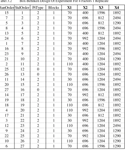
Based on the requirement of DNV-OSF-101 (DNV, 2007) and ISO 21809-5 (ISO:21809-5, 2010) it is determined that the levels of 4 (four) factors as follow in kilograms:
Factor 1 = X1 = water minimum 30 and maximum 110
Factor 2 = X2 = cement minimum 400, and maximum 992
Factor 3 = X3 = fine aggregate, minimum 812, and maximum 1596
Factor 4 = X4 = heavy aggregate, minimum 1290, and maximum 2494
Tabel 3.2 Box-Behnken Design Of Experiment For 4 Factors 1 Replicate
Source : Minitab 17
3.4 Experiment Execution Procedure
Before conducting the experiment, review the following guidelines and complete the
appropriate activities:
1. Train individuals involved in the experiment : Because errors in the experimental
procedures can invalidate the results of an experiment, all procedures should be carefully
RunOrder StdOrder PtType
Blocks
X1
X2
X3
X4
21
documented and individuals trained on those procedures (Montgomery & Runger,
2011). Include the following:
• Specify how to measure the response and note any special techniques that may be required.
• Stipulate how to set factor levels. Make sure everyone understands how to set the factors at each level.
• Explain how to set up the equipment for runs. For example, each time the
machine settings is changed, the machine shall be run at the new settings until
it stabilizes before collecting the measurements for the experiment.
• Develop plans for troubleshooting. Communicate how to handle potential problems, such as missing measurements.
• Specify how to record special circumstances. Explain how to track any
changes in conditions that may occur while the data is being collected.
2. Validate measurement system : to trust the experimental results, it is needed to verify
that the measurement system is accurate. The measurement systems that are used both
to measure the response and to set the factor levels should be verified.
3. If the experiments are part of a larger improvement project, such as a six sigma project,
the measurement system for the response should have been validated previously. Make
sure that the measurement system had been verified for the factors as well.
4. Check all design combinations. After the design is created, the actual combinations of
factor settings for each experimental run need to be reviewed to make sure they are
feasible and safe to run.
5. Perform trial runs. Performing trial runs before running an experiment is useful, if time
and budget permits. Trial runs will allow to:
• Assess the consistency of materials in the experiment. • Check the measurement systems for the experiment.
• Test the experimental procedures and ensure that operators perform them correctly.
Based on the Box-Behnken design table, the experiment shall be executed
sequentially in accordance with the run-order (Montgomery & Runger, 2011). The
proportion limits of each factors shall be measured and controlled using appropriate tools
and equipments.
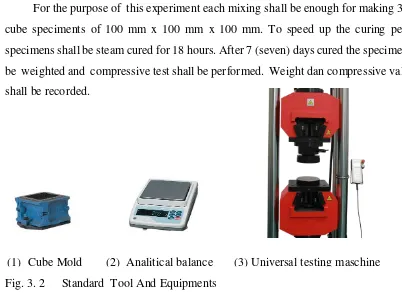
For the purpose of this experiment each mixing shall be enough for making 3 (three)
cube speciments of 100 mm x 100 mm x 100 mm. To speed up the curing period all
specimens shall be steam cured for 18 hours. After 7 (seven) days cured the specimens shall
be weighted and compressive test shall be performed. Weight dan compressive value data
shall be recorded.
Fig. 3. 2 Standard Tool And Equipments
3.5 Data Analysis
The relationship between data (density and compressive values) as a response to the
4 (four) quantitative experimental variables (factors) will be analized using Response
surface methods. The density response (Y1), the compressive strength response (Y2) and
the combined response (Y3 = Y1 + Y2) will be analyzed and optimized. A matemathical
regression model will be generated for each responses and its combination as a function of
each factors. We want to find the factor settings that optimize the response. Each response
will be plotted against X3 (crushed stone) and X4 (iron ore) while assume the other factors
are constant. A minimum acceptable value for compressive strength is 40 MPa, and density
3040 kg/m3. The feasible factor space for the mixture experiment of four components can
be determined. Cost analysis will be carried out to find out the minimum cost of the new
mixture.
23
Using Analyze Response Surface Design from MINITAB 17 to fit a model to data
collected using Box-Behnken, and choose to fit models with the following terms: linear
terms, squared terms, interaction terms.
From the analysis of variance table we will use the p-values to determine which of
the effects in the model are statistically significant. Typically we look at the interaction
effects in the model first because a significant interaction will influence how we interpret
the main effects.
3.6 Model Fitting
S, R2, adjusted R, and predicted R obtained from the MINITAB data analysis are
measures of how well the model fits the data. The fit is the predicted mean of the response
at these variable settings.
From the regresion equation the fitted value can be calculated and the smaller the
difference between the oberved value from the fitted value the better the model.
3.7 Optimization
Using Minitab's Response Optimizer we will identify the variable settings that
optimize a single response or a set of responses. For multiple responses, the requirements
CHAPTER 4
DATA AND ANALYSIS
Based on the data collected from the execution of the experiment, a matemathical
model will be developed for the correlation between factors (water, cement, crushed stone,
and iron ore) and responses (density, compressive strength). An optimization will then be
performed based on the following criteria:
1. Minimum density = 3040 kg/m3
2. Compressive strength = 40 MPa
Both criterion are the the factors which fulfill the above mentioned criteria and have the
lowest price will be choosen as an optimum solution.
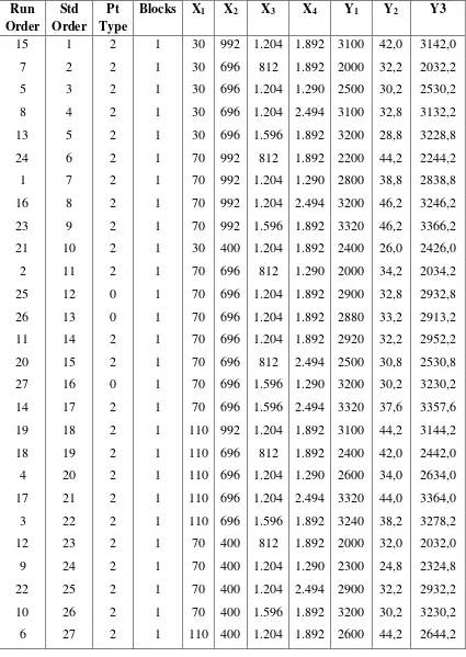
4.1 Experiment Results
The experiment have been executed resulting 27 cube samples of the individual mix
from 27 runs in accordance with the Box-Behnken design table. After the samples cured,
the samples are weighed and the individual weight are recorded. For example, the weight
of sample #1 = 3100 grams = 3,100 kilograms. The volume of the cubes is 0,1 x 0,1 x 0,1
m3 = 0,001 m3. The density of sample #1 = 3100 kg/m3. After all the density of the samples
are known, the sample is put on the universal testing machine in the same sequence as
before. The compression test is done, and the compressive strength is recorded. For
example sample number 1 has compressive strength of 42,0 MPa. A complete results of the
test is presented on Table 4.1 where the responses are densities (Y1) in Kilograms per cubic
meter (kgs/m3) and compressive strength (Y2) in Mega Pascal (MPa). The combined
response Y3 = Y1 + Y2 without unit is presented for optimization analysis purpose.
The table is then analyzed using statistics software MINITAB 17. Response Surface
Regression with Backward Elimination of Terms is chosen. The result is presented and
discussed in the following sections. A complete statistical results are presented on the
25 Table 4.1 Experiment Results
4.2 Fitting Full Quadratic Model for Density (Y1) and Compressive Strength (Y2)
The relation of density and compressive strength with its constituents (water, cement,
crushed stone, and coarse aggregate) is analyzed with Minitab 17. The influences of each
factors (terms) to the responses (Y1 and Y2) is analyzed using regression model and
ANOVA. In the analysis of Response Surface Design, Minitab fits a typical model with
main effects, two-factor interactions, and quadratic effects. Minitab provide options of
methods for RSM analysis: forward selection, backward selection, forward and backward
selection, and best subset regression. In this case Regression Model is carried out using
Backward Selection whereby all terms are included in the initial run, and terms with the
highest P-value which is not significant will be removed. The process of removing the worst
remaining terms continues until the model stops getting better.
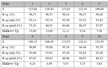
The backward selection process of Y1 versus X1, X2, X3, X4 (see Exhibit 1)
required 10 steps to get all low P-values, while for Y2 required 7 steps, and for Y3 required
9 steps (Exhibit 11). It is very important to assess the model as a whole. Tabel 4.2 listing
the statistical report of each steps. The detail report of the Response Surface Regression for
Y1 see Exhibit 3.
Table 4.2 Model Summary of Backward Selection Steps of Y1
Steps 1 2 3 4 5
In Step 2 (Table 4.2), the term with the highest p-value 0,951 (term X4*X4) was
removed, and the model getting better indicated by reducing the standard deviation S from
27
The coefficient of determination for the model R-sq or R2 is high (96,37%), which
mean that 96,37% of variation explained by the model. The higher R-sq the better. On the
step 2 the R-sq value not change, but the value of R-sq (adj) and R-sq (pred) is increasing
from 92,14 to 82,74 for R-sq (adj) and 79,16 to 80,91 respectively so that removing X4*X4
made the model better.
R-sq (adj) includes an adjustment to R-sq which reduces the adjusted R-sq for every
term removed from the model. This is a safeguard against over-fitting. A model with too
many variables may have high R-sq, but no good at prediction. In general, the best model
has the highest value of adjusted R-sq.
Mallows’ Cp is an attempt to balance the risks of too many variables with the risks of too few variables (Sleeper, 2012). Mallows' Cp is a measure of goodness-of-prediction.
The formula is: (SSEp / MSEm) - (n - 2p) where SSEp is SSE for the model under
consideration, MSEm is the mean square error for the model with all predictors included,
n is the number of observations, and p is the number of terms in the model, including the
constant. In general, look for models where Mallows' Cp is small and close to p. A small
Cp value indicates that the model is relatively precise (has small variance) in estimating the
true regression coefficients and predicting future responses. Models poor predictive ability
and bias have values of Cp larger than p (Minitab, 2010). According to Montgomerry
(Montgomery & Runger, 2011) The regression equation that have neglicable bias will have
values of Cp that close to p, while those with significant bias will have values of Cp that
are significantly greater than p. This initial model has 15 terms so that p = 15.
The highest P-value in Step 2 is 0,742 belong to term X2*X3. This term is removed
in Step 3. The S value is getting smaller, the R-sq (Adj) and R-sq (pred) are getting larger
so that removing X2*X3 make the model better. Slight reduction of the coefficient of
determination R-sq is still acceptable. This improvement continues in Step 4 by removing
X1*X4, Step 5 (removing X1*X1), Step 6 (removing X2*X4), and Step 7 (removing
X1*X2). However, on Step 8 (removing X1*X3) the model getting worse: S increase,
R-sq, R-sq (adj) and R-sq (pred) are decreasing.
Starting from Step 8 upto Step 10 the model is getting worse and and worse. S
increasing from the lowest 108,65 (Step 7) to 113,53 (Step 8), 118,21 (Step 9) and 122,69
(Step 10). R-sq decreasing from 95,8 (Step 7) to 95,16, 94,48, 93,76. R-sq (adj) decresing
from 93,93 (Step 7) to 93,38, 92,82, 92,28. Having this situation it is concluded that
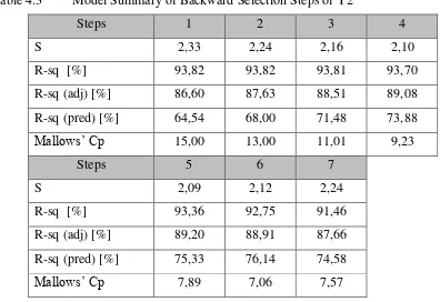
Table 4.3 Model Summary of Backward Selection Steps of Y2
Steps 1 2 3 4
S 2,33 2,24 2,16 2,10
R-sq [%] 93,82 93,82 93,81 93,70
R-sq (adj) [%] 86,60 87,63 88,51 89,08
R-sq (pred) [%] 64,54 68,00 71,48 73,88
Mallows’ Cp 15,00 13,00 11,01 9,23
Steps 5 6 7
S 2,09 2,12 2,24
R-sq [%] 93,36 92,75 91,46
R-sq (adj) [%] 89,20 88,91 87,66
R-sq (pred) [%] 75,33 76,14 74,58
Mallows’ Cp 7,89 7,06 7,57
Similarly for response Y2 (compressive strength) on Table 4.3. Step 2 to Step 6
greatly improve the selected model:
• S reduced from : 2.33 to 2,12
• R-sq : 93,82 to 92,75
• R-sq (Adj) : 86,60 to 88,91 • R-sq (pred) : 64,54 to 75,14
However, Step 7 (removing X1*X4) tends to make the Y2 model worst, i.e. S increase to
2,24157, R-sq decrease to 91,46, R-sq (Adj) to 87,66, and R-sq (pred) to 74,58. For that
reason the backward selection of Y2 model is stopped at Step 6.
Similarly for response Y3 = Y1 + Y2 (see Exhibit 11), after step 7 the model is
getting worse. For that reason the backward selection of Y3 model is ended at step 7. For
29 4.3 Final Selected Model
The final model to be selected and the ANOVA is presented at Exhibit 5 and Exhibit
6 for Density (Y1) and Compressive Strength (Y2) respectively. These model shall be
assessed and evaluated with several relevant tests.
The Response Surface Regression Equation in Uncoded Units for model of Y1 is
as follow:
Y1 = -3255 + 8,91 X1 + 1,822 X2 + 4,730 X3 + 0,892 X4 - 0,000839 X2*X2
- 0,000918 X3*X3 - 0,00574 X1*X3 - 0,000403 X3*X4 ... (4.1)
The Regression Equation in Uncoded Units for Y2 is as follow:
Y2 = 51,6 + 0,004 X1 ˗ 0,0168 X2 - 0,02254 X3 - 0,01481 X4 + 0,001422 X1*X1 +
0,000044 X2*X2- 0,000338 X1*X2 + 0,000077 X1*X4 + 0,000011 X3*X4
... (4.2)
4.4 Residual Plots
To assess and diagnose common regression problems it is a convenient way to have
a graphical presentation. Figure 4.1 and Figure 4.2 provide a four-in-one residual plots of
density response (Y1) and compressive strength response (Y2).
The normality test of the residual is on the top-left of Fig. 4.1. All data points is distributed
around linear red line and it is proven to be normal. Because the number of data is more
than 15 data points, normality is not an issue.
The distribution of residual against Observation Order shows a random distribution and no
trend, shift, or cyclical pattern. There is one observation which has a large residual. It is
observation no. 26 (red arrow) with residual 195,7. This large residual may be rooted from
several sources, e.g. in accuracy of sample preparation because sequentially it is almost at
the end of the experiment, variation of aggregate size distribution, etc. Due to time
constraints that it is not possible to redo the experiment this data point is not replaced.
Large residual can be identified from Residuals vs Fits Plot. It is observation no. 26. No
clusters, unusual X-values, or unequal variation observed.
Fig. 4.2 Residual Plot of Y2
The case for compressive strength (Y2) is about the same as for density (Y1). The
distribution of residual against Observation Order shows a random distribution and no
trend, shift, or cyclical pattern. One data point has a large residual and is not well fit by the
equation. This point is marked by red arrow on the top right and bottom right and is in row
31
measurement error, curing process error, etc. Due to time constraints that it is not possible
to redo the experiment this data point is maintained.
The normality test of the residual is on the top-left of Fig. 4.2. and all data points is
distributed along the linear line it is considered to be normal. Because the number of data
is more than 15 data points, normality is not an issue.
4.5 Coefficient Determination Test
From Exhibit 5 and Exhibit 6, both models can be summrized as follow:
Table 4.4 Coefficient of Determination of Final Model
S R-sq R-sq (Adj) R-sq (pred)
Y1 108,65 95,80% 93,93% 89,63%
Y2 2,12 92,75% 88,91% 76,14%
The value of coefficient determinations R-sq for both density and compresive strength are
above 90%, which mean that the percentage of variation explained by the models is 96,8%
and 92,75% respectively so that both model pass the coefficient of determination test
requirement.
4.6 Test of Coefficient of Regression
This test is carried out based on the following hypotheses at = 0,05:
H0: Every βi does not affect the response (1 2 ...k 0)
Table 4.5 P-value From ANOVA Results
Model Density (Y1) Compressive Strength (Y2)
Regression 0,000 0,000
Linear 0,000 0,000
Quadratic 0,010 0,001
Interaction 0,081 0,002
This test to evaluate the influence of each factors in the model. The interaction
between factors shall be evaluated first because interaction may influence other factors
(Kuehl, 2000). Table 4.5 shows that the P-value of interaction for Y1 is greater than 0,05
so that H0 fail to be rejected, it may be interpreted that interaction between factors may
have influence to the density response but the influence not significant statistically.
Although the interaction statistically has no significant affect but it is decided to maintain
in the model because eliminating it will make the model getting worst as explained in
Section 4.2.
Meanwhile P-value of interaction for Y2 is less than 0,05, so that H0 shall be
rejected. Meaning that interaction between water, cement, crushed stone, and iron ore
coarse aggregate have statistically significant influence to compressive strength of the
concrete.
The P-values of Regression, Linear, and Quadratic models are less than 0,05 so that
the null hypotheses shall be rejected and conclusion can be drawn that those models have
33
Table 4.6 Coded Coefficient of ANOVA Report for Y1
Coded Coefficients
From the above table there are 3 terms which have P-value greater than 0,05, i.e. X2*X2,
X1*X3, and X3*X4 but removing it from the model only make it getting worse so that it
is considered to maintained in the model.
Table 4.7 Coded Coefficient of ANOVA Report for Y2
Coded Coefficients
X1*X4. The same condition with before those terms are maintained in the model because
4.7 Contour Plot
For the contour plot of Y1 against X3, X4 is made by setting X1 and X2 constant.
In this case X1 = 110 and X2 = 992. The contour plot of Y1 is presented on Fig. 4.1
Fig. 4.3 Contour Plot of Y1 vs X3 and X4 at X1 = 110 and X2 = 992 With Red Line as
a Constant Value of Density 3040 Kg/m3
In the contour plot, a constant density line can be drawn against X3 and X4. The
feasible space solution for density equal or greater than 3040 kg/m3 is from the red line to
the upper right area of the contour plot. This area is also presented in Figure 4.2.
In Figure 4.3 a contour plot of compressive strength against X3 and X4 with X1 =
110 and X2 = 992 is presented. A feasible space solution for minimum compresive strength
of 40 MPa is from redline to the upper right area of the plot.
Combining Fig. 4.1 and Fig. 4.3 will give visual graphical idea how a feasible space
solution which fulfill both requirements of minimum density 3040 kgs/m3 and minimum
compressive strength of 40 MPa. The feasible space salution in this case is a possible
design mix which statistically may produce concrete whose density > 3040 kg/m3 and
35
Fig. 4.4 Contour Plot of Y1 vs X3 and X4 at X1 = 110 and X2 = 992 With Red Line as
a Constant Value of Density 3040 Kg/m3
Fig. 4.5 Contour Plot of Y2 vs X3 and X4 at X1 = 110 and X2 = 992 With Red Line as
Superimposing Fig. 4.3 over Fig. 4.1, we can find a joint feasible space solution
for Y1 and Y2 graphically (Fig. 4.4). From this picture four (4) data points (design mixes)
will be taken for optimization.
Fig. 4.6 Superimposed Contour Plots
Table 4.8 Four Data Points (Design Mixes) From the Feasible Area
Points X1 X2 X3 X4 Y1 Y2
A 110 992 1593,56 1340,35 3166 40
B 110 992 1500,47 1323,68 3103 40
C 110 992 1430,64 1307,01 3042 40
4.9 Response Optimizer for Y1 and Y2
Use response optimization to help identify the combination of input variable
settings that jointly optimize Y1 and Y2 responses. Joint optimization must satisfy the
requirements for Y1 and Y2 responses in the set, i.e. minimum 3040 kg/m3 and minimum
40 MPa respectively, which is measured by the composite desirability. Desirability assess
how well a combination of input variables satisfies the goals you have defined for the
responses. Individual desirability (d) evaluates how the settings optimize a single response;
composite desirability (D) evaluates how the settings optimize a set of responses overall.
Desirability has a range of zero to one. One represents the ideal case; zero indicates that
one or more responses are outside their acceptable limits.
Fig. 4.9 Combined Response Optimizer Plot For Density and Compressive Strength
at Target Values of Density 3040 kg/m3 and Compressive Strength of 40 MPa.
According to Fig. 4.9 the join optimum factors (design mix) which the responses
fulfill the minimum requirements of density 3040 Kg/m3 and compressive strength 40 MPa
and with composite desirability 0,9982 are as follow:
39 Table 4.9 Response Optimization: Y1 and Y2
Parameters
Response Goal Lower Target Upper Weight Importance
Y2 Target 32 40 48 1 1
Y1 Target 2600 3040 3400 1 1
Solution
Y2 Y1 Composite Solution X1 X2 X3 X4 Fit Fit Desirability 1 93,9251 400 1239,64 2494 39,9826 3039,35 0,998178
Multiple Response Prediction
Variable Setting X1 93,9251 X2 400 X3 1239,64 X4 2494
Response Fit SE Fit 95% CI 95% PI Y2 39,98 2,08 (35,45; 44,51) (33,17; 46,80) Y1 3039 110 ( 2800; 3279) ( 2679; 3400)
According to the response optimizer of Y3 = Y1 + Y2 in Fig. 4.10, the optimum solution is as follow:
X1 = 71,1; X2 = 717,1; X3 = 1270,6; X4 = 2034,9
Fig. 4.10 Response Optimizer Plot For Y3 = Y1 + Y2 at Target Values of Density
(Y1) 3040 kg/m3 and Compressive Strength of 40 MPa (Y2)
4.10 Cost Optimization
Cost optimization is based on the design mixes collected from two methods of
optimization: joint optimization plot of Y1 and Y2 and optimization plot of Y3.
The cost calcultions are based on the unit price of materials are as follow:
PX1 = 0,6 USD/Ton; PX2 = 104 USD/Ton; PX3a = 20 USD/Ton; and PX4 = 80 USD/Ton.
Method 1 :
X1 = 93,92 X2 = 400 X3a = 1239,64 X4 = 2494,0
Total cost = 93,92 x 0,6 + 400 x 104 + 1239,64 x 20 + 2494,0 x 80 = 265.969,16 USD
Total weight of mix = X1 + X2 + X3 + X3a + X4 = 4227,6 tons
Cost per unit weight of heavy weight concrete = 265.969,16/4227,6 USD/Tons = 62,91
41 Method 2 :
X1 = 71,1; X2 = 717,1; X3 = 1270,6; X4 = 2034,9
Total cost = 71,1 x 0,6 + 717,1 x 10⁴ + 1270,6 x 20 + 2034,9 x 80 = 262.825,06 USD
Total weight of mix = X1 + X2 + X3 + X3a + X4 = 4093,7 tons
Cost per unit weight of heavy weight concrete = 262.825,06 /4093,7 USD/Tons = 64,20
USD/Ton
The unit cost of materials are collected at the time of writing from the purchasing
department of PT XYZ. The consumption of materials is collected from production
engineering of PT XYZ. Cost calculation example and cost calculation table is presented
in Exhibit 8. Among of two methods it is proven that data point # 1 gives the lowest total
cost of material. This design mix consist of :
• Water = 93,92 liters
• Cement = 400 kgs
• Crushed stone = 1239,64 kgs • Coarse aggregate = 2494,0 kgs
The total cost of the material following the most optimum design is 62,91 USD/Ton.
4.11 Improvement
Evaluating the current states of concrete coating production practice, there is
potential improvement can be made out of this research. The unit cost of material for one
ton concrete production using the existing material with fine aggregate of iron ore is 77,7
USD (see Exhibit 10). A potential improvement from the use of crushed stone to substitute
fine iron ore are: (77,7 – 62,91) x 100% / 77,7 = 19 %
It should be noted that this experiment have been designed with some assumptions
and exclutions. Validation shall be required to investigate the correctness between the
Based on the problem statement “What is the optimum concrete constituents to get the best possible output in terms of density, compressive strength, and cost?”, the answer is method
1.
Concrete mixture involve a chemical reaction which the result is depend not only the
constituents but also the reaction temperature which is not considered in this research. The
percentage of aggregate sizes (sieve analysis) may also have influences to the properties of
43
CHAPTER 5
CONCLUSIONS AND RECOMMENDATIONS
5.1 Conclusions
1. The optimum design mix that produce concrete with minimum density of 3040 kg/m3
and compressive strength of 40 MPa with the lowest cost of materials shall consist of : • water (93,9 liters) or 0,07 by volume
• cement (400 kgs) or 0,10 by volume
• crushed stone (1239,6 kgs) or 0,36 by volume • coarse aggregate (2494 kgs) or 0,47 by volume
2. The total cost of the material following the most optimum design is 62,91 USD/Ton.
3. There is a potential improvement or saving of 19 % from the current state based on
the optimized design mix from this research.
4. The mathematical model of the density response and compressive strength response
are as follow:
Density = -3255 + 8,91 Water + 1,822 Cement + 4,730 CrushedStone + 0,892 IronOre
- 0,000839 Cement2- 0,000918 CrushedStone2- 0,00574 Water*CrushedStone
- 0,000403 CrushedStone*IronOre
Compressive Strength = 51,6 + 0,004Water ˗ 0,0168Cement - 0,02254 CrushedStone -
0,01481 IronOre + 0,001422 Water2 + 0,000044 Cement2- 0,000338 Water*Cement +
0,000077 Water*IronOre + 0,000011 CrushedStone*IronOre
5.2 Recommendations
1. The effect of aggregate gradations and mixture temperature is not included in this
research. A more detail research including those factors is recommended.
2. The effect of factors under consideration to the impact and shear properties of concrete
are not studied. This poperties is important for the integrity of concrete coated linepipe
REFERENCES
Abdou, M.I., Abuseda, H. (2014), “New Heavy Aggregate for Offshore Petroleum Pipeline Concrete Coating Central West Sinai, Egypt”, Egyption Journal of Petroleum, Vol. 105, P. 301 – 312.
Achmad, S., Alghamdi, S.A., (2014), “A Statistical Approach to Optimizing Concrete Mixture design”, The Scientific World Journal, Vol. 2014, Article ID 561539, 7 pages
ACI Committee 211 (1991), Standard Practice for Selecting Proportions for Normal, Heavyweight, and Mass Concrete, The American Concrete Institute, Detroit.
ACI Committee 304 (1996), Heavyweight Concrete: Measuring, Mixing, Transporting, and Placing, The American Concrete Institute, Detroit.
Afi Damaris, R. (2011), Optimasi Kuat Tekan Dan Daya Serap Air Dari Batako Yang Menggunakan Bottom Ash Dengan Pendekatan Respon Serentak, Tesis, MMT-ITS, Surabaya
ANSI/AWWA C205, (2012), Cement Mortar Protective Lining and Coating for Steel Water Pipe – 4 In. (100 mm) and Larger – Shop Applied, American Water Work Association, Denver.
Barbuta, M., Lepadatu, D. (2008), “Mechanical Characteristic Investigation of Polymer Concrete Using Mixture Design of Experiments and Response Surface Method”,
Journal of Applied Sciences, Vol. 8 No. 12, pp. 2242-2249.
Bauw, Lila, (2000), Analisis komposisi optimal proses pembuatan batako dengan pendekatan taguchi robust design, Tesis, MMT-ITS, Surabaya.
DNV OS-F101, (2007), Offshore Standard DNV-OS-F101 Submarine Pipeline Systems, Det Norsk Veritas, Norway.
Esmaeili, A. (2012), “Simulation of a Sub-Sea Gas Pipeline in Persian Gulf to Estimate the Physical Parameters”, Procedia Engineering, Vol. 42, p. 1634 – 1650.
Girardi, F., Di Maggio, R. (2011), “Resistance of Concrete Mixtures to Cyclic Sulfuric Acid Exposure and Mixed Sulfates: Effect of the Type of Aggregate”, Cement & Concrete Composites, Vol. 33, p. 276 – 285.
45
Haddad, H., Al Kobaisi, M. (2013), “Influence of Moisture Content on the Thermal and Mechanical Properties and Curing Behavior of Polymeric Matrix and Polymer Concrete Composite”, Materials and Design, Vol. 49, p. 850 – 856.
Kuehl, Robert O., (2000), Design of Experiments : Statistical Principles of Research Design and Analysis, 2nd edition, Duxbury Thomson Learning, Pacific Grove.
Luftig, Jeffrey T. and Jordan, Victoria S., (1998), Design of Experiments in Quality Engineering, McGraw-Hill, New York.
Lindquist, W., Darwin, D., Browning, J., McLeod, H.A.K., Yuan, J., Reynolds, D., “Implementation of Concrete Aggregate Optimation”, Construction and Building Materials, Vol. 74, 2015, pp. 49-56
Minitab Inc. (2010). "DOE," Getting Started with Minitab 17, downloaded from www.minitab.com.
Montgomery, Douglas C. and Runger, George C. (2009), Applied Statistics and Probability for Engineers, 5th edition, SI Version, John Wiley & Sons, Inc. Asia.
Muthukumar, Mohan, Rajendran (2003), “Optimization of mix proportions of mineral aggregates using Box-Behnken design of experiments”, Cement & Concrete Composites, 25 (2003) 751–758
Myers, Raymond H. and Montgomery, Douglas C., (2002), Response Surface Methodology : Process and Product Optimization Using Designed Experiments, 2nd edition, John Wiley & Sons, Inc., New York.
Onwuka, D.O., Okere, C.E., Arimanwa, J.I, Onwuka, S.U. (2011), “Prediction of Concrete Mix Ratio Using Modified Regression Theory”, Computerized Method of Civil Engineering, Vol. 2 No. 1, pp. 95-107
Onwuka, D.O., Okere, C.E., Arimanwa, J.I, Onwuka, S.U. (2013), “Computer Aided Design of Concrete Mixes”, International Journal of Computational Engineering Research, Vol. 3 No. 2, pp. 67-81
Rudy, A., Olek J., (2012), Optimization of Mixture Proportions for Concrete Pavements— Influence of Supplementary Cementitious Materials, Paste Content and Aggregate Gradation, Joint Transportation Research Program, Indiana Department of Transportation and Purdue University, Purdue University, West Lafayette, Indiana.
![Fig. 1.2 Concrete weight coating processes [Source: http://www.brederoshaw.com/solutions/offshore/hevicote.html]](https://thumb-ap.123doks.com/thumbv2/123dok/1748943.2089664/20.595.169.423.119.240/concrete-coating-processes-source-brederoshaw-solutions-offshore-hevicote.webp)