Think Complexity Ebook free download

(1)

Think Complexity

(2)

(3)

Think Complexity

Version 1.1

Allen B. Downey

(4)

Printing history:

Fall 2008: First edition.

Fall 2011: Second edition.

Green Tea Press 9 Washburn Ave Needham MA 02492

Permission is granted to copy, distribute, transmit and adapt this work under a Creative Com-mons Attribution-NonCommercial-ShareAlike 3.0 Unported License: ❤tt♣✿✴✴❝r❡❛t✐✈❡❝♦♠♠♦♥s✳

♦r❣✴❧✐❝❡♥s❡s✴❜②✲♥❝✲s❛✴✸✳✵✴.

If you are interested in distributing a commercial version of this work, please contact Allen B. Downey.

The original form of this book is LA_{TEX source code. Compiling this L}A_{TEX source has the effect of} generating a device-independent representation of the book, which can be converted to other formats and printed.

The LA_{TEX source for this book is available from} ❤tt♣✿✴✴❣r❡❡♥t❡❛♣r❡ss✳❝♦♠✴❝♦♠♣❧❡①✐t② ❤tt♣✿✴✴❝♦❞❡✳❣♦♦❣❧❡✳❝♦♠✴♣✴❝♦♠♣❧❡①✐t②

This book was typeset using LA_{TEX. The illustrations were drawn in xfig.}

The cover photo is courtesy of❜❧♠✉r❝❤, and is available under a free license from❤tt♣✿✴✴✇✇✇✳

(5)

Preface

0.1

Why I wrote this book

This book is inspired by boredom and fascination: boredom with the usual presentation of data structures and algorithms, and fascination with complex systems. The problem with data structures is that they are often taught without a motivating context; the problem with complexity science is that it is usually not taught at all.

In 2005 I developed a new class at Olin College where students read about topics in com-plexity, implement experiments in Python, and learn about algorithms and data structures. I wrote the first draft of this book when I taught the class again in 2008.

For the third offering, in 2011, I prepared the book for publication and invited the students to submit their work, in the form of case studies, for inclusion in the book. I recruited 9 professors at Olin to serve as a program committee and choose the reports that were ready for publication. The case studies that met the standard are included in this book. For the next edition, we invite additional submissions from readers (see Appendix A).

0.2

Suggestions for teachers

This book is intended as a scaffold for an intermediate-level college class in Python pro-gramming and algorithms. My class uses the following structure:

Reading Complexity science is a collection of diverse topics. There are many intercon-nections, but it takes time to see them. To help students see the big picture, I give them readings from popular presentations of work in the field. My reading list, and suggestions on how to use it, are in Appendix B.

Exercises This book presents a series of exercises; many of them ask students to reimple-ment seminal experireimple-ments and extend them. One of the attractions of complexity is that the research frontier is accessible with moderate programming skills and under-graduate mathematics.

(6)

Case studies In my class, we spend almost half the semester on case studies. Students participate in an idea generation process, form teams, and work for 6-7 weeks on a series of experiments, then present them in the form of a publishable 4-6 page report. An outline of the course and my notes are available at❤tt♣s✿✴✴s✐t❡s✳❣♦♦❣❧❡✳❝♦♠✴s✐t❡✴

❝♦♠♣♠♦❞♦❧✐♥.

0.3

Suggestions for autodidacts

In 2009-10 I was a Visiting Scientist at Google, working in their Cambridge office. One of the things that impressed me about the software engineers I worked with was their broad intellectual curiosity and drive to expand their knowledge and skills.

I hope this book helps people like them explore a set of topics and ideas they might not encounter otherwise, practice programming skills in Python, and learn more about data structures and algorithms (or review material that might have been less engaging the first time around).

Some features of this book intended for autodidacts are:

Technical depth There are many books about complex systems, but most are written for a popular audience. They usually skip the technical details, which is frustrating for people who can handle it. This book presents the mathematics and other technical content you need to really understand this work.

Further reading Throughout the book, I include pointers to further reading, including original papers (most of which are available electronically) and related articles from Wikipedia1and other sources.

Exercises and (some) solutions For many of the exercises, I provide code to get you started, and solutions if you get stuck or want to compare your code to mine. Opportunity to contribute If you explore a topic not covered in this book, reimplement

an interesting experiment, or perform one of your own, I invite you to submit a case study for possible inclusion in the next edition of the book. See Appendix A for details.

This book will continue to be a work in progress. You can read about ongoing develop-ments at❤tt♣✿✴✴✇✇✇✳❢❛❝❡❜♦♦❦✳❝♦♠✴t❤✐♥❦❝♦♠♣❧❡①✐t②.

Allen B. Downey

Professor of Computer Science Olin College of Engineering Needham, MA

1_{Some professors have an allergic reaction to Wikipedia, on the grounds that students depend too heavily on}

(7)

0.3. Suggestions for autodidacts vii

Contributor List

If you have a suggestion or correction, please send email to❞♦✇♥❡②❅❛❧❧❡♥❞♦✇♥❡②✳❝♦♠. If I make a change based on your feedback, I will add you to the contributor list (unless you ask to be omitted).

If you include at least part of the sentence the error appears in, that makes it easy for me to search. Page and section numbers are fine, too, but not quite as easy to work with. Thanks!

• Richard Hollands pointed out several typos.

• John Harley, Jeff Stanton, Colden Rouleau and Keerthik Omanakuttan are Computational Modeling students who pointed out typos.

• Muhammad Najmi bin Ahmad Zabidi caught some typos.

• Phillip Loh, Corey Dolphin, Noam Rubin and Julian Ceipek found typos and made helpful suggestions.

• Jose Oscar Mur-Miranda found several typos.

(8)

(9)

Chapter 1

Complexity Science

1.1

What is this book about?

This book is about data structures and algorithms, intermediate programming in Python, computational modeling and the philosophy of science:

Data structures and algorithms: A data structure is a collection of data elements orga-nized in a way that supports particular operations. For example, a Python dictionary organizes key-value pairs in a way that provides fast mapping from keys to values, but mapping from values to keys is slower.

An algorithm is a mechanical process for performing a computation. Designing effi-cient programs often involves the co-evolution of data structures and the algorithms that use them. For example, in the first few chapters I present graphs, data structures that implement graphs, and graph algorithms based on those data structures. Python programming: This book picks up whereThink Pythonleaves off. I assume that

you have read that book or have equivalent knowledge of Python. I try to emphasize fundamental ideas that apply to programming in many languages, but along the way you will learn some useful features that are specific to Python.

Computational modeling: A model is a simplified description of a system used for simu-lation or analysis. Computational models are designed to take advantage of cheap, fast computation.

Philosophy of science: The experiments and results in this book raise questions relevant to the philosophy of science, including the nature of scientific laws, theory choice, realism and instrumentalism, holism and reductionism, and epistemology.

(16)

Complex systems include networks and graphs, cellular automata, agent-based models and swarms, fractals and self-organizing systems, chaotic systems and cybernetic systems. These terms might not mean much to you at this point. We will get to them soon, but you can get a preview at❤tt♣✿✴✴❡♥✳✇✐❦✐♣❡❞✐❛✳♦r❣✴✇✐❦✐✴❈♦♠♣❧❡①❴s②st❡♠s.

1.2

A new kind of science

In 2002 Stephen Wolfram publishedA New Kind of Sciencewhere he presents his and oth-ers’ work on cellular automata and describes a scientific approach to the study of compu-tational systems. We’ll get back to Wolfram in Chapter 6, but I want to borrow his title for something a little broader.

I think complexity is a “new kind of science” not because it applies the tools of science to a new subject, but because it uses different tools, allows different kinds of work, and ultimately changes what we mean by “science.”

To demonstrate the difference, I’ll start with an example of classical science: suppose some-one asked you why planetary orbits are elliptical. You might invoke Newton’s law of universal gravitation and use it to write a differential equation that describes planetary motion. Then you could solve the differential equation and show that the solution is an ellipse. Voilà!

Most people find this kind of explanation satisfying. It includes a mathematical derivation—so it has some of the rigor of a proof—and it explains a specific observation, elliptical orbits, by appealing to a general principle, gravitation.

Let me contrast that with a different kind of explanation. Suppose you move to a city like Detroit that is racially segregated, and you want to know why it’s like that. If you do some research, you might find a paper by Thomas Schelling called “Dynamic Models of Segregation,” which proposes a simple model of racial segregation (a copy is available from

❤tt♣✿✴✴st❛t✐st✐❝s✳❜❡r❦❡❧❡②✳❡❞✉✴⑦❛❧❞♦✉s✴✶✺✼✴P❛♣❡rs✴❙❝❤❡❧❧✐♥❣❴❙❡❣❴▼♦❞❡❧s✳♣❞❢).

Here is a summary of the paper (from Chapter 10):

The Schelling model of the city is an array of cells where each cell represents a house. The houses are occupied by two kinds of “agents,” labeled red and blue, in roughly equal numbers. About 10% of the houses are empty.

At any point in time, an agent might be happy or unhappy, depending on the other agents in the neighborhood. In one version of the model, agents are happy if they have at least two neighbors like themselves, and unhappy if they have one or zero.

The simulation proceeds by choosing an agent at random and checking to see whether it is happy. If so, nothing happens; if not, the agent chooses one of the unoccupied cells at random and moves.

(17)

1.3. Paradigm shift? 3

The degree of segregation in the model is surprising, and it suggests an explanation of segregation in real cities. Maybe Detroit is segregated because people prefer not to be greatly outnumbered and will move if the composition of their neighborhoods makes them unhappy.

Is this explanation satisfying in the same way as the explanation of planetary motion? Most people would say not, but why?

Most obviously, the Schelling model is highly abstract, which is to say not realistic. It is tempting to say that people are more complex than planets, but when you think about it, planets are just as complex as people (especially the ones thathavepeople).

Both systems are complex, and both models are based on simplifications; for example, in the model of planetary motion we include forces between the planet and its sun, and ignore interactions between planets.

The important difference is that, for planetary motion, we can defend the model by show-ing that the forces we ignore are smaller than the ones we include. And we can extend the model to include other interactions and show that the effect is small. For Schelling’s model it is harder to justify the simplifications.

To make matters worse, Schelling’s model doesn’t appeal to any physical laws, and it uses only simple computation, not mathematical derivation. Models like Schelling’s don’t look like classical science, and many people find them less compelling, at least at first. But as I will try to demonstrate, these models do useful work, including prediction, explanation, and design. One of the goals of this book is to explain how.

1.3

Paradigm shift?

When I describe this book to people, I am often asked if this new kind of science is a paradigm shift. I don’t think so, and here’s why.

Thomas Kuhn introduced the term “paradigm shift” inThe Structure of Scientific Revolutions

in 1962. It refers to a process in the history of science where the basic assumptions of a field change, or where one theory is replaced by another. He presents as examples the Coper-nican revolution, the displacement of phlogiston by the oxygen model of combustion, and the emergence of relativity.

The development of complexity science is not the replacement of an older model, but (in my opinion) a gradual shift in the criteria models are judged by, and in the kinds of models that are considered acceptable.

(18)

I repeated the simulation dozens of times, for other random initial conditions and for other numbers of oscillators. Sync every time. [...] The challenge now was to prove it. Only an ironclad proof would demonstrate, in a way that no computer ever could, that sync was inevitable; and the best kind of proof would clarifywhyit was inevitable.

Strogatz is a mathematician, so his enthusiasm for proofs is understandable, but his proof doesn’t address what is, to me, the most interesting part the phenomenon. In order to prove that “sync was inevitable,” Strogatz makes several simplifying assumptions, in particular that each firefly can see all the others.

In my opinion, it is more interesting to explain how an entire valley of fireflies can syn-chronizedespite the fact that they cannot all see each other. How this kind of global behavior emerges from local interactions is the subject of Chapter 10. Explanations of these phe-nomena often use agent-based models, which explore (in ways that would be difficult or impossible with mathematical analysis) the conditions that allow or prevent synchroniza-tion.

I am a computer scientist, so my enthusiasm for computational models is probably no surprise. I don’t mean to say that Strogatz is wrong, but rather that people disagree about what questions to ask and what tools to use to answer them. These decisions are based on value judgments, so there is no reason to expect agreement.

Nevertheless, there is rough consensus among scientists about which models are consid-ered good science, and which others are fringe science, pseudoscience, or not science at all.

I claim, and this is a central thesis of this book, that the criteria this consensus is based on change over time, and that the emergence of complexity science reflects a gradual shift in these criteria.

1.4

The axes of scientific models

I have described classical models as based on physical laws, expressed in the form of equa-tions, and solved by mathematical analysis; conversely, models of complexity systems are often based on simple rules and implemented as computations.

We can think of this trend as a shift over time along two axes: Equation-based→simulation-based

Analysis→computation

The new kind of science is different in several other ways. I present them here so you know what’s coming, but some of them might not make sense until you have seen the examples later in the book.

(19)

1.5. A new kind of model 5

Linear→non-linear Classical models are often linear, or use linear approximations to non-linear systems; complexity science is more friendly to non-linear models. One example is chaos theory1.

Deterministic→stochastic Classical models are usually deterministic, which may reflect underlying philosophical determinism, discussed in Chapter 6; complex models of-ten feature randomness.

Abstract→detailed In classical models, planets are point masses, planes are frictionless, and cows are spherical (see❤tt♣✿✴✴❡♥✳✇✐❦✐♣❡❞✐❛✳♦r❣✴✇✐❦✐✴❙♣❤❡r✐❝❛❧❴❝♦✇). Sim-plifications like these are often necessary for analysis, but computational models can be more realistic.

One, two→many In celestial mechanics, the two-body problem can be solved analyti-cally; the three-body problem cannot. Where classical models are often limited to small numbers of interacting elements, complexity science works with larger com-plexes (which is where the name comes from).

Homogeneous→composite In classical models, the elements tend to be interchangeable; complex models more often include heterogeneity.

These are generalizations, so we should not take them too seriously. And I don’t mean to deprecate classical science. A more complicated model is not necessarily better; in fact, it is usually worse.

Also, I don’t mean to say that these changes are abrupt or complete. Rather, there is a gradual migration in the frontier of what is considered acceptable, respectable work. Some tools that used to be regarded with suspicion are now common, and some models that were widely accepted are now regarded with scrutiny.

For example, when Appel and Haken proved the four-color theorem in 1976, they used a computer to enumerate 1,936 special cases that were, in some sense, lemmas of their proof. At the time, many mathematicians did not consider the theorem truly proved. Now computer-assisted proofs are common and generally (but not universally) accepted. Conversely, a substantial body of economic analysis is based on a model of human behavior called “Economic man,” or, with tongue in cheek, Homo economicus. Research based on this model was highly-regarded for several decades, especially if it involved mathematical virtuosity. More recently, this model is treated with more skepticism, and models that include imperfect information and bounded rationality are hot topics.

1.5

A new kind of model

Complex models are often appropriate for different purposes and interpretations:

Predictive→explanatory Schelling’s model of segregation might shed light on a complex social phenomenon, but it is not useful for prediction. On the other hand, a simple model of celestial mechanics can predict solar eclipses, down to the second, years in the future.

(20)

Realism→instrumentalism Classical models lend themselves to a realist interpretation; for example, most people accept that electrons are real things that exist. Instrumen-talism is the view that models can be useful even if the entities they postulate don’t exist. George Box wrote what might be the motto of instrumentalism: “All models are wrong, but some are useful."

Reductionism→holism Reductionism is the view that the behavior of a system can be explained by understanding its components. For example, the periodic table of the elements is a triumph of reductionism, because it explains the chemical behavior of elements with a simple model of the electrons in an atom. Holism is the view that some phenomena that appear at the system level do not exist at the level of components, and cannot be explained in component-level terms.

We get back to explanatory models in Chapter 5, instrumentalism in Chapter 7 and holism in Chapter 9.

1.6

A new kind of engineering

I have been talking about complex systems in the context of science, but complexity is also a cause, and effect, of changes in engineering and the organization of social systems: Centralized→decentralized Centralized systems are conceptually simple and easier to

analyze, but decentralized systems can be more robust. For example, in the World Wide Web clients send requests to centralized servers; if the servers are down, the service is unavailable. In peer-to-peer networks, every node is both a client and a server. To take down the service, you have to take downeverynode.

Isolation→interaction In classical engineering, the complexity of large systems is man-aged by isolating components and minimizing interactions. This is still an important engineering principle; nevertheless, the availability of cheap computation makes it increasingly feasible to design systems with complex interactions between compo-nents.

One-to-many→many-to-many In many communication systems, broadcast services are being augmented, and sometimes replaced, by services that allow users to commu-nicate with each other and create, share, and modify content.

Top-down→bottom-up In social, political and economic systems, many activities that would normally be centrally organized now operate as grassroots movements. Even armies, which are the canonical example of hierarchical structure, are moving toward devolved command and control.

(21)

1.7. A new kind of thinking 7

Design→search Engineering is sometimes described as a search for solutions in a land-scape of possible designs. Increasingly, the search process can be automated. For ex-ample, genetic algorithms explore large design spaces and discover solutions human engineers would not imagine (or like). The ultimate genetic algorithm, evolution, notoriously generates designs that violate the rules of human engineering.

1.7

A new kind of thinking

We are getting farther afield now, but the shifts I am postulating in the criteria of scientific modeling are related to 20th Century developments in logic and epistemology.

Aristotelian logic→many-valued logic In traditional logic, any proposition is either true or false. This system lends itself to math-like proofs, but fails (in dramatic ways) for many real-world applications. Alternatives include many-valued logic, fuzzy logic, and other systems designed to handle indeterminacy, vagueness, and uncertainty. Bart Kosko discusses some of these systems inFuzzy Thinking.

Frequentist probability→Bayesianism Bayesian probability has been around for cen-turies, but was not widely used until recently, facilitated by the availability of cheap computation and the reluctant acceptance of subjectivity in probabilistic claims. Sharon Bertsch McGrayne presents this history inThe Theory That Would Not Die.

Objective→subjective The Enlightenment, and philosophic modernism, are based on belief in objective truth; that is, truths that are independent of the people that hold them. 20th Century developments including quantum mechanics, Gödel’s Incom-pleteness Theorem, and Kuhn’s study of the history of science called attention to seemingly unavoidable subjectivity in even “hard sciences” and mathematics. Re-becca Goldstein presents the historical context of Gödel’s proof inIncompleteness.

Physical law→theory→model Some people distinguish between laws, theories, and models, but I think they are the same thing. People who use “law” are likely to believe that it is objectively true and immutable; people who use “theory” concede that it is subject to revision; and “model” concedes that it is based on simplification and approximation.

Some concepts that are called “physical laws” are really definitions; others are, in effect, the assertion that a model predicts or explains the behavior of a system par-ticularly well. We come back to the nature of physical models in Sections 5.7 and 9.5.

(22)

These trends are not universal or complete, but the center of opinion is shifting along these axes. As evidence, consider the reaction to Thomas Kuhn’sThe Structure of Scientific Rev-olutions, which was reviled when it was published and now considered almost uncontro-versial.

These trends are both cause and effect of complexity science. For example, highly ab-stracted models are more acceptable now because of the diminished expectation that there should be unique correct model for every system. Conversely, developments in complex systems challenge determinism and the related concept of physical law.

(23)

Chapter 2

Graphs

2.1

What’s a graph?

To most people a graph is a visual representation of a data set, like a bar chart or an EKG. That’s not what this chapter is about.

In this chapter, a graphis an abstraction used to model a system that contains discrete, interconnected elements. The elements are represented bynodes(also calledvertices) and the interconnections are represented byedges.

For example, you could represent a road map with one node for each city and one edge for each road between cities. Or you could represent a social network using one node for each person, with an edge between two people if they are “friends” and no edge otherwise. In some graphs, edges have different lengths (sometimes called “weights” or “costs”). For example, in a road map, the length of an edge might represent the distance between two cities, or the travel time, or bus fare. In a social network there might be different kinds of edges to represent different kinds of relationships: friends, business associates, etc. Edges may beundirected, if they represent a relationship that is symmetric, ordirected. In a social network, friendship is usually symmetric: ifAis friends withBthenBis friends with A. So you would probably represent friendship with an undirected edge. In a road map, you would probably represent a one-way street with a directed edge.

Graphs have interesting mathematical properties, and there is a branch of mathematics calledgraph theorythat studies them.

Graphs are also useful, because there are many real world problems that can be solved usinggraph algorithms. For example, Dijkstra’s shortest path algorithm is an efficient way to find the shortest path from a node to all other nodes in a graph. Apathis a sequence of nodes with an edge between each consecutive pair.

(24)

In other cases it takes more effort to represent a problem in a form that can be solved with a graph algorithm, and then interpret the solution.

For example, a complex system of radioactive decay can be represented by a graph with one node for each nuclide (type of atom) and an edge between two nuclides if one can decay into the other. A path in this graph represents a decay chain. See ❤tt♣✿

✴✴❡♥✳✇✐❦✐♣❡❞✐❛✳♦r❣✴✇✐❦✐✴❘❛❞✐♦❛❝t✐✈❡❴❞❡❝❛②.

The rate of decay between two nuclides is characterized by a decay constant,λ, measured in becquerels (Bq) or decay events per second. You might be more familiar with half-life,

t_1/2, which is the expected time until half of a sample decays. You can convert from one characterization to the other using the relationt_1/2=ln 2/λ.

In our best current model of physics, nuclear decay is a fundamentally random process, so it is impossible to predict when an atom will decay. However, givenλ, the probability that an atom will decay during a short time intervaldtisλdt.

In a graph with multiple decay chains, the probability of a given path is the product of the probabilities of each decay process in the path.

Now suppose you want to find the decay chain with the highest probability. You could do it by assigning each edge a “length” of−logλ and using a shortest path algorithm. Why? Because the shortest path algorithm adds up the lengths of the edges, and adding up log-probabilities is the same as multiplying probabilities. Also, because the logarithms are negated, the smallest sum corresponds to the largest probability. So the shortest path corresponds to the most likely decay chain.

This is an example of a common and useful process in applying graph algorithms: Reduce a real-world problem to an instance of a graph problem.

Apply a graph algorithm to compute the result efficiently.

Interpret the result of the computation in terms of a solution to the original problem. We will see other examples of this process soon.

Exercise 2.1. Read the Wikipedia page about graphs at❤tt♣✿ ✴✴ ❡♥✳ ✇✐❦✐♣❡❞✐❛✳ ♦r❣✴ ✇✐❦✐✴

●r❛♣❤❴ ✭ ♠❛t❤❡♠❛t✐❝s✮ and answer the following questions:

1. What is a simple graph? In the rest of this section, we will be assuming that all graphs are simple graphs. This is a common assumption for many graph algorithms—so common it is often unstated.

2. What is a regular graph? What is a complete graph? Prove that a complete graph is regular.

3. What is a path? What is a cycle?

(25)

2.2. Representing graphs 11

Alice

Bob

New York

Boston

Philadelphia

Albany

Wally

2

3

4

3

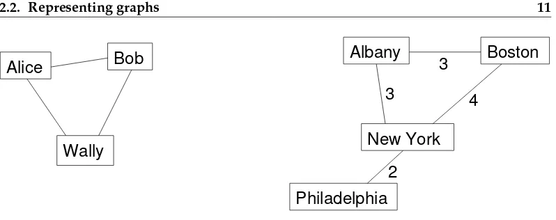
Figure 2.1: Examples of graphs.

2.2

Representing graphs

Graphs are usually drawn with squares or circles for nodes and lines for edges. In the example below, the graph on the left represents a social network with three people. In the graph on the right, the weights of the edges are the approximate travel times, in hours, between cities in the northeast United States. In this case the placement of the nodes corresponds roughly to the geography of the cities, but in general the layout of a graph is arbitrary.

To implement graph algorithms, you have to figure out how to represent a graph in the form of a data structure. But to choose the best data structure, you have to know which operations the graph should support.

To get out of this chicken-and-egg problem, I am going to present a data structure that is a good choice for many graph algorithms. Later we will come back and evaluate its pros and cons.

Here is an implementation of a graph as a dictionary of dictionaries:

❝❧❛ss ●r❛♣❤✭❞✐❝t✮✿

❞❡❢ ❴❴✐♥✐t❴❴✭s❡❧❢✱ ✈s❂❬❪✱ ❡s❂❬❪✮✿

✧✧✧❝r❡❛t❡ ❛ ♥❡✇ ❣r❛♣❤✳ ✭✈s✮ ✐s ❛ ❧✐st ♦❢ ✈❡rt✐❝❡s❀ ✭❡s✮ ✐s ❛ ❧✐st ♦❢ ❡❞❣❡s✳✧✧✧

❢♦r ✈ ✐♥ ✈s✿

s❡❧❢✳❛❞❞❴✈❡rt❡①✭✈✮

❢♦r ❡ ✐♥ ❡s✿

s❡❧❢✳❛❞❞❴❡❞❣❡✭❡✮

❞❡❢ ❛❞❞❴✈❡rt❡①✭s❡❧❢✱ ✈✮✿ ✧✧✧❛❞❞ ✭✈✮ t♦ t❤❡ ❣r❛♣❤✧✧✧ s❡❧❢❬✈❪ ❂ ④⑥

❞❡❢ ❛❞❞❴❡❞❣❡✭s❡❧❢✱ ❡✮✿

(26)

■❢ t❤❡r❡ ✐s ❛❧r❡❛❞② ❛♥ ❡❞❣❡ ❝♦♥♥❡❝t✐♥❣ t❤❡s❡ ❱❡rt✐❝❡s✱ t❤❡ ♥❡✇ ❡❞❣❡ r❡♣❧❛❝❡s ✐t✳

✧✧✧ ✈✱ ✇ ❂ ❡ s❡❧❢❬✈❪❬✇❪ ❂ ❡ s❡❧❢❬✇❪❬✈❪ ❂ ❡

The first line declares that●r❛♣❤inherits from the built-in type❞✐❝t, so a Graph object has all the methods and operators of a dictionary.

More specifically, a Graph is a dictionary that maps from a Vertexvto an inner dictionary that maps from a Vertexwto an Edge that connectsv andw. So if❣is a graph,❣❬✈❪❬✇❪ maps to an Edge if there is one and raises a❑❡②❊rr♦rotherwise.

❴❴✐♥✐t❴❴takes a list of vertices and a list of edges as optional parameters. If they are provided, it calls❛❞❞❴✈❡rt❡①and❛❞❞❴❡❞❣❡to add the vertices and edges to the graph. Adding a vertex to a graph means making an entry for it in the outer dictionary. Adding an edge makes two entries, both pointing to the same Edge. So this implementation represents an undirected graph.

Here is the definition for❱❡rt❡①:

❝❧❛ss ❱❡rt❡①✭♦❜❥❡❝t✮✿

❞❡❢ ❴❴✐♥✐t❴❴✭s❡❧❢✱ ❧❛❜❡❧❂✬✬✮✿ s❡❧❢✳❧❛❜❡❧ ❂ ❧❛❜❡❧

❞❡❢ ❴❴r❡♣r❴❴✭s❡❧❢✮✿

r❡t✉r♥ ✬❱❡rt❡①✭✪s✮✬ ✪ r❡♣r✭s❡❧❢✳❧❛❜❡❧✮

❴❴str❴❴ ❂ ❴❴r❡♣r❴❴

A Vertex is just an object that has a label attribute. We can add attributes later, as needed.

❴❴r❡♣r❴❴is a special function that returns a string representation of an object. It is similar to❴❴str❴❴except that the return value from❴❴str❴❴is intended to be readable for people, and the return value from❴❴r❡♣r❴❴is supposed to be a legal Python expression.

The built-in functionstrinvokes❴❴str❴❴on an object; similarly the built-in functionr❡♣r invokes❴❴r❡♣r❴❴.

In this case❱❡rt❡①✳❴❴str❴❴and ❱❡rt❡①✳❴❴r❡♣r❴❴refer to the same function, so we get the same string either way.

Here is the definition for❊❞❣❡:

❝❧❛ss ❊❞❣❡✭t✉♣❧❡✮✿

❞❡❢ ❴❴♥❡✇❴❴✭❝❧s✱ ✯✈s✮✿

r❡t✉r♥ t✉♣❧❡✳❴❴♥❡✇❴❴✭❝❧s✱ ✈s✮

(27)

2.2. Representing graphs 13

r❡t✉r♥ ✬❊❞❣❡✭✪s✱ ✪s✮✬ ✪ ✭r❡♣r✭s❡❧❢❬✵❪✮✱ r❡♣r✭s❡❧❢❬✶❪✮✮

❴❴str❴❴ ❂ ❴❴r❡♣r❴❴

❊❞❣❡ inherits from the built-in type t✉♣❧❡ and overrides the ❴❴♥❡✇❴❴ method. When you invoke an object constructor, Python invokes ❴❴♥❡✇❴❴to create the object and then

❴❴✐♥✐t❴❴to initialize the attributes.

For mutable objects it is most common to override ❴❴✐♥✐t❴❴and use the default imple-mentation of❴❴♥❡✇❴❴, but because Edges inherit fromt✉♣❧❡, they are immutable, which means that you can’t modify the elements of the tuple in❴❴✐♥✐t❴❴.

By overriding❴❴♥❡✇❴❴, we can use the✯operator to gather the parameters and use them to initialize the elements of the tuple. A precondition of this method is that there should be exactly two arguments. A more careful implementation would check.

Here is an example that creates two vertices and an edge:

✈ ❂ ❱❡rt❡①✭✬✈✬✮ ✇ ❂ ❱❡rt❡①✭✬✇✬✮ ❡ ❂ ❊❞❣❡✭✈✱ ✇✮ ♣r✐♥t ❡

Inside❊❞❣❡✳❴❴str❴❴the terms❡❧❢❬✵❪refers to✈ands❡❧❢❬✶❪refers to✇. So the output when you print❡is:

❊❞❣❡✭❱❡rt❡①✭✬✈✬✮✱ ❱❡rt❡①✭✬✇✬✮✮

Now we can assemble the edge and vertices into a graph:

❣ ❂ ●r❛♣❤✭❬✈✱ ✇❪✱ ❬❡❪✮ ♣r✐♥t ❣

The output looks like this (with a little formatting):

④❱❡rt❡①✭✬✇✬✮✿ ④❱❡rt❡①✭✬✈✬✮✿ ❊❞❣❡✭❱❡rt❡①✭✬✈✬✮✱ ❱❡rt❡①✭✬✇✬✮✮⑥✱ ❱❡rt❡①✭✬✈✬✮✿ ④❱❡rt❡①✭✬✇✬✮✿ ❊❞❣❡✭❱❡rt❡①✭✬✈✬✮✱ ❱❡rt❡①✭✬✇✬✮✮⑥⑥

We didn’t have to write●r❛♣❤✳❴❴str❴❴; it is inherited from❞✐❝t.

Exercise 2.2. In this exercise you write methods that will be useful for many of the Graph algo-rithms that are coming up.

1. Downloadt❤✐♥❦❝♦♠♣❧❡①✳ ❝♦♠✴ ●r❛♣❤❈♦❞❡✳ ♣②, which contains the code in this chapter. Run it as a script and make sure the test code in♠❛✐♥does what you expect.

2. Make a copy of ●r❛♣❤❈♦❞❡✳♣② called ●r❛♣❤✳♣②. Add the following methods to●r❛♣❤, adding test code as you go.

3. Write a method named❣❡t❴❡❞❣❡that takes two vertices and returns the edge between them if it exists and◆♦♥❡otherwise. Hint: use atr②statement.

(28)

5. Write a method named✈❡rt✐❝❡sthat returns a list of the vertices in a graph.

6. Write a method named❡❞❣❡sthat returns a list of edges in a graph. Note that in our repre-sentation of an undirected graph there are two references to each edge.

7. Write a method named♦✉t❴✈❡rt✐❝❡sthat takes a Vertex and returns a list of the adjacent vertices (the ones connected to the given node by an edge).

8. Write a method named♦✉t❴❡❞❣❡sthat takes a Vertex and returns a list of edges connected to the given Vertex.

9. Write a method named ❛❞❞❴❛❧❧❴❡❞❣❡s that starts with an edgeless Graph and makes a complete graph by adding edges between all pairs of vertices.

Test your methods by writing test code and checking the output. Then downloadt❤✐♥❦❝♦♠♣❧❡①✳

❝♦♠✴ ●r❛♣❤❲♦r❧❞✳ ♣②. GraphWorld is a simple tool for generating visual representations of graphs. It is based on the World class in Swampy, so you might have to install Swampy first: seet❤✐♥❦♣②t❤♦♥✳ ❝♦♠✴ s✇❛♠♣②.

Read through●r❛♣❤❲♦r❧❞✳♣②to get a sense of how it works. Then run it. It should import your

●r❛♣❤✳♣②and then display a complete graph with 10 vertices.

Exercise 2.3. Write a method named❛❞❞❴r❡❣✉❧❛r❴❡❞❣❡sthat starts with an edgeless graph and adds edges so that every vertex has the same degree. Thedegreeof a node is the number of edges it is connected to.

To create a regular graph with degree 2 you would do something like this:

✈❡rt✐❝❡s ❂ ❬ ✳✳✳ ❧✐st ♦❢ ❱❡rt✐❝❡s ✳✳✳ ❪ ❣ ❂ ●r❛♣❤✭✈❡rt✐❝❡s✱ ❬❪✮

❣✳❛❞❞❴r❡❣✉❧❛r❴❡❞❣❡s✭✷✮

It is not always possible to create a regular graph with a given degree, so you should figure out and document the preconditions for this method.

To test your code, you might want to create a file named●r❛♣❤❚❡st✳♣②that imports●r❛♣❤✳♣② and●r❛♣❤❲♦r❧❞✳♣②, then generates and displays the graphs you want to test.

2.3

Random graphs

A random graph is just what it sounds like: a graph with edges generated at random. Of course, there are many random processes that can generate graphs, so there are many kinds of random graphs. One interesting kind is the Erd˝os-Rényi model, denotedG(n,p), which generates graphs withnnodes, where the probability is p that there is an edge between any two nodes. See❤tt♣✿✴✴❡♥✳✇✐❦✐♣❡❞✐❛✳♦r❣✴✇✐❦✐✴❊r❞♦s✲❘❡♥②✐❴♠♦❞❡❧.

(29)

2.4. Connected graphs 15

2.4

Connected graphs

A graph isconnectedif there is a path from every node to every other node. See❤tt♣✿

✴✴❡♥✳✇✐❦✐♣❡❞✐❛✳♦r❣✴✇✐❦✐✴❈♦♥♥❡❝t✐✈✐t②❴✭❣r❛♣❤❴t❤❡♦r②✮.

There is a simple algorithm to check whether a graph is connected. Start at any vertex and conduct a search (usually a breadth-first-search or BFS), marking all the vertices you can reach. Then check to see whether all vertices are marked.

You can read about breadth-first-search at ❤tt♣✿✴✴❡♥✳✇✐❦✐♣❡❞✐❛✳♦r❣✴✇✐❦✐✴

❇r❡❛❞t❤✲❢✐rst❴s❡❛r❝❤.

In general, when you process a node, we say that you arevisitingit.

In a search, you visit a node by marking it (so you can tell later that it has been visited) then visiting any unmarked vertices it is connected to.

In a breadth-first-search, you visit nodes in the order they are discovered. You can use a queue or a “worklist” to keep them in order. Here’s how it works:

1. Start with any vertex and add it to the queue.

2. Remove a vertex from the queue and mark it. If it is connected to any unmarked vertices, add them to the queue.

3. If the queue is not empty, go back to Step 2.

Exercise 2.5. Write a Graph method named ✐s❴❝♦♥♥❡❝t❡❞ that returns ❚r✉❡ if the Graph is connected and❋❛❧s❡otherwise.

2.5

Paul Erd ˝os: peripatetic mathematician, speed freak

Paul Erd˝os was a Hungarian mathematician who spent most of his career (from 1934 until his death in 1992) living out of a suitcase, visiting colleagues at universities all over the world, and authoring papers with more than 500 collaborators.

He was a notorious caffeine addict and, for the last 20 years of his life, an enthusiastic user of amphetamines. He attributed at least some of his productivity to the use of these drugs; after giving them up for a month to win a bet, he complained that the only result was that mathematics had been set back by a month1.

In the 1960s he and Afréd Rényi wrote a series of papers introducing the Erd˝os-Rényi model of random graphs and studying their properties. The second is available from❤tt♣✿✴✴✇✇✇✳r❡♥②✐✳❤✉✴⑦♣❴❡r❞♦s✴✶✾✻✵✲✶✵✳♣❞❢.

One of their most surprising results is the existence of abrupt changes in the characteristics of random graphs as random edges are added. They showed that for a number of graph properties there is a threshold value of the probabilitypbelow which is the property is rare and above which it is almost certain. This transition is sometimes called a “phase change” by analogy with physical systems that change state at some critical value of temperature. See❤tt♣✿✴✴❡♥✳✇✐❦✐♣❡❞✐❛✳♦r❣✴✇✐❦✐✴P❤❛s❡❴tr❛♥s✐t✐♦♥.

(30)

Exercise 2.6. One of the properties that displays this kind of transition is connectedness. For a given size n, there is a critical value, p∗, such that a random graph G(n,p) is unlikely to be connected if p<_p∗_{and very likely to be connected if p}> _p∗_.

Write a program that tests this result by generating random graphs for values of n and p and computes the fraction of them that are connected.

How does the abruptness of the transition depend on n?

You can download my solution fromt❤✐♥❦❝♦♠♣❧❡①✳ ❝♦♠✴ ❘❛♥❞♦♠●r❛♣❤✳ ♣②.

2.6

Iterators

If you have read the documentation of Python dictionaries, you might have noticed the methods✐t❡r❦❡②s,✐t❡r✈❛❧✉❡sand✐t❡r✐t❡♠s. These methods are similar to❦❡②s,✈❛❧✉❡s and✐t❡♠s, except that instead of building a new list, they return iterators.

Aniteratoris an object that provides a method named♥❡①tthat returns the next element in a sequence. Here is an example that creates a dictionary and uses✐t❡r❦❡②sto traverse the keys.

❃❃❃ ❞ ❂ ❞✐❝t✭❛❂✶✱ ❜❂✷✮ ❃❃❃ ✐t❡r ❂ ❞✳✐t❡r❦❡②s✭✮ ❃❃❃ ♣r✐♥t ✐t❡r✳♥❡①t✭✮ ❛

❃❃❃ ♣r✐♥t ✐t❡r✳♥❡①t✭✮ ❜

❃❃❃ ♣r✐♥t ✐t❡r✳♥❡①t✭✮

❚r❛❝❡❜❛❝❦ ✭♠♦st r❡❝❡♥t ❝❛❧❧ ❧❛st✮✿ ❋✐❧❡ ✧❁st❞✐♥❃✧✱ ❧✐♥❡ ✶✱ ✐♥ ❁♠♦❞✉❧❡❃ ❙t♦♣■t❡r❛t✐♦♥

The first time♥❡①tis invoked, it returns the first key from the dictionary (the order of the keys is arbitrary). The second time it is invoked, it returns the second element. The third time, and every time thereafter, it raises a❙t♦♣■t❡r❛t✐♦♥exception.

An iterator can be used in a❢♦rloop; for example, the following is a common idiom for traversing the key-value pairs in a dictionary:

❢♦r ❦✱ ✈ ✐♥ ❞✳✐t❡r✐t❡♠s✭✮✿ ♣r✐♥t ❦✱ ✈

In this context,✐t❡r✐t❡♠sis likely to be faster than✐t❡♠sbecause it doesn’t have to build the entire list of tuples; it reads them from the dictionary as it goes along.

But it is only safe to use the iterator methods if you do not add or remove dictionary keys inside the loop. Otherwise you get an exception:

❃❃❃ ❞ ❂ ❞✐❝t✭❛❂✶✮

❃❃❃ ❢♦r ❦ ✐♥ ❞✳✐t❡r❦❡②s✭✮✿

(31)

2.7. Generators 17

✳✳✳

❘✉♥t✐♠❡❊rr♦r✿ ❞✐❝t✐♦♥❛r② ❝❤❛♥❣❡❞ s✐③❡ ❞✉r✐♥❣ ✐t❡r❛t✐♦♥

Another limitation of iterators is that they do not support index operations.

❃❃❃ ✐t❡r ❂ ❞✳✐t❡r❦❡②s✭✮ ❃❃❃ ♣r✐♥t ✐t❡r❬✶❪

❚②♣❡❊rr♦r✿ ✬❞✐❝t✐♦♥❛r②✲❦❡②✐t❡r❛t♦r✬ ♦❜❥❡❝t ✐s ✉♥s✉❜s❝r✐♣t❛❜❧❡

If you need indexed access, you should use ❦❡②s. Alternatively, the Python module

✐t❡rt♦♦❧sprovides many useful iterator functions.

A user-defined object can be used as an iterator if it provides methods named ♥❡①tand

❴❴✐t❡r❴❴. The following example is an iterator that always returns❚r✉❡:

❝❧❛ss ❆❧❧❚r✉❡✭♦❜❥❡❝t✮✿ ❞❡❢ ♥❡①t✭s❡❧❢✮✿

r❡t✉r♥ ❚r✉❡

❞❡❢ ❴❴✐t❡r❴❴✭s❡❧❢✮✿ r❡t✉r♥ s❡❧❢

The❴❴✐t❡r❴❴method for iterators returns the iterator itself. This protocol makes it possible to use iterators and sequences interchangeably in many contexts.

Iterators like❆❧❧❚r✉❡can represent an infinite sequence. They are useful as an argument to③✐♣:

❃❃❃ ♣r✐♥t ③✐♣✭✬❛❜❝✬✱ ❆❧❧❚r✉❡✭✮✮

❬✭✬❛✬✱ ❚r✉❡✮✱ ✭✬❜✬✱ ❚r✉❡✮✱ ✭✬❝✬✱ ❚r✉❡✮❪

2.7

Generators

For many purposes the easiest way to make an iterator is to write agenerator, which is a function that contains a②✐❡❧❞statement. ②✐❡❧❞is similar tor❡t✉r♥, except that the state of the running function is stored and can be resumed.

For example, here is a generator that yields successive letters of the alphabet:

❞❡❢ ❣❡♥❡r❛t❡❴❧❡tt❡rs✭✮✿ ❢♦r ❧❡tt❡r ✐♥ ✬❛❜❝✬✿

②✐❡❧❞ ❧❡tt❡r

When you call this function, the return value is an iterator:

❃❃❃ ✐t❡r ❂ ❣❡♥❡r❛t❡❴❧❡tt❡rs✭✮ ❃❃❃ ♣r✐♥t ✐t❡r

❁❣❡♥❡r❛t♦r ♦❜❥❡❝t ❛t ✵①❜✼❞✹❝❡✹❝❃ ❃❃❃ ♣r✐♥t ✐t❡r✳♥❡①t✭✮

❛

(32)

And you can use an iterator in a❢♦rloop:

❃❃❃ ❢♦r ❧❡tt❡r ✐♥ ❣❡♥❡r❛t❡❴❧❡tt❡rs✭✮✿

✳✳✳ ♣r✐♥t ❧❡tt❡r

✳✳✳ ❛ ❜ ❝

A generator with an infinite loop returns an iterator that never terminates. For example, here’s a generator that cycles through the letters of the alphabet:

❞❡❢ ❛❧♣❤❛❜❡t❴❝②❝❧❡✭✮✿ ✇❤✐❧❡ ❚r✉❡✿

❢♦r ❝ ✐♥ str✐♥❣✳❧♦✇❡r❝❛s❡✿ ②✐❡❧❞ ❝

(33)

Chapter 3

Analysis of algorithms

Analysis of algorithms is the branch of computer science that studies the performance of algorithms, especially their run time and space requirements. See❤tt♣✿✴✴❡♥✳✇✐❦✐♣❡❞✐❛✳

♦r❣✴✇✐❦✐✴❆♥❛❧②s✐s❴♦❢❴❛❧❣♦r✐t❤♠s.

The practical goal of algorithm analysis is to predict the performance of different algo-rithms in order to guide design decisions.

During the 2008 United States Presidential Campaign, candidate Barack Obama was asked to perform an impromptu analysis when he visited Google. Chief executive Eric Schmidt jokingly asked him for “the most efficient way to sort a million 32-bit integers.” Obama had apparently been tipped off, because he quickly replied, “I think the bubble sort would be the wrong way to go.” See❤tt♣✿✴✴✇✇✇✳②♦✉t✉❜❡✳❝♦♠✴✇❛t❝❤❄✈❂❦✹❘❘✐❴♥t◗❝✽.

This is true: bubble sort is conceptually simple but slow for large datasets. The answer Schmidt was probably looking for is “radix sort” (see ❤tt♣✿✴✴❡♥✳✇✐❦✐♣❡❞✐❛✳♦r❣✴✇✐❦✐✴

❘❛❞✐①❴s♦rt)1_.

So the goal of algorithm analysis is to make meaningful comparisons between algorithms, but there are some problems:

• The relative performance of the algorithms might depend on characteristics of the hardware, so one algorithm might be faster on Machine A, another on Machine B. The general solution to this problem is to specify amachine modeland analyze the number of steps, or operations, an algorithm requires under a given model.

• Relative performance might depend on the details of the dataset. For example, some sorting algorithms run faster if the data are already partially sorted; other algorithms run slower in this case. A common way to avoid this problem is to analyze theworst casescenario. It is also sometimes useful to analyze average case performance, but it is usually harder, and sometimes it is not clear what set of cases to average over.

1_{But if you get a question like this in an interview, I think a better answer is, “The fastest way to sort a million}

(34)

• Relative performance also depends on the size of the problem. A sorting algorithm that is fast for small lists might be slow for long lists. The usual solution to this problem is to express run time (or number of operations) as a function of problem size, and to compare the functionsasymptoticallyas the problem size increases. The good thing about this kind of comparison that it lends itself to simple classification of algorithms. For example, if I know that the run time of Algorithm A tends to be propor-tional to the size of the input,n, and Algorithm B tends to be proportional ton2, then I expect A to be faster than B for large values ofn.

This kind of analysis comes with some caveats, but we’ll get to that later.

3.1

Order of growth

Suppose you have analyzed two algorithms and expressed their run times in terms of the size of the input: Algorithm A takes 100n+1 steps to solve a problem with sizen; Algo-rithm B takesn2₊_n₊_{1 steps.}

The following table shows the run time of these algorithms for different problem sizes: Input Run time of Run time of

size Algorithm A Algorithm B

10 1 001 111

100 10 001 10 101

1 000 100 001 1 001 001

10 000 1 000 001 >1010

Atn =10, Algorithm A looks pretty bad; it takes almost 10 times longer than Algorithm B. But forn=100 they are about the same, and for larger values A is much better.

The fundamental reason is that for large values ofn, any function that contains ann2term will grow faster than a function whose leading term isn. Theleading termis the term with the highest exponent.

For Algorithm A, the leading term has a large coefficient, 100, which is why B does better than A for smalln. But regardless of the coefficients, there will always be some value ofn

wherean2>bn.

The same argument applies to the non-leading terms. Even if the run time of Algorithm A weren+1000000, it would still be better than Algorithm B for sufficiently largen.

In general, we expect an algorithm with a smaller leading term to be a better algorithm for large problems, but for smaller problems, there may be acrossover pointwhere another algorithm is better. The location of the crossover point depends on the details of the algo-rithms, the inputs, and the hardware, so it is usually ignored for purposes of algorithmic analysis. But that doesn’t mean you can forget about it.

(35)

3.1. Order of growth 21

Anorder of growthis a set of functions whose asymptotic growth behavior is considered equivalent. For example, 2n, 100nandn+1 belong to the same order of growth, which is writtenO(n)inBig-Oh notationand often calledlinearbecause every function in the set grows linearly withn.

All functions with the leading termn2belong toO(n2); they arequadratic, which is a fancy word for functions with the leading termn2.

The following table shows some of the orders of growth that appear most commonly in algorithmic analysis, in increasing order of badness.

Order of Name

growth

O(1) constant

O(log_bn) logarithmic (for anyb)

O(n) linear

O(nlog_bn) “en log en”

O(n2) quadratic

O(n3) cubic

O(cn) exponential (for anyc)

For the logarithmic terms, the base of the logarithm doesn’t matter; changing bases is the equivalent of multiplying by a constant, which doesn’t change the order of growth. Sim-ilarly, all exponential functions belong to the same order of growth regardless of the base of the exponent. Exponential functions grow very quickly, so exponential algorithms are only useful for small problems.

Exercise 3.1. Read the Wikipedia page on Big-Oh notation at ❤tt♣✿ ✴✴ ❡♥✳ ✇✐❦✐♣❡❞✐❛✳ ♦r❣✴

✇✐❦✐✴ ❇✐❣❴ ❖❴ ♥♦t❛t✐♦♥ and answer the following questions:

1. What is the order of growth of n3+n2? What about1000000n3+n2? What about n3+ 1000000n2?

2. What is the order of growth of(n2+n)·(n+1)? Before you start multiplying, remember that you only need the leading term.

3. If f is in O(g), for some unspecified function g, what can we say about a f+b?

4. If f1and f2are in O(g), what can we say about f1+f2?

5. If f₁is in O(g)and f2is in O(h), what can we say about f1+f2?

6. If f1is in O(g)and f2is O(h), what can we say about f1∗f2?

Programmers who care about performance often find this kind of analysis hard to swal-low. They have a point: sometimes the coefficients and the non-leading terms make a real difference. And sometimes the details of the hardware, the programming language, and the characteristics of the input make a big difference. And for small problems asymptotic behavior is irrelevant.

(36)

3.2

Analysis of basic operations

Most arithmetic operations are constant time; multiplication usually takes longer than ad-dition and subtraction, and division takes even longer, but these run times don’t depend on the magnitude of the operands. Very large integers are an exception; in that case the run time increases linearly with the number of digits.

Indexing operations—reading or writing elements in a sequence or dictionary—are also constant time, regardless of the size of the data structure.

A❢♦r loop that traverses a sequence or dictionary is usually linear, as long as all of the operations in the body of the loop are constant time. For example, adding up the elements of a list is linear:

t♦t❛❧ ❂ ✵ ❢♦r ① ✐♥ t✿

t♦t❛❧ ✰❂ ①

The built-in functions✉♠is also linear because it does the same thing, but it tends to be faster because it is a more efficient implementation; in the language of algorithmic analysis, it has a smaller leading coefficient.

If you use the same loop to “add” a list of strings, the run time is quadratic because string concatenation is linear.

The string method❥♦✐♥is usually faster because it is linear in the total length of the strings.

As a rule of thumb, if the body of a loop is inO(na)then the whole loop is inO(na+1). The exception is if you can show that the loop exits after a constant number of iterations. If a loop runsktimes regardless ofn, then the loop is inO(na), even for largek.

Multiplying bykdoesn’t change the order of growth, but neither does dividing. So if the body of a loop is inO(na)and it runsn/ktimes, the loop is inO(na+1), even for largek. Most string and tuple operations are linear, except indexing and❧❡♥, which are constant time. The built-in functions♠✐♥ and♠❛① are linear. The run-time of a slice operation is proportional to the length of the output, but independent of the size of the input.

All string methods are linear, but if the lengths of the strings are bounded by a constant— for example, operations on single characters—they are considered constant time.

Most list methods are linear, but there are some exceptions:

• Adding an element to the end of a list is constant time on average; when it runs out of room it occasionally gets copied to a bigger location, but the total time forn

operations isO(n), so we say that the “amortized” time for one operation isO(1). • Removing an element from the end of a list is constant time.

• Sorting isO(nlogn).

(37)

3.3. Analysis of search algorithms 23

• The run time of❝♦♣②is proportional to the number of elements, but not the size of the elements (it copies references, not the elements themselves).

• The run time of✉♣❞❛t❡is proportional to the size of the dictionary passed as a pa-rameter, not the dictionary being updated.

• ❦❡②s, ✈❛❧✉❡s and ✐t❡♠s are linear because they return new lists; ✐t❡r❦❡②s,

✐t❡r✈❛❧✉❡s and✐t❡r✐t❡♠s are constant time because they return iterators. But if you loop through the iterators, the loop will be linear. Using the “iter” functions saves some overhead, but it doesn’t change the order of growth unless the number of items you access is bounded.

The performance of dictionaries is one of the minor miracles of computer science. We will see how they work in Section 3.4.

Exercise 3.2. Read the Wikipedia page on sorting algorithms at❤tt♣✿ ✴✴ ❡♥✳ ✇✐❦✐♣❡❞✐❛✳ ♦r❣✴

✇✐❦✐✴ ❙♦rt✐♥❣❴ ❛❧❣♦r✐t❤♠ and answer the following questions:

1. What is a “comparison sort?” What is the best worst-case order of growth for a comparison sort? What is the best worst-case order of growth for any sort algorithm?

2. What is the order of growth of bubble sort, and why does Barack Obama think it is “the wrong way to go?”

3. What is the order of growth of radix sort? What preconditions do we need to use it?

4. What is a stable sort and why might it matter in practice?

5. What is the worst sorting algorithm (that has a name)?

6. What sort algorithm does the C library use? What sort algorithm does Python use? Are these algorithms stable? You might have to Google around to find these answers.

7. Many of the non-comparison sorts are linear, so why does does Python use an O(nlogn)

comparison sort?

3.3

Analysis of search algorithms

Asearchis an algorithm that takes a collection and a target item and determines whether the target is in the collection, often returning the index of the target.

The simplest search algorithm is a “linear search,” which traverses the items of the collec-tion in order, stopping if it finds the target. In the worst case it has to traverse the entire collection, so the run time is linear.

The ✐♥operator for sequences uses a linear search; so do string methods like❢✐♥❞ and

❝♦✉♥t.

If the elements of the sequence are in order, you can use a bisection search, which is

(38)

the word you are looking for comes before or after. If it comes before, then you search the first half of the sequence. Otherwise you search the second half. Either way, you cut the number of remaining items in half.

If the sequence has 1,000,000 items, it will take about 20 steps to find the word or conclude that it’s not there. So that’s about 50,000 times faster than a linear search.

Exercise 3.3. Write a function called❜✐s❡❝t✐♦♥ that takes a sorted list and a target value and returns the index of the value in the list, if it’s there, or◆♦♥❡if it’s not.

Or you could read the documentation of the❜✐s❡❝tmodule and use that!

Bisection search can be much faster than linear search, but it requires the sequence to be in order, which might require extra work.

There is another data structure, called ahashtablethat is even faster—it can do a search in constant time—and it doesn’t require the items to be sorted. Python dictionaries are implemented using hashtables, which is why most dictionary operations, including the✐♥ operator, are constant time.

3.4

Hashtables

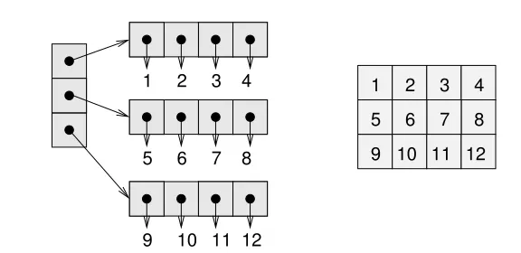
To explain how hashtables work and why their performance is so good, I start with a simple implementation of a map and gradually improve it until it’s a hashtable.

I use Python to demonstrate these implementations, but in real life you wouldn’t write code like this in Python; you would just use a dictionary! So for the rest of this chapter, you have to imagine that dictionaries don’t exist and you want to implement a data structure that maps from keys to values. The operations you have to implement are:

❛❞❞✭❦✱ ✈✮: Add a new item that maps from key❦to value✈. With a Python dictionary,❞, this operation is written❞❬❦❪ ❂ ✈.

❣❡t✭t❛r❣❡t✮: Look up and return the value that corresponds to keyt❛r❣❡t. With a Python dictionary,❞, this operation is written❞❬t❛r❣❡t❪or❞✳❣❡t✭t❛r❣❡t✮.

For now, I assume that each key only appears once. The simplest implementation of this interface uses a list of tuples, where each tuple is a key-value pair.

❝❧❛ss ▲✐♥❡❛r▼❛♣✭♦❜❥❡❝t✮✿

❞❡❢ ❴❴✐♥✐t❴❴✭s❡❧❢✮✿ s❡❧❢✳✐t❡♠s ❂ ❬❪

❞❡❢ ❛❞❞✭s❡❧❢✱ ❦✱ ✈✮✿

s❡❧❢✳✐t❡♠s✳❛♣♣❡♥❞✭✭❦✱ ✈✮✮

❞❡❢ ❣❡t✭s❡❧❢✱ ❦✮✿

❢♦r ❦❡②✱ ✈❛❧ ✐♥ s❡❧❢✳✐t❡♠s✿ ✐❢ ❦❡② ❂❂ ❦✿

(39)

3.4. Hashtables 25

❛❞❞appends a key-value tuple to the list of items, which takes constant time.

❣❡tuses a❢♦rloop to search the list: if it finds the target key it returns the corresponding value; otherwise it raises a❑❡②❊rr♦r. So❣❡tis linear.

An alternative is to keep the list sorted by key. Then ❣❡t could use a bisection search, which isO(logn). But inserting a new item in the middle of a list is linear, so this might not be the best option. There are other data structures (see❤tt♣✿✴✴❡♥✳✇✐❦✐♣❡❞✐❛✳♦r❣✴

✇✐❦✐✴❘❡❞✲❜❧❛❝❦❴tr❡❡) that can implement❛❞❞and❣❡tin log time, but that’s still not as good as a hashtable, so let’s move on.

One way to improve ▲✐♥❡❛r▼❛♣ is to break the list of key-value pairs into smaller lists. Here’s an implementation called ❇❡tt❡r▼❛♣, which is a list of 100 LinearMaps. As we’ll see in a second, the order of growth for ❣❡tis still linear, but❇❡tt❡r▼❛♣is a step on the path toward hashtables:

❝❧❛ss ❇❡tt❡r▼❛♣✭♦❜❥❡❝t✮✿

❞❡❢ ❴❴✐♥✐t❴❴✭s❡❧❢✱ ♥❂✶✵✵✮✿ s❡❧❢✳♠❛♣s ❂ ❬❪

❢♦r ✐ ✐♥ r❛♥❣❡✭♥✮✿

s❡❧❢✳♠❛♣s✳❛♣♣❡♥❞✭▲✐♥❡❛r▼❛♣✭✮✮

❞❡❢ ❢✐♥❞❴♠❛♣✭s❡❧❢✱ ❦✮✿

✐♥❞❡① ❂ ❤❛s❤✭❦✮ ✪ ❧❡♥✭s❡❧❢✳♠❛♣s✮ r❡t✉r♥ s❡❧❢✳♠❛♣s❬✐♥❞❡①❪

❞❡❢ ❛❞❞✭s❡❧❢✱ ❦✱ ✈✮✿ ♠ ❂ s❡❧❢✳❢✐♥❞❴♠❛♣✭❦✮ ♠✳❛❞❞✭❦✱ ✈✮

❞❡❢ ❣❡t✭s❡❧❢✱ ❦✮✿

♠ ❂ s❡❧❢✳❢✐♥❞❴♠❛♣✭❦✮ r❡t✉r♥ ♠✳❣❡t✭❦✮

❴❴✐♥✐t❴❴makes a list of♥ ▲✐♥❡❛r▼❛♣s.

❢✐♥❞❴♠❛♣is used by❛❞❞and❣❡tto figure out which map to put the new item in, or which map to search.

❢✐♥❞❴♠❛♣uses the built-in function❤❛s❤, which takes almost any Python object and returns an integer. A limitation of this implementation is that it only works with hashable keys. Mutable types like lists and dictionaries are unhashable.

Hashable objects that are considered equal return the same hash value, but the converse is not necessarily true: two different objects can return the same hash value.

❢✐♥❞❴♠❛♣ uses the modulus operator to wrap the hash values into the range from 0 to

(40)

Since the run time of▲✐♥❡❛r▼❛♣✳❣❡tis proportional to the number of items, we expect BetterMap to be about 100 times faster than LinearMap. The order of growth is still linear, but the leading coefficient is smaller. That’s nice, but still not as good as a hashtable. Here (finally) is the crucial idea that makes hashtables fast: if you can keep the maximum length of the LinearMaps bounded,▲✐♥❡❛r▼❛♣✳❣❡tis constant time. All you have to do is keep track of the number of items and when the number of items per LinearMap exceeds a threshold, resize the hashtable by adding more LinearMaps.

Here is an implementation of a hashtable:

❝❧❛ss ❍❛s❤▼❛♣✭♦❜❥❡❝t✮✿

❞❡❢ ❴❴✐♥✐t❴❴✭s❡❧❢✮✿

s❡❧❢✳♠❛♣s ❂ ❇❡tt❡r▼❛♣✭✷✮ s❡❧❢✳♥✉♠ ❂ ✵

❞❡❢ ❣❡t✭s❡❧❢✱ ❦✮✿

r❡t✉r♥ s❡❧❢✳♠❛♣s✳❣❡t✭❦✮

❞❡❢ ❛❞❞✭s❡❧❢✱ ❦✱ ✈✮✿

✐❢ s❡❧❢✳♥✉♠ ❂❂ ❧❡♥✭s❡❧❢✳♠❛♣s✳♠❛♣s✮✿ s❡❧❢✳r❡s✐③❡✭✮

s❡❧❢✳♠❛♣s✳❛❞❞✭❦✱ ✈✮ s❡❧❢✳♥✉♠ ✰❂ ✶

❞❡❢ r❡s✐③❡✭s❡❧❢✮✿

♥❡✇❴♠❛♣s ❂ ❇❡tt❡r▼❛♣✭s❡❧❢✳♥✉♠ ✯ ✷✮

❢♦r ♠ ✐♥ s❡❧❢✳♠❛♣s✳♠❛♣s✿ ❢♦r ❦✱ ✈ ✐♥ ♠✳✐t❡♠s✿

♥❡✇❴♠❛♣s✳❛❞❞✭❦✱ ✈✮

Each❍❛s❤▼❛♣contains a❇❡tt❡r▼❛♣;❴❴✐♥✐t❴❴starts with just 2 LinearMaps and initializes

♥✉♠, which keeps track of the number of items.

❣❡tjust dispatches to❇❡tt❡r▼❛♣. The real work happens in❛❞❞, which checks the number of items and the size of the❇❡tt❡r▼❛♣: if they are equal, the average number of items per LinearMap is 1, so it callsr❡s✐③❡.

r❡s✐③❡make a new❇❡tt❡r▼❛♣, twice as big as the previous one, and then “rehashes” the items from the old map to the new.

Rehashing is necessary because changing the number of LinearMaps changes the denom-inator of the modulus operator in❢✐♥❞❴♠❛♣. That means that some objects that used to wrap into the same LinearMap will get split up (which is what we wanted, right?). Rehashing is linear, sor❡s✐③❡is linear, which might seem bad, since I promised that❛❞❞ would be constant time. But remember that we don’t have to resize every time, so❛❞❞is usually constant time and only occasionally linear. The total amount of work to run❛❞❞n

(41)

3.4. Hashtables 27

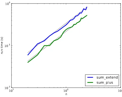
Figure 3.1: The cost of a hashtable add.

To see how this works, think about starting with an empty HashTable and adding a se-quence of items. We start with 2 LinearMaps, so the first 2 adds are fast (no resizing re-quired). Let’s say that they take one unit of work each. The next add requires a resize, so we have to rehash the first two items (let’s call that 2 more units of work) and then add the third item (one more unit). Adding the next item costs 1 unit, so the total so far is 6 units of work for 4 items.

The next❛❞❞costs 5 units, but the next three are only one unit each, so the total is 14 units for the first 8 adds.

The next❛❞❞costs 9 units, but then we can add 7 more before the next resize, so the total is 30 units for the first 16 adds.

After 32 adds, the total cost is 62 units, and I hope you are starting to see a pattern. Aftern

adds, wherenis a power of two, the total cost is 2n−2 units, so the average work per add is a little less than 2 units. Whennis a power of two, that’s the best case; for other values of

nthe average work is a little higher, but that’s not important. The important thing is that it is consta