ROAD AND ROADSIDE FEATURE EXTRACTION USING IMAGERY AND LIDAR
DATA FOR TRANSPORTATION OPERATION
S. Urala,b, J. Shana, M. A. Romeroa, A. Tarkoa
aLyles School of Civil Engineering, Purdue University, West Lafayette, IN, U.S.A.- [email protected] b
Dept. of Geomatics Engineering, Hacettepe University, 06800, Beytepe, Ankara, Turkey – [email protected]
Commission III, WG III/1; ICWG III/VII
KEY WORDS: Imagery, LiDAR, remote sensing, graph cuts, road extraction, transportation
ABSTRACT:
Transportation agencies require up-to-date, reliable, and feasibly acquired information on road geometry and features within proximity to the roads as input for evaluating and prioritizing new or improvement road projects. The information needed for a robust evaluation of road projects includes road centerline, width, and extent together with the average grade, cross-sections, and obstructions near the travelled way. Remote sensing is equipped with a large collection of data and well-established tools for acquiring the information and extracting aforementioned various road features at various levels and scopes. Even with many remote sensing data and methods available for road extraction, transportation operation requires more than the centerlines. Acquiring information that is spatially coherent at the operational level for the entire road system is challenging and needs multiple data sources to be integrated. In the presented study, we established a framework that used data from multiple sources, including one-foot resolution color infrared orthophotos, airborne LiDAR point clouds, and existing spatially non-accurate ancillary road networks. We were able to extract 90.25% of a total of 23.6 miles of road networks together with estimated road width, average grade along the road, and cross sections at specified intervals. Also, we have extracted buildings and vegetation within a predetermined proximity to the extracted road extent. 90.6% of 107 existing buildings were correctly identified with 31% false detection rate.
1. INTRODUCTION
There is abundant research focused on the extraction of roads, road networks, and their related environment and information. Scopes involved in existing literature span from land cover classification of road class to extracting road centerlines, from extracting road networks by exploiting semantic, contextual, topological relationships to road geometric modeling. Datasets utilized include high resolution satellite images, aerial photos, and LiDAR (Light Detection and Ranging), as well as ancillary data, like existing road networks as contextual aid. The range of algorithms employed is also vast. Transportation agencies greatly benefit from this research effort since they require up-to-date road information with highest possible geometric reliability to perform operational tasks.
Such operational needs would include the examination of all cross section elements: lane width, median, shoulder, clear zones, etc. Some of these elements may be readily available as part of an inventory database. However, some information such as embankment slopes and height, ditch dimensions, and obstructions near the travelled way may not be included in such databases. One potentially feasible way of acquiring the missing information is using remote sensing techniques.
Even though there are many remote sensing methods for road extraction, transportation operation requires more than the centerlines. Acquiring information that is coherent in space at the operational level is difficult and needs the integral use of multiple data sources. The information required for a robust project evaluation includes cross-section dimensions with side slopes, longitudinal grades along the road, boundaries of the right of way (strip of land administered by the road administration), and obstructions near the traveled way such as trees and large man-made structures. The requirement for spatial coherence, for example, arises from the fact that one
needs to identify the roadside areas with designed clear zones to extract the obstructions and estimate the slopes therein.
Ideally, it is possible to identify the clear zones via spatially accurate road network and information on the roadway such as the lane width and the number of lanes. However, road network datasets with planimetric accuracy that will allow such identifications, or spatially related lane information may not be available consistently for large road networks. In that case, the travelled way (and its centerline), and the roadside areas need to be extracted with geometric reliability via remote sensing to acquire all other related information.
We propose a framework for extracting abovementioned information to be employed within a robust project evaluation methodology using remote sensing datasets. We employ orthophotos and LiDAR point clouds for extracting the required features with sophisticated and operationally feasible remote sensing methods.
2. RELATED WORK
The wide range of literature on road extraction involves consideration of many aspects. Researchers focus on various problem definitions, use a variety of data sources, and apply methods spanning a large collection of algorithms. Mena (2003) and Mayer et. al. (2006) provide detailed reviews on the state-of-the-art on road extraction. Here, we will refer to part of the existing research in literature in order to highlight several important aspects.
requires different approaches than using single images. Apart from imagery, SAR (Gamba et. al., 2013; Hedman et. al., 2006) and LiDAR (Hu et. al., 2014; Yang et. al., 2013; Kumar et. al., 2013; Boyko and Funkhouser, 2011) data are also exploited for road extraction.
The main body of literature focuses on the extraction of the road centerlines either for identifying the road network or updating an existing one. Among them, a group of methods first determine the linear features on the image by using edge detection algorithms (Steger, 1998; Lacroix and Aceroy, 1998) and then identify the roads by evaluating the extracted lines by various criteria (Bacher and Mayer, 2005). Another way to determine the linear features is by using a semi-automatic approach. The road is tracked initiating from interactively or automatically selected seed points (Baumgartner et. al., 2002; Zhao et. al., 2002). Some of such methods employ active contour models for tracing the roads (Mayer et. al., 1997; Laptev et. al., 2000).
In a distinct track of algorithms, mathematical morphology is used to determine the roads (Soille and Pesaresi, 2002; Valero et. al., 2010; Naouai et. al., 2010; Mohammadzadeh et. al.; 2006; Amini et. al., 2002). Formal morphological operations are mostly utilized in a sequential manner to perform simplification, thinning, gap filling or noise removal for extracting the road centerlines. Initial classification of the roads from the images may be carried out using pixel-based or object oriented classification approaches. In an object-oriented approach, road segments are first determined then to be further evaluated (Zhang and Coulognier, 2006; Miao et. al., 2013).
Exploitation of the images at multiple scales is frequently considered as a contributing factor to the overall success of the road extraction process. Various implementations of scale-space processing are presented in Mayer et. al. (1997), Baumgartner et. al. (1999), Laptev et. al. (2000), Hinz and Baumgartner (2003), Naouai et. al. (2010). Information extracted at coarse scales are usually used to avoid the negative effects of obstacles and noise, e.g., shadows and vehicles on the roads. Most road extraction research concentrate on and suited for rural or semi-urban areas for extracting road centerlines while research targeting urban and suburban areas (Hinz and Baumgartner, 2003; Poullis, 2010; Das et. al., 2011; Shi et. al., 2014) are comparatively less but growing. The complexity of the road extraction problem requires the research to look into ways of using all available information to contribute to a better solution. Frequently, multiple input datasets are employed for road extraction.
3. STUDY AREA AND DATA
We selected a study area of approximately five by two miles in the Union township, Clinton County, IN, USA for implementing the proposed framework. The remote sensing datasets we used are the most recent ones available by the time of the study from the 2011-2013 Indiana Orthophotography, LiDAR and Elevation Project. The data we employed include one-foot resolution CIR (Color Infrared) orthophotos, LiDAR point clouds, and the LiDAR derived DEMs (Digital Elevation Model, bare ground model) at a resolution of five feet. We also generated a DSM (Digital Surface Model) and an nDSM (normalized DSM) using the LiDAR point clouds of the study area. We used the existing road network dataset acquired from INDOT (Indiana Department of Transformation) database to generate an approximate buffer around the road lines. This buffer is then used as a mask for limiting the amount of data
involved in the process to the parts of the datasets that are relevant.
4. METHODOLOGY
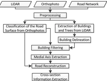
Our framework consists of multiple integral processes. First, there is a preprocessing step for preparing the datasets to be analyzed. Then, these datasets are employed in feature extraction, paved surface classification, medial axis extraction, paved surface reconstruction, and cross section information extraction processes. Figure 1 shows the overall flowchart for the framework.
Figure 1.Overall flowchart of the proposed framework
4.1. Classification of the Road Surface
4.1.1.Classification of the Paved Surface
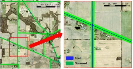
We applied SVM (Support Vector Machine) classifiers as part of a pixel based approach for the classification of the paved surface. SVM classification creates a maximum-margin hyper-plane in a transformed input space and splits the classes by maximizing the distance to the nearest clean split samples. This search for the optimal separating hyper-plane is performed after the original training data are transformed into a higher dimension. There is always a separating hyper-plane if the new dimension is sufficiently high and the transformation is appropriate. This hyper-plane is found with the aid of the “support vectors” (Han et. al., 2012). Details on SVMs may be found in Han et.al. (2012) or Theodoris and Koutroumbas (2009). We used a C-Support Vector Classification type of SVM with a linear kernel as implemented in ORFEO toolbox of CNES (2013). After training the SVM classifier, we classified the study area tile by tile using the same trained model for each tile. Classification results were then validated using randomly selected test samples. The confusion matrix for part of the dataset tested is provided in Table 1. An overall accuracy of 97.3% is achieved for road/non-road binary classification with a kappa value of 0.90. Figure 2 shows an example of the SVM classification result from part of the study area.
Non-road Road ∑
Table 1. Confusion matrix for road/non-road classification of CIR orthophotos. (P: Producer’s accuracy, U: User’s accuracy)
Figure 2. A sample from the road surface classification results
using SVM
4.1.2.Filtering Buildings
A very common misclassification that occurs while extracting the paved road surface by classifying CIR orthophotos is the classification of some of the buildings contagious to the roads due to their spectral similarity. Additional information is required to avoid such misclassification. Ideally, having up-to-date building outlines would be sufficient to exclude the buildings. However, such building databases are not commonly available. Hence, one needs to determine the building outlines to use them as a mask for acquiring just the road surfaces out of the classification result. Several options are available for this purpose. Using the nDSM as an additional source of information is one remedy. A common alternative approach is to employ NDVI (Normalized Difference Vegetation Index) to mask the nDSM so that only high objects that are not vegetation remain to be used to filter the image classification results. Both methods have their own issues. Using the nDSM directly as a filter to remove high objects may cause problems if the trees are hanging over the road and the road is already correctly classified from the orthophotos. Also, some artifacts are introduced when the NDVI is applied in this fashion. NDVI reflects the high resolution nature of the CIR images acquired often in a leaf-off season, commonly manifesting non-homogenous distribution within the area covered by tree foliage. In order to avoid such artifacts, building outlines may be obtained as a result of the feature extraction process using 3D LiDAR point cloud. We employed the graph-cut optimization based approach for the classification of building points from the LiDAR point clouds as described in section 3.4.2. Having these building outlines extracted by classifying the LiDAR point clouds, buildings are easily excluded from the paved surface classification results. In case there is no LiDAR point clouds available, one may also prefer to follow an object based classification approach including the trees as an additional class to enforce smoothness within the tree patches.
4.2. Reconstruction of the Road Surface
Classification results provide an irregularly shaped noisy raster sampling of the road surface. The road extent needs to be defined in order to determine the clear zones within which the features will be extracted. It is not possible to obtain such a definition of the road extent with the irregular nature of the classification results as they are. We proposed to apply a series of processes to reconstruct the road based on the raster classification results. First one is a cleaning and generalization procedure followed by an extraction of the medial axis of the paved surface using morphological operations. Based on this medial axis as the centerline and the boundary of the classified road surface, reconstruction of its extent is achieved.
4.2.1.Morphological Operations
We performed cleaning and generalization operations directly on the raster surface classification results using consequent morphological operations. Mathematical morphology is a technique which studies form, shape and structure. In image processing, morphological operations provide means for simplification of images by preserving the main characteristics of shape and form, and reducing irrelevant deviations from the overall structure of the shapes (Haralick et. al., 1987). Mathematical morphology is used to perform tasks like filtering, thinning, pruning, image enhancement, restoration, segmentation, defect identification, object recognition etc. Morphological operations modify the original input image which is also known as the active image, by probing it with structuring elements of varying sizes and shapes (Najman and Talbot, 2010). The basic morphological operators are dilation and erosion operators. Dilation operator results in the filling, expansion, or growth of the active image while the erosion operator has a shrinking effect. These basic operators may be combined to establish more complex operators like opening and closing operators or hit-or-miss transformation. More complex algorithms may also be designed by combining these basic operators for tasks like boundary extraction, region filling, extraction of connected components, convex hull, thinning, thickening, skeletonization, pruning and edge detection (Haralick et. al., 1987).
4.2.2.Cleaning and Generalization
Classification results of the paved road surface do not directly provide a topologically consistent, complete, accurate geometric model of the road extent. Initial classification results need to go through multiple-step post-classification cleaning and generalization process to be able to acquire the intended information from the classification of the paved road surface. We employed morphological operations on classification results to perform these tasks.
Using morphological operations is very well suited for the post-processing tasks that are introduced following the classification of the paved surface. For example, when we consider the issue of completing the missing parts of the paved surface classification, parts that are missing as holes are completely surrounded by the road polygon or by foreground (road) class in the raster case. In order to complete the missing holes, morphological reconstruction (Soille, 1999) was performed where the holes (background pixels in a binary classification) that could not be reached from the edge of the image were filled. Filling such holes mostly due to color change or vehicles on the road surface followed by a morphological opening operation provides more complete road surface with less noise.
4.2.3.Medial Axis Extraction
estimated road width. There are many algorithms developed for morphological thinning. We employed an implementation of the algorithm in (Lam et. al., 1992). Apart from the main skeleton of the actual road surface, branches corresponding to any extension to the roads or due to any non-uniformity were generated as well. We also removed these branches using morphological pruning.
After pruning the centerline, we performed a connected component analysis to ensure that small pieces that are classified as paved surfaces but are irrelevant are cleaned. Once the medial axis was extracted, a simplification process was applied to obtain a smooth estimate of this noisy centerline. This step was performed after the pruned centerline is converted to vector format. We applied the Douglas-Peucker (1973) simplification algorithm for this purpose. Figure 3 shows an example of thinning and pruning stages on part of the study area as well as the road centerline after cleaning process in the whole study area.
Figure 3. Example of the results after morphological thinning (middle left) and pruning (bottom left) applied to the cleaned paved surface classification raster (upper left) in part of the study area. Pruned centerline after cleaning and generalization
for the whole study area (right).
4.2.4.Road Reconstruction
Once the road centerline is extracted, it was used as a reference to reconstruct the paved surface upon which the clear zones are to be established. We proposed to achieve this by first, extracting the boundary of the paved surface from the classification results; then, finding the distance of each
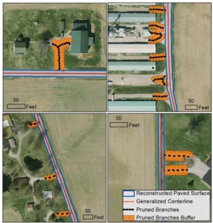
boundary pixel to the centerline; and after that estimating an average road width for each centerline segment of 50 ft intervals for piecewise reconstruction of the paved surface. As mentioned previously, mathematical morphology provides algorithms for the purpose of boundary extraction. We extracted the boundary of the paved surface using morphological operations. This boundary raster still includes the irrelevant branches since the branches have only been removed over the medial axis previously. We removed these branches by masking the boundary raster with large enough buffers generated around branch lines. Next, we generated a boundary distance raster in which each boundary pixel holds its distance to the centerline. The average distance to this boundary is then assigned to the corresponding centerline segment. This allows for the reconstruction of the paved surface extent based on the average width of each centerline segment. Figure 4 shows examples of reconstructed paved surface with branches removed.
Figure 4.Examples of reconstructed paved surface and excluded branches
4.3. Extraction of Cross-section Information
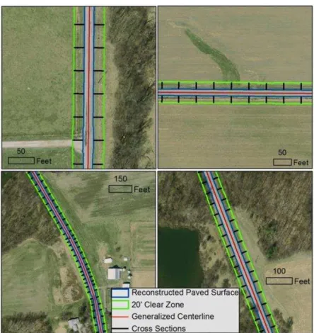
Reconstruction of the paved surface extent provided the means to define the clear zones based on this extent. We established the clear zones around the reconstructed paved surface. Then, we generated cross-section lines corresponding to the center of each centerline segment starting from the extent of the reconstructed paved surface to the extent of the clear zones. Using the DEM, we were able to calculate the slopes along these cross-section lines. Figure 5 shows samples from the cross-section lines from which the side slopes were calculated.
4.4. Extraction of Buildings and Trees
Figure 5.Samples from the 20 ft clear zone and the cross sections along the roads
4.4.1.Ground Filtering
Ground filtering, taken as the initial step before labeling surface and non-surface points significantly reduced the number of points for which the point feature histograms would be calculated. Number of points was reduced from 2,029,115 points to 238,923 points, approximately to 12% of the dataset for this particular study area. We employed the LAStools (Isenburg et. al., 2006) implementation of the iterative TIN densification method of Axelsson (2000) for filtering the ground points.
Calculated point density in the study area is 1.08 pts/m2. We determined the spherical neighborhood radius as 12 ft based on this calculated point density. We applied k-d tree partitioning for the neighborhood range search of off-ground points. Occasionally there were either individual points or small groups of points which were not part of any surface or object. We regarded such points as noise and removed them by applying a threshold for the minimum number of points in their neighborhood.
4.4.2.Local Descriptive Features and Graph Cut Optimization (GCO)
The next step for identifying the objects within the clear zones along the roads was to differentiate between the points that lay on a planar or curved surface and the points that are part of an object which constitutes a 3D manifold. The latter requires the points that are sampled inside the 3D objects instead of just their surfaces. Objects with such sampling are usually the trees and other vegetation since the laser pulse penetrates through the branches and reflections from within the crown are acquired by the LiDAR sensor. Objects that we will refer to as surfaces are usually the planar and curved surfaces of man-made structures excluding the ground since we are only dealing with off-ground points at this stage.
Similar to the work in Ural and Shan (2012), we implemented a min-cut based optimization framework (Boykov et. al., 2001) for labeling 3D off-ground LiDAR points as buildings and
trees, this time using point feature histograms instead of feature vectors. We labeled points by GCO (graph-cut optimization) after calculating the point feature histograms (PFH) for each point.
Point features calculated for each neighborhood represent geometric properties of the neighborhood. Classification of the points with GCO as proposed requires the calculation of the total energy for each labeling, which consists of a smoothness term and data term as
,
,
,
i j i j
i j smooth
E
f
V
f f
(1)
data i
i
E
f
D f
(2)where Vij is the smoothness prior, fi, fj the feature vectors at
sites i, and j, and D the data cost. The data term may be described as a cost value based on the proximity measure between the PFH of the point to be classified and the PFH representing each class. We used the Jeffreys-Matusita (JM) distance in this study. Point features, for which the histograms are to be calculated, are the structure tensor planarity (S.T.P.) and structure tensor sphericity (S.T.S.) features (West et. al., 2004) given as
2 3
1. . .
/
S T P
(3). . .
1
. . .
S T S
S T P
(4)where λ1 > λ2 > λ3 > 0 are the eigenvalues of the covariance
matrix of the point’s local neighborhood.
While the data term of the energy function is calculated in the feature domain, the smoothness term of the energy function is subject to the spatial domain as well as the feature domain. It determines how much a specific labeling of two connected sites needs to be penalized based on the similarity of their features as well as their spatial proximity. It is adjusted by the smoothness parameter σ. The smoothness function
2( , )
(- )
2 ,
1 ,
( , )
f d p q
i j i j
V f f e
d p q
(5)
penalizes the discontinuity between two neighboring sites. The Euclidean distance between points p and q in the spatial domain is d(p,q), and df(p,q) is the feature histogram distance in the
spectral domain. Figure 6 visualizes a sample of calculated data costs for off-ground points for part of the study area.
Once the energy terms are calculated, the remaining task is to find the labeling configuration with the minimum energy. We employed the fast approximate energy minimization algorithm proposed in (Boykov et. al., 2001) via graph cuts over the graph that we established for the point cloud. We set the smoothness parameter σ as 0.8 and α parameter as 1 which defines the relative importance of the data cost.
Figure 6. Examples of data costs of off-ground points calculated for the building (top) and tree (bottom) classes
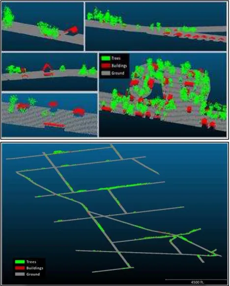
Figure 7. GCO classification results for ground, building and tree classes in parts of the study area (top), and the whole study
area (bottom)
4.4.3.Building Delineation
Ideally, the information regarding detected buildings and vegetation is to be attributable to relevant road segments via spatial queries for the purposes of this study. Dealing with large amount of unstructured points is not an efficient way of storing and querying such information in an operational geographic information database. Hence, a more suitable representation of the extracted information is required. In order to delineate individual buildings, one needs to first determine the points that belong to the same building. It is possible to identify points that belong to individual buildings via connected component analysis. We labeled the points of individual buildings via connected component analysis using octree partitioning.
After the groups of points from individual buildings were segmented by connected component analysis, we delineated the building outlines using α-shape algorithm (Edelsbrunner et. al., 1983). “α-shape” is a generalization of the convex hull of a finite set of points in the plane. We used Pateiro-Lopez and Rodriguez-Casal’s (2010) R implementation of the α-shape algorithm.
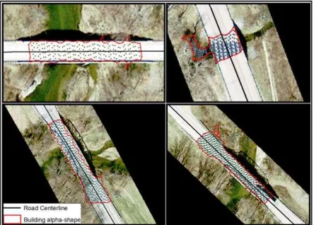
Figure 8. Examples of delineated buildings using the α-shape algorithm
Once the classification results were delineated, we performed the second step filtering for low points which were not to be considered as buildings. Figure 8 shows samples of delineated buildings from parts of the study area. We evaluated building detection results by comparing the classification results with manually digitized building outlines from orthophotos. A total of 140 buildings were delineated from the points classified as buildings. Among these, 43 were false positives including 36 of them being parts of vegetation and seven being either bridges or parts of the roads. 97 buildings out of 107 ground truth buildings were correctly identified. Among these true positives, some building outlines had parts missing since some points that were actually part of the building roofs were classified as vegetation. This happened due to the trees that are too close to the roofs. When compared with the area of the ground truths, seven buildings had more than 50% of their total area missing, while four buildings lost between 30-50% of their total areas and nine of them less than 30%. Table 2 provides a summary of the building detection results and error rates showing false negative (FN), true positive (TP), false positive (FP), false discovery rate (FDR), and false negative rate (FNR) values.
FN TP FP FDR FNR
10 97 43 0.31 0.09
Table 2. Building detection rates
using the medial axis of the road which we extracted from the orthophotos as contextual enforcement. Two of them were not detected since they coincided with the parts of the road which were not successfully reconstructed from the orthophotos due to vegetation cover. Figure 9 shows examples of bridges that were classified as buildings.
Figure 9. Examples of bridges that were classified as buildings, removed from classification results by contextual information.
5. EVALUATION AND CONCLUSION
Despite abundant research efforts, practical and operational capabilities for automated road as well as roadside feature extraction are very limited. We have proposed and implemented a framework for the reconstruction of the road horizontal alignment, the longitudinal grades, the roadway lateral dimensions and the cross slopes, and the roadside areas with obstructions within the identified clear zones. Our contribution considers the extraction of these features relating to road geometry as well as roadside obstructions as an integral and necessary input for a possible road project evaluation system. It is one step forward towards real life transportation planning, construction and operation.
Substantially, we were able to extract 21.3 miles of the road network out of a total length of 23.6 miles in the study area. The nearly 10% difference was due to the portion of the paved surface misclassified and other components removed during the cleaning, simplification and generalization process. Existing road network is not included in any further processing in our framework other than directing to the areas of concern. In case the existing road network is not reliable enough to approximately cover the road surface within a buffer, one would need to perform the road classification task for the entire area covered by the image.
Based on the identified road centerlines, travelled way cross-sections, and roadside areas, we were able to estimate the average grade, identify the cross-section lines, and estimate the cross slopes along these lines at the required longitudinal spacing. Even though we have not encountered steep slopes in the study area, such a situation may happen depending on the topography and the road design. In that case, the resolution of the DEM may limit the accuracy of the calculated slope.
We could extract the obstructions including buildings and trees within a proximity to the road – the important information when evaluating road safety. However, it was not possible to extract vertical features such as fences, walls, posts, signs, etc. due to the limitations of the LiDAR data collected in the study
area. In order to extract such features, mobile, terrestrial, or to some extent, very low altitude airborne LiDAR acquisition would be more suitable. Also, we did not extract individual trees out of a group of trees that are close to each other. Individual trees may be acquired by further processing the points classified as trees. LiDAR dataset with higher point density would be helpful for this purpose.
False positives occurred in two cases of classifying the LiDAR point clouds as buildings or trees. The first group of false positives happened due to the bridges or the road segments with steep side slopes. Such components of roads may be classified as buildings due to their similarity, i.e. high planar surface with respect to the local ground elevation. The second group occurred when the points on the upper parts of the trees formed a planar area similar to the building roofs. This may be filtered out using the NDVI generated from the CIR orthopotos since the spectral response from the trees is different than the response from the buildings.
One challenge in the urban areas was the irregular shape of the roads due to many access points from parking lots, driveways, ramps, etc. We were able to deal with most irregularities via morphological pruning, cleaning, and generalization. We believe that having 90% of the roads extracted together with complementary information as described in mostly suburban and countryside settings provides a feasible semi-automatic data input for practical road project evaluation. It is evident that an additional effort is required to achieve similar results in a dense urban area.
ACKNOWLEDGEMENT
This work was partially supported by the Indiana Department of Transportation, USA.
REFERENCES
Amini, J., Saradjian, M. ., Blais, J. A. ., Lucas, C., and Azizi, A., 2002. Automatic road-side extraction from large scale imagemaps. Int. J. Appl. Earth Obs., 4(2), pp. 95–107.
Axelsson, P., 2000. DEM generation from laser scanner data using adaptive TIN models. In: The International Archives of Photogrammetry and Remote Sensing, Vol. XXXIII, pp. 110-117.
Bacher, U., and Mayer, H., 2005. Automatic road extraction from multispectral high resolution satellite images. In: Proceedings of CMRT05, Vol. XXXVI (3/W24), pp. 29–34. Baumgartner, A., Hinz, S., and Wiedemann, C., 1995. Efficient Methods and Interfaces for Road Tracking. International Archives of Photogrammetry Remote Sensing and Spatial Information Sciences, 34(3-B), pp. 28–31.
Baumgartner, A., Steger, C., Helmut, M., Eckstein, W., and Ebner, H., 1999. Automatic Road Extraction Based on Multi Scale, Grouping, and Context. Photogrammetric Engimeering and Remote Sensing, 65(7), pp. 777–785.
Boyko, A., and Funkhouser, T., 2011. Extracting roads from dense point clouds in large scale urban environment. ISPRS Journal of Photogrammetry and Remote Sensing, 66(6), pp.2– 12.
Boykov, Y., Veksler, O., and Zabih, R., 2001. Fast approximate energy minimization via graph cuts. IEEE Trans. on Pattern Anal. and Mach. Intell., 23(11), pp. 1222–1239.
images. IEEE Trans. Geosci. Remote Sens., 49(10), pp. 3906– 3931.
Dal Poz, A. P., Gallis, R. A B., Da Silva, J. F. C., and Martins, É. F. O., 2012. Object-space road extraction in rural areas using stereoscopic aerial images. IEEE Geosci. Remote Sens. Lett., 9(4), pp. 654–658.
Douglas, D., and Peucker, T., 1973. Algorithms for the reduction of the number of points required to represent a digitized line or its caricature. The Canadian Cartographer, 10(2), pp. 112–122.
Edelsbrunner, H., Kirkpatrick, D., and Seidel, R., 1983. On the shape of a set of points in the plane. IEEE Trans. Inf. Theory, 29(4), pp. 551–559.
French Space Agency (CNES), 2013. Orfeo Toolbox. Available from http://www.orfeo-toolbox.org/otb/about-otb.html
Gamba, P., Dell’Acqua, F., and Lisini, G., 2006. Improving urban road extraction in high-resolution images exploiting directional filtering, perceptual grouping, and simple topological concepts. IEEE Geosci. Remote Sens. Lett., 3(3), pp. 387–391.
Han, J., Kamber, M., and Pei, J., 2012. Data mining: Concepts and techniques. Elsevier. Waltham, MA.
Haralick, R.M., Sternberg, S.R., and Zhuang, X., 1987. Image analysis using mathematical morphology. IEEE Trans. Pattern Anal. Mach. Intell., 9(4), pp. 532-550.
Hedman, K., Hinz, S., and Stilla, U., 2006. A Probabilistic Fusion Strategy Applied to Road Extraction From Multi-Aspect SAR Data. In: International Archives of Photogrammetry, Remote Sensing and Spatial Information Sciences, Vol. XXXVI, pp. 55–60.
Hinz, S., and Baumgartner, A., 2003. Automatic extraction of urban road networks from multi-view aerial imagery. ISPRS Journal of Photogrammetry and Remote Sensing, 58, pp. 83– 98.
Hu, X., Li, Y., Shan, J., Zhang, J., and Zhang, Y., 2014. Road centerline extraction in complex urban scenes from LiDAR data based on multiple features. IEEE Trans. Geosci. Remote Sens., 52(11), pp. 7448–7456.
Isenburg, M., Liu, Y., Shewchuk, J., Snoeyink, J., Thirion, T., 2006. Generating Raster DEM from Mass Points via TIN Streaming. GIScience'06 Conference Proceedings, pp. 186-198. Kumar, P., McElhinney, C. P., Lewis, P., and McCarthy, T., 2013. An automated algorithm for extracting road edges from terrestrial mobile LiDAR data. ISPRS Journal of Photogrammetry and Remote Sensing, 85, pp. 44–55.
Lacroix, V., and Acheroy, M., 1998. Feature extraction using the constrained gradient. ISPRS Journal of Photogrammetry and Remote Sensing, 53, pp. 85–94.
Lam, L., Lee, S., and Suen, C., 1992. Thinning methodologies: A comprehensive survey. IEEE Transactions on Pattern Analysis and Machine Intelligence, 14(9), pp. 869-885. Laptev, I., Mayer, H., Lindeberg, T., Eckstein, W., Steger, C., and Baumgartner, A., 2000. Automatic extraction of roads from aerial images based on scale space and snakes. Machine Vision and Applications, 12, pp. 23–31.
Mayer, H., Laptev, I., Baumgartner, A., and Steger, C., 1997. Automatic road extraction based on multi-scale modeling, context, and snakes. In: International Archives of Photogrammetry and Remote Sensing, Vol. 32, pp. 106–113. Mayer, H., Hinz, S., Bacher, U., and Baltsavias, E., 2006. A test of automatic road extraction approaches. In: The International Archives of Photogrammetry, Remote Sensing and Spatial Information Sciences, Vol. XXXVI, pp. 209–2014.
Mena, J. B., 2003. State of the art on automatic road extraction for GIS update: A novel classification. Pattern Recognition Letters, 24, pp. 3037–3058.
Miao, Z., Shi, W., Zhang, H., and Wang, X., 2013. Road centerline extraction from high-resolution imagery based on shape features and multivariate adaptive regression splines. IEEE Geosci. Remote Sens. Lett., 10(3), pp. 583–587.
Mohammadzadeh, A., Tavakoli, A., and Zoej, M. J. V., 2006. Road extraction based on fuzzy logic pan-sharpened IKONOS images. The Photogrammetric Record, 21(3), pp. 44–60. Naouai, M., Hamouda, A., and Weber, C., 2010. Urban road extraction from high-resolution optical satellite images. In International Conference on Image Analysis and Recognition pp. 420–433. alphahull. Journal of Statistical Software, 34(5).
Poullis, C., and You, S., 2010. Delineation and geometric modeling of road networks. ISPRS Journal of Photogrammetry and Remote Sensing, 65(2), pp. 165–181.
Quackenbush, L. J., 2004. A Review of techniques for extracting linear features from imagery. Photogrammetric Engineering and Remote Sensing, 70(12), pp. 1383–1392. Shi, W., Miao, Z., and Debayle, J., 2014. An integrated method for urban main-road centerline extraction from optical remotely sensed imagery. IEEE Trans. Geosci. Remote Sen., 52(6), 3359–3372.
Soille, P., 1999. Morphological image analysis: Principles and applications. Heidelberg: Springer-Verlag, Berlin.
Soille, P., and Pesaresi, M., 2002. Advances in mathematical morphology applied to geoscience and remote sensing. IEEE Trans. Geosci. Remote Sens., 40(9), pp. 2042–2055.
Steger, C., 1998. An unbiased detector of curvilinear structures. IEEE Trans. Patt. Anal. Mach. Intell., 20(2), pp. 113–125. Theodoridis S., and Koutroumbas, K., (2009). Pattern Recognition. Academic Press, Boston.
Ural, S., and Shan, J., 2012. Min-cut based segmentation of airborne lidar point clouds. In: International Archives of Photogrammetry, Remote Sensing and Spatial Information Sciences. Vol. XXXIX, Part B3, pp. 167-172.
Valero, S., Chanussot, J., Benediktsson, J. a., Talbot, H., and Waske, B., 2010. Advanced directional mathematical morphology for the detection of the road network in very high resolution remote sensing images. Pattern Recognition Letters, 31(10), pp. 1120–1127.
West, K.F., Webb, B.N., Lersch, J.R., Pothier, S., Triscari, J.M., and Iverson, A.E., 2004. Context-driven automated target detection in 3D data. In: Proc. SPIE 5426, Automatic Target Recognition XIV, pp. 133-143.
Yang, B., Fang, L., and Li, J., 2013. Semi-automated extraction and delineation of 3D roads of street scene from mobile laser scanning point clouds. ISPRS Journal of Photogrammetry and Remote Sensing, 79, pp. 80–93.
Zhang, C., 2004. Towards an operational system for automated updating of road databases by integration of imagery and geodata. ISPRS Journal of Photogrammetry and Remote Sensing, 58, pp. 166–186.