MODELLING THE CARBON STOCKS ESTIMATION OF THE TROPICAL LOWLAND
DIPTEROCARP FOREST USING LIDAR AND REMOTELY SENSED DATA
N.A.M.Zaki ab, Z.A.Latif b*, M.N.Suratman c & M.Z.Zainal d
a Centre of Studies for Surveying Science and Geomatics, Faculty of Architecture Planning and Surveying, Universiti Teknologi MARA (UiTM), Shah Alam, Malaysia - [email protected]
b Applied Remote Sensing & Geospatial Research Group (ARSG), Green Technology & Sustainable Development (GTSD) Community Research, Universiti Teknologi MARA (UiTM),Shah Alam, Malaysia -
c Centre for Biodiversity & Sustainable Development, University Teknologi MARA (UiTM), Shah Alam, Malaysia d Centre of Studies for Surveying Science and Geomatics, Faculty of Architecture Planning and Surveying, Universiti Teknologi
MARA, Arau, Perlis. Commission VI, WG VI/4
KEY WORDS: Tropical Rain Forest; Crown Biomass; LiDAR; Aboveground Biomass; Carbon stocks.
ABSTRACT:
Tropical forest embraces a large stock of carbon in the global carbon cycle and contributes to the enormous amount of above and below ground biomass. The carbon kept in the aboveground living biomass of trees is typically the largest pool and the most directly impacted by the anthropogenic factor such as deforestation and forest degradation. However, fewer studies had been proposed to model the carbon for tropical rain forest and the quantification still remain uncertainties. A multiple linear re gression (MLR) is one of the methods to define the relationship between the field inventory measurements and the statistical extracted from the remotely sensed data which is LiDAR and WorldView-3 imagery (WV-3). This paper highlight the model development from fusion of multispectral WV-3 with the LIDAR metrics to model the carbon estimation of the tropical lowland Dipterocarp forest of the study area. The result shown the over segmentation and under segmentation value for this output is 0.19 and 0.11 respecti vely, thus D-value for the classification is 0.19 which is 81%. Overall, this study produce a significant correlation coefficient (r) between Crown projection area (CPA) and Carbon stocks (CS); height from LiDAR (H_LDR) and Carbon stocks (CS); and Crown projection area (CPA) and height from LiDAR (H_LDR) were shown 0.671, 0.709 and 0.549 respectively. The CPA of the segmentation found to be representative spatially with higher correlation of relationship between diameter at the breast height (DBH) and carbon stocks which is Pearson Correlation p = 0.000 (p < 0.01) with correlation coefficient (r) is 0.909 which shown that there a good relationship between carbon and DBH predictors to improve the inventory estimates of carbon using multiple linear regression method. The study concluded that the integration of WV-3 imagery with the CHM raster based LiDAR were useful in order to quantify the AGB and carbon stocks for a larger sample area of the Lowland Dipterocarp forest.
* Corresponding author
1. INTRODUCTION
1.1 Aboveground Biomass and carbon stocks in relation to Climate Change
Forests are crucial for human life. They provide important resources for medicine, foods, habitat for animal and also play an essential role in carbon sequestration (Abd Latif et al., 2011). In the past few centuries, anthropogenic activities and natural consequences has increased the concentration of carbon dioxide including greenhouse gases (GHG) to the atmosphere (FAO, 2015). In year 1992, the United Nation Framework Convention on Climate Change (UNFCC) formed a framework to decrease the GHG conveyed at the United Nations Conference on Environment and Development (UNCED) held in Rio de Janeiro (UNFCC, 2015). In 2007, the Bali Climate Change Conference under United Nations had adopted Kyoto protocol by setting rightfully binding obligation for reduction of GHG gases emission (UNFCC, 1998). During this conference, an important agreement was reached for the developing countries to initiate actions in reducing emissions from
deforestation and forest degradation (REDD) (Pelletier et al., 2012). It sets a collective global target of reducing GHG emissions by about 5% of the 1990 levels by the first commitment period from 2008 to 2012. An amendment made to the protocol in Doha, Qatar, on 8 December 2012, known as the "Doha Amendment to the Kyoto Protocol", aims to reduce GHG emissions by at least 18% below 1990 levels from 2013 to 2020 during the second commitment period (UNFCC, 2015). In continuation to the persistent efforts to combat global warming and restrain associated global risks, developing a method is increasingly important for monitoring, reporting and verification (MRV) mechanism of Reducing Emissions from Deforestation and Forest Degradation (REDD+).
In South East Asia generally, due to the economic factors, it has been historically proven that a lot of primary forest had been cleared for timber extraction and extensive conversion to oil palm plantation, and rubber plantation (Hansen et al., 2013). It is confirmed in a recent forest cover research that shows the main cause of forest loss in South East Asia is the conversion of the forest to cash crop plantation (Stibig et al., ISPRS Annals of the Photogrammetry, Remote Sensing and Spatial Information Sciences, Volume III-7, 2016
2014). Extensive deforestation and conversion have significant impacts from local to regional scales on wide ranges of ecosystem offered by forest such as hydrological and habitat provision (Blackburn et al., 2014). Consequently, many habitats of plants and animal are lost and it impacts the biodiversity and the richness of species contained in the forests.
1.2 Aboveground Biomass for tropical rain forest.
Estimating the aboveground biomass of the forest, and investigating the carbon stock for the tropical rainforest are not easy tasks due to the complex architecture of trees and plants that vary in sizes (Mohd Zaki et al., 2015; Mohd Zaki & Latif, 2016). In order to predict the tree structure parameter using integration of field data and remote sensing technology, models are normally developed by previous researchers (Babcock et al., 2015; Gonzalez et al., 2010; Li et al., 2015; Saeidi et al., 2014). With the present complex structure of tropical forest, there is an enormous uncertainty for carbon stocks estimation. (Figure 1). In order to measure the aboveground biomass and carbon stocks of an area, the fusion of small footprint discrete Light Detection and Ranging (LiDAR) and Very high resolution (VHR) WV-3 (30cm spatial resolution) data had been used to precisely determine the AGB/C stocks for the dominant tree of the study area. Primarily, there are six dominant family species which are Dipterocarpaceae, Euphorbiaceaea, Sapotaceae, Burseraceae, Moraceae, and Lamiaceae. Among them, one of the species is categorized as Critically Endangered (CR) by (IUCN, 2014) which is Hopea Sulcata or Merawan Meranti.
Figure 1. Profile diagram of Tropical rainforest (Turner, 1996)
The model conveyed in this study aims at filling the knowledge gap by assess modelling the carbon stocks of lowland Dipterocarp forest for Malaysia cases. The models for aboveground biomass and carbon stocks needed for forest biomass with the remote sensing environment, and the option that geospatial technology, can be provided in order to support effective forest management. Therefore, the objective of this study includes (i) investigating the relationship between carbon stocks and tree parameter (DBH, tree height, and crown diameter), (ii) developing a model of carbon stocks estimation using Crown Projection Area (CPA) of the emergent and canopy layer of the tree crown and height derived from LIDAR, (iii) producing the map of carbon stocks generated from the model and (iv) predicting the carbon estimation for the broader area of Ayer Hitam Forest Reserve.
2. MATERIAL AND METHODS
2.1 Study Area
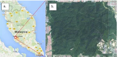
The study area is located at Latitude 3°00'24.19"N, Longitude 101°38'25.24"E in the Ayer Hitam Forest Reserve (AHFR), Selangor State, Malaysia (Figure 2). The data collected from this lowland Dipterocarp forest of Ayer Hitam Forest Reserve chosen for field sampling are owned by University Putra Malaysia (UPM) under custodian of Faculty of Forestry. This secondary forest comprises of various species that are dominant by family tree of Dipterocarpacaea. The altitude that comprises in this lowland forest varies from 15 m to 233 m height, and the terrain slope undulating up to 34º (Shida et al., 2014).The average annual rainfall is 2178 mm while the average temperature annually is 25.3ºC with maximum 27.7º C and minimum 22.9º C (Shida et al., 2014).
Figure 2. A map of the location of the study area. Figure 2a. Shows the location of Selangor District, at Peninsular Malaysia. Fig. 2b shows a location of Ayer Hitam Forest Reserve Lowland Dipterocarp forest covered by the WV-3 satellite image data.
2.2 Airborne Laser Scanning (ALS) Data and WV-3 data
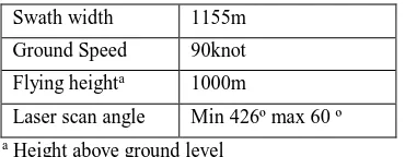
The ALS survey had been flown using a Eurocopter 120 on August 2013. The LiteMapper-Q560 that consist of RIEGL LMS-Q560 laser scanner for LiDAR scanner was mounted on the aircraft, along with the Hassleblad digital camera 39 megapixel with 50mm focal length. Table 1 summarizes the flight parameter used for capturing LiDAR to achieve point density of 11.98 per square units. The projection used is WGS1984 UTM Zone 47N. The ALS survey of raw files was pre-processed using AeroOffice IGI to analyse the quality of IMU and GPS data. Terrasolid tools were used to process the ALS dataset (Bentley Systems, 2015) into LIDAR 3D point clouds. Super-spectral high resolution of WV-3 (8 bands) 25 km2 with the projection of UTM47 N and WGS84 datum, have been used in this study. The data was obtained on 9th December 2014 that consists of 31cm panchromatic band, 4 bands VNIR colours (blue, green, red and NIR-1) and 4 added VNIR colours which are coastal, yellow, red edge and near-IR2. The spatial resolution was 0.30 m (panchromatic) and 1.2 m (multispectral). The classification was performed on a pan-sharpen WV-3 image using hyperspherical colour pan-sharpening (HCS) techniques for better visualization.
System LiteMapper-Q560
Scan angle 45 º
Pulse frequency 150kHz
Overlap Side overlap 40,frontal overlap 60
Swath width 1155m
Ground Speed 90knot
Flying heighta 1000m
Laser scan angle Min 426º max 60 º
a Height above ground level
Table 1. Summary of discrete LiDAR returns and details
2.3 Field sampling plot
Field sampling had been collected using stratification number of sampling, estimated using equation (1). Tree stand sampling and forest mensuration data was collected on May 2015 at 2 ha rectangular that consists 50 subplots included tree id, species, tree ages, stem diameter at breast height (1.3) for live trees which have 10 cm and above, sample of tree height (living tree), crown base height (the height for 1st branches up to the crown), leaf area index and also crown diameter of the canopies.
(1)
Nplot = Minimum number of sampling plots t2 = Value of tree distribution of N
plot CV = Coefficient of Variance (%) E = Allowable error
Field plot and tree coordinates were located by traversing using total station to the plot edge coordinate. Each of coordinate were tied by Global Positioning System (GPS) observation of Topcon GTS using static observation L1/L2 and L5 bands. The positional accuracy of the plot coordinates was generally within ± 0.5 m of the acceptable tolerance. Single tree locations that consist of coordinate, bearing and slope distance were measured for each individual tree in relation with the centre plots for the future use. In all plots, the tree height of forest stands were measured using digital DISTO D5 laser ranger while the DBH (1.3 m above ground height) was measured using a DBH tape.
2.4 Data Preparation and Analysis
Figure 3. Methodology workflow
This study was performed according to three major phases. This comprises of the data collection of the forest stands, data acquisition, pre-processing of the data, object based image analysis (OBIA), model development, validation of the data and finally the statistical analysis. Figure 3 illustrate the process involved in this study.
2.4.1 Canopy Height Model generation: Canopy height model is commonly calculated in the form of raster representation, generate from the highest echo of first return laser pulse known that create the digital surface model (DSM) subtract with the lowest echo of last return which is known as digital terrain model (DTM) (Popescu et al., 2003). Normalization is applied to the CHM which gives the absolute point of height of tree height on Z-axis, and according to the dataset, the maximum tree was 44m. Thus, we drop all the LiDAR points that are higher than the value of maximum tree, as a noise. The CHM was created using LAStools software in ArcGIS plug-in. Figure 4 show the CHM of the tree height in 3Dimension (3D) view.
Figure 4. Canopy height model. Figure 4a. The top view of the CHM of the study area. Fig. 4b. The 3D view from the top of CHM, Fig. 4c. The interpolation of height of the CHM and finally Fig. 4d. The perspective view of the CHM of the study area.
2.4.2 Estimation Carbon stocks using allometric equation: AGB estimation were calculated using allometric equations (Chave et al., 2014) (Equation 2) that uses wood density, height and DBH as predictors. Wood density is an important predictor in the calculation of AGB based on species despite of the height and DBH (Fayolle et al., 2013). The details of each tree were recorded as: total height ht, bole height hb, crown diameter ci, diameter at 1.30m height di and species.
….. (2) Where AGB = Aboveground biomass (kg / tree), ρ = wood density, E = Bioclimatic variables and D = diameter at breast height (DBH).
On the basis, carbon were converted by applying the conversion factor of 0.47 which represents 47% of the dry biomass assumed to be carbon for all part of the tree as the default value that had been recommend by IPCC (IPCC, 2006).
2.4.3 Crown Projection Area (CPA) delineation and validation: There are many approaches in calculating the accuracy assessment of segmentation based on literature but the most common method used is by visual (Mohd Zaki et al., 2015)Previous researchers have used different type of segmentation validation by overlapping the area that intersect between output segmented area with reference area (Möller et al., 2007). Another researcher used the distance between two centroids to assess the segmentation accuracy (Ke, Quackenbush, & Im, 2010). On the other hand , Gougeon (1995) had developed the segmentation validation using 1:1 spatial corresponding based on goodness of fit (D). However, Clinton et al., (2010) had improve the segmentation validation method developed by Ke et al., (2010) and Möller et al., (2007) by modifying the relative area metrics by calculating Equation (3) and (4) and measuring the goodness of fit by using Equation (5).
……… (3)
………... (4)
…... (5)
Segmentation accuracy is measured based on distance index (D) ranging from 0 to 1, where 0 shows that the classification is an ideal match between xi and yi, while 1 is the minimum mismatch. In order to evaluate the multi-resolution segmentation, this study has applied evaluation approach by Clinton et al., (2010) where it measures the segmentation goodness measures.
2.4.4 Statistical analysis: The correlation between CS stocks, height, DBH and CPA were analysed using Pearson’s correlation as well as multiple linear regression model. Bootstrap sampling was executed in order to account for the small value of tree stands. The statistical analysis is proceeded by performed by calculating statistical parameter such as residual R2, adjusted R2, Root Mean Square Error (RMSE) (Equation 7), segmentation validation and height validation. The multi-collinearity test also had been done in order to avoid any collinearity problem between variables, with a tolerance cut of value of variance inflation factor (VIF) should be less than 10 (O’Brien et al., 2007) (Equation 6).
….. (6)
Where is the squared multiple correlation of the variables of jth explanatory variable in the regression model (Equation 6). During the classification of the segmentation of the individual tree, one to one matching of reference and segmentation tree crowns was used for developing the model. Then, the model were validated with 30% of field sampling data out of 911 number of tree stands that had been measured.
…….. (7)
Where n is the number of samples, yi is the calculated value of carbon, is the predicted carbon by model of the response variables.
3. ANALYSIS AND DISCUSSION
The analysis of this research comprises of the description of studies, normality, and correlation analysis. The following paragraphs will explain the results of these analyses.
3.1 Descriptive statistics
Overall, the amount of tree sampling of the whole study area at Ayer Hitam Forest Reserve was 911 trees collected from 50 subplots within 2 ha plots. The accuracy of GPS observation at the base station was 3 mm for horizontal (x and y) and 5mm for vertical (z) plot. In total, 911 of tree had been measured from the observation where six dominant genuses had been identified: Dipterocarpaceae, Euphorbiaceaea, Burseraceae, Sapotaceae, Moraceae, Rhizophoraceae and Rubiaceae. Dominant species nominated by Endospermun diadenum, Hopea Sulcata, Shorea Macroptera and Dipterocarpus Verucosus. In order to ensure representative, 183 of tree were randomly selected in each subplot, while the other 62 trees (30%) were used as a reference (Figure 5).
Figure 5. Box plot of data collection from field data (DBH, height, crown diameter and bole height). Fig. 5a. Show the boxplot of DBH of the tree stands, Fig. 5b. The height of the tree, Fig. 5c. The crown diameter of the tree stands and Fig. 4d. The bole height which is the height from of the first branch.
3.2 Normality test for model development
The selection predictor variables had analysed the normality test used for the model development. The resultrepresents the distribution of DBH, height from field, height from LiDAR and
a.) b.)
c.) d.)
crown projection area derived from the fusion of LiDAR and multispectral WV-3.
Kolmogorov-Smirnova Shapiro-Wilk Statistic df Sig. Statistic df Sig. DBH 0.048 183 0.200 0.984 183 0.041 H_Fiel
d
0.073 183 0.018 0.983 183 0.026
H_LD R
0.053 183 0.200 0.985 183 0.052
CPA 0.058 183 0.200 0.984 183 0.038 *.This is a lower bound of true significance
a. Liliefors Significance Correction
Table 2. Normality test for model development.
Based on the finding, this shows the output of the Kolmogorov-Smirnov and the ShapiroWilk tests for the distribution of DBH, height (field), height (LiDAR), and CPA. For both test, p-value was nearly normal distributed (P > 0.01) (Table 2). The log transformation had been applied to make sure that the data is normally distributed for the all dependent variables thus to make a perfectly linear regression (Piaw, 2014).
3.3 Validation of LiDAR derived height
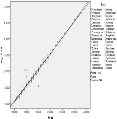
With regards to the analysis, the highest positive r value was recorded for height LiDAR versus height field which is 0.995 (Figure 6) which shows that there is a strong correlation between height LiDAR and height field. Besides, there is no significant difference (p > 0.01) between height measured from field and height derived from LiDAR. However, there is a strong correlation between height measured from field and height derived from LiDAR. Table 3 and Table 4 summarize the output result of the compare means between heights LiDAR versus height field of 245 sample of tree.
Figure 6. The relationship between tree height from field (Ht_m) and tree height derived from LiDAR (Ht_LIDAR).
Table 3. Summary of statistical –Tree height from field and LiDAR data
Correlation of coefficient 0.991
R2 Linear 0.982
Adjusted R2 0.982
Standard Error 0.699
RMSE 0.486
Intercept 0.739
Number of sample 245
Table 4. Overall summary of fit
3.4 Accuracy assessment of segmentation output
Accuracy assessment of the tree crown segmentation had been applied in two techniques, which is i.) By using techniques 1:1 matching of the references and segmentation polygon, ii.) Quantify the goodness of fit (D) which represents the ideal segmentation. Based on Table 5, it is shown that the average accuracy of the segmentation is 79.5%. Out of 288 manually delineated of the crown, only 266 were matched 1:1 (78% match). The over segmentation and under segmentation value for this output is 0.19 and 0.11 respectively ,thus D-value for the classification is 0.19 which is 81% .The result shows that the segmentation output are acceptable for further analysis. (Figure 7).
Table Head
Accuracy Segmentation Total
Reference Polygon
Total 1:1 match
OS US D
1:1 288 266
Goodness of fit
0.19 0.11 0.19
Total accuracy
78% 81%
(OS = over segmentation, US = under segmentation and D = Goodness of fit)
Table 5. Accuracy assessment of OBIA output
Figure 7. The segmented (Red colour) and Reference (Yellow) polygon
Test F P value t df
Pearson’s correlation
12963.067 0.052 -1.950 244
T-Test 0.011 0.918 -1.041 488
3.5 Correlation analysis –Pearson correlation
In an effort to see the relationship between these variables, for example, between DBH and height LiDAR, height field and CPA, Pearson correlation had been done to measure the correlation between independent variables of carbon estimation. **Correlation is significant at the 0.01 level (2-tailed)
(PC= Pearson Correlation, N = number of samples, H_LDR = tree height from LiDAR, H_Field = tree height from field, CPA = crown projection area, .Sig = significant level)
Table 6. Pearson correlation of the DBH, H_LDR and CPA.
From the analysis, the highest positive r value was recorded for H_LDR versus H_Field which is 0.995 which shows that there is a strong correlation between height LiDAR and height field (P < 0.01). As a result, there is strong evidence that suggests that this correlation is significant. The positive correlation between Ht_LiDAR and DBH showed in Table 6, which depicted that the high correlation between this two variables (0.763) with (P < 0.01). The results show that there is a high correlation between height LiDAR and DBH.
Pearson correlation analysis of the independent variables is used to calculate the carbon stocks where carbon as the dependent variable. High positive relationship between DBH and carbon stocks was found with (P < 0.01) (Table 6). The data yielded by this study provides strong evidence. Multiple regression model was developed using LiDAR derived height and CPA as independent variable and carbon as a dependent predictors. (See Table 7, Table 8 and Table 9).
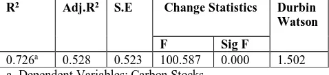
a. Dependent Variables: Carbon Stocks b. Predictors: (Constant), H_LDR and CPA
Table 7. Model summary
Regression 17245373. 2 8622686. 10 0
0.00b
Residual 15430193. 180 85723.2
Total 32675567. 182
a. Dependent Variables: Carbon Stocks b. Predictors: (Constant), Ht_LiDAR and CPA
Table 8. ANOVAa 3.6 The multiple linear regression analysis
Based on the regression, there was a negative linear relationship between predictor and output variables, β = -2971.429, ρ = 0.000 (p < 0.01). Multi-collinearity between the two variables had been checked by applying the variance inflation factor (VIF) test where the result shows that there was no sign of multi-collinearity found between these two variables (VIF= 1.363). By using multiple regression model to predict the carbon stocks estimation over the height derived from LiDAR and crown projection area was a negative predictors, β = -2971.429, p = 0.000 (p < 0.01) disputed that every unit increase of carbon stocks, the height from LiDAR and CPA were decreased by -2971.429m. Thus, the relationship of carbon stocks can be written as the following equations:
… (7)
...(8)
The coefficient demonstrated in Table 9 represents the effect size, beta = 0.726. Moreover, the result shows that the Durbin-Watson value is 1.502 which exemplifies that autocorrelation is within the tolerance where the Analysis of variance (ANOVA) test indicates that the overall model are significant, p = 0.000 (p < 0.01).
3.7 Validation of multiple linear regression model
Pearson’s product- model of tree crown was validated using a random selection of 30% of the independent dataset which is in this case 62 trees from various types of tree height and species. The resulting coefficient of determination between carbon predicted and the carbon observed was 0.6737 (R2 = 0.6737)
Figure 8. Scatter plot of multiple regression model validation
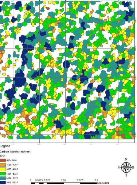
3.8 Carbon Stocks Map
In brief, the range of the predicted carbon is around 800 kg/trees to 7634 kg/tree where it can be concluded that the higher the CPA and height value, the greater the amount of carbon it would make. Figure 9 shows that the darker colour of the CPA which indicates the highest value of carbon, while the white colour of the background of the map is the gap of each individual tree. The carbon stocks map of the study area is shown in (Figure 9).
Figure 9. Carbon stocks of the study area
(Karna (2013) found out that a significant correlation coefficient (r) between (CPA – Carbon), (height – Carbon), and (CPA – Height) is 0.73, 0.76 and 0.63 respectively. Similar to this relationship, this study produced 0.671, 0.709 and 0.549 for the type of Lowland Dipterocarp forest which mainly focuses on tropical rain forest. However, the highest correlation exemplified by the relationship between DBH and carbon stocks which is Pearson Correlation (0.909) shows that there is a good relationship between carbon and DBH predictors to improve the inventory estimation of carbon using multiple linear regression method.
4. CONCLUSION AND RECOMMENDATION
This paper presents a model development from fusion of CHM derived from LiDAR and WorldView-3 imagery using the MLR-based methodology to estimates the forest biomass from remote sensing technology. The combination of LiDAR and Very High Resolution Multispectral Imagery, WV-3 has demonstrated a promising capability to model the aboveground biomass and carbon stocks needed for forest biomass estimation for lowland Dipterocarp forest. Results indicate that the relationship between carbon stocks with LiDAR and CPA obtained in this study are similar in terms of correlation produce and the levels of variances with other studies that have been done previously (Karna et al., 2013). The output MLR shown that there is non-linear equation of the predicted model where the natural logarithmic had been used and get the better prediction. Future works should address the gaps that did not cover in this paper. The primary limitation of the methods is the robust of the complexity intermingles of the tropical forest itself and the improvement of the CPA delineation should be address. Finally, the synergistic use of the non-parametric test comparing with this traditional regression analysis, MLR will be the future works in order to estimate the biomass and carbon stocks of the tropical rainforest.
ACKNOWLEDGEMENTS
The authors would like to express their deepest gratitude to the Ministry of Higher Education (MOHE), Malaysia for financing the research under Research Acculturation Grant Scheme (Ref:: RAGS/1/2014/STWN10/UITM//1) Universiti Teknologi MARA (UiTM) and also to Faculty of Forestry, Universiti Putra Malaysia (UPM) for granting access to the study area. Thanks to Alhaffiz Abd Radzak (RS GIS Consultancy Sdn Bhd) for LiDAR pre-processing. Special thanks to Ms Mebrat Tikabo (University of Twente, Netherlands) for the advice on statistical interpretation.
REFERENCES
Abd Latif, Z., Aman, S. N. A., & Ghazali, R. (2011). Delineation of tree crown and canopy height using airborne LiDAR and aerial photo. 2011 IEEE 7th International Colloquium on Signal Processing and Its Applications, (2), 354–358.
Babcock, C., Finley, A. O., Bradford, J. B., Kolka, R., Birdsey, R., & Ryan, M. G. (2015). LiDAR based prediction of forest biomass using hierarchical models with spatially varying coefficients. Remote Sensing of Environment, 169, 113–127.
Bentley Systems. (2015). TerraScan User’s Guide. Retrieved from https://www.terrasolid.com/download/tscan.pdf
Blackburn, G. A., Abdul Latif, Z., & Boyd, D. S. (2014). Forest disturbance and regeneration: a mosaic of discrete gap dynamics and open matrix regimes? Journal of Vegetation Science, Volume 25(Issue 6), pages 1341–1354.
Chave, J., Réjou-Méchain, M., Búrquez, A., Chidumayo, E., Colgan, M. S., Delitti, W. B., … Vieilledent, G. (2014). Improved allometric models to estimate the aboveground biomass of tropical trees. Global Change Biology, Volume 20(Issue 10), 3177–3190.
Clinton, N., Holt, A., Scarborough, J., Yan, L., & Gong, P. (2010). Accuracy Assessment Measures for Object-based Image Segmentation Goodness. Photogrammetric Engineering And Remote Sesing, 76(3), 289–299.
FAO. (2015). Global Forest Resources Assessment 2015
(ISBN 978-9.). Retrieved from
http://www.fao.org/forestry/fra2005/en/
Fayolle, A., Doucet, J.-L., Gillet, J.-F., Bourland, N., & Lejeune, P. (2013). Tree allometry in Central Africa: Testing the validity of pantropical multi-species allometric equations for estimating biomass and carbon stocks. Forest Ecology and Management, 305, 29–37.
Gonzalez, P., Asner, G. P., Battles, J. J., Lefsky, M. a., Waring, K. M., & Palace, M. (2010). Forest carbon densities and uncertainties from Lidar, QuickBird, and field measurements in California. Remote Sensing of Environment, 114(7), 1561–1575.
Gougeon, F. (1995). A crown-following approach to the automatic delineation of individual tree crowns in high spatial resolution aerial images. Canadian Journal of Remote Sensing, 21(3), 274–284.
Hansen, M. C., Potapov, P. V, Moore, R., Hancher, M., Turubanova, S. a, Tyukavina, a, … Townshend, J. R. G. (2013). High-resolution global maps of 21st-century forest cover change. Science (New York, N.Y.), 342(6160), 850–3.
IPCC. (2006). Guielines for National Greenhouse Gas Inventories Volume 4 Agriculture,Forestry and other Land Use,
4. Retrieved from
http://www.ipcc-nggip.iges.or.jp/public/2006gl/
IUCN 2014. (2014). The IUCN Red List of Threatened Species. Retrieved from <http://www.iucnredlist.org>.
Karna, Y. K., Hussin, Y. A., Gilani, H., Bronsveld, M. C., Murthy, M., Qamer, F. M., … Bhattarai, T. (2013). Integration of WorldView-2 and airborne LiDAR data for tree species level carbon stock mapping in Khayar Khola watershed, Nepal. ISPRS Journal of Photogrammetry and Remote Sensing, In Review, 280–291.
Ke, Y., Quackenbush, L. J., & Im, J. (2010). Synergistic use of QuickBird multispectral imagery and LIDAR data for object-based forest species classification. Remote Sensing of Environment, 114(6), 1141–1154.
Li, W., Niu, Z., Liang, X., Li, Z., Huang, N., Gao, S., … Muhammad, S. (2015). Geostatistical modeling using LiDAR-derived prior knowledge with SPOT-6 data to estimate temperate forest canopy cover and above-ground biomass via stratified random sampling. International Journal of Applied Earth Observation and Geoinformation, 41, 88–98.
Mohd Zaki, N. A., Abdul Latif, Z., & Zainal, M. Z. (2015). Aboveground Biomass and Carbon Stock Estimation Using Double Sampling Approach and Remotely-Sensed Data. In Environmental and Civil Engineering Technology International Conference 2015 (ENVICET 2015), Krabi, Thailand (Vol. 1, pp. 1–6).
Mohd Zaki, N. A., Abdul Latif, Z., Zainal, M. Z., & Zainuddin, K. (2015). Individual Tree Crown ( ITC ) Delineation Using Watershed Transformation Algorithm For Tropical Lowland Dipterocarp. Proceedings of the IEEE 2015, 2, 237–242.
Mohd Zaki, N. A., & Latif, Z. A. (2016). Carbon Sinks and Tropical Forest Biomass Estimation: A Review on Role of Remote Sensing In Aboveground-Biomass Modelling. Geocarto International, 6049(April), 1–41.
Möller, M., Lymburner, L., & Volk, M. (2007). The comparison index: A tool for assessing the accuracy of image segmentation. International Journal of Applied Earth Observation and Geoinformation, 9, 311–321.
O’Brien, R. M. (2007). A Caution Regarding Rules of Thumb for Variance Inflation Factors. Quality & Quantity, 41(5), 673– 690.
Pelletier, J., Kirby, K. R., & Potvin, C. (2012). Significance of carbon stock uncertainties on emission reductions from deforestation and forest degradation in developing countries. Forest Policy and Economics, 24, 3–11.
Piaw, C. Y. (2014). Basic Research Statistic (Fourth Edi.). Mc Graw Hill.
Popescu, S. C., Wynne, R. H., & Nelson, R. F. (2003). Estimating plot-level tree heights with lidar: Local filtering with a canopy-height based variable window size. Computers and Electronics in Agriculture, 37(1-3), 71–95.
Saeidi, V., Pradhan, B., Idrees, M. O., & Abd Latif, Z. (2014). Fusion of Airborne LiDAR With Multispectral SPOT 5 Image for Enhancement of Feature Extraction Using Dempster-Shafer Theory. Geoscience and Remote Sensing, IEEE Transactions on, PP(99), 1–9.
Shida, N., Hanum, F., W.M, W. R., & K, K. (2014). COMMUNITY STRUCTURE OF TREES IN AYER HITAM FOREST RESERVE , PUCHONG ,. THE MALAYSIAN FORESTER, 77(1), 73–86.
Stibig, H.-J., Achard, F., Carboni, S., Raši, R., & Miettinen, J. (2014). Change in tropical forest cover of Southeast Asia from 1990 to 2010. Biogeosciences, 11(2), 247–258.
Turner, I. M. (1996). The Ecology of Trees in the Tropical Rain Forest. The Journal of Applied Ecology, 33, 1–314. UNFCC. (2015). UNFCC. Retrieved May 20, 2015, from http://unfccc.int/kyoto_protocol/items/2830.php