SATELLITE IMAGERY ASSISTED ROAD-BASED VISUAL NAVIGATION SYSTEM
A. Volkovaa∗, P.W. Gibbensb,
aStudent Member, IEEE, PhD candidate, School of Aerospace, Mechanical and Mechatronic Engineering,
The University of Sydney, Australia - [email protected] b
Associate Professor, School of Aerospace, Mechanical and Mechatronic Engineering, The University of Sydney, Australia - [email protected]
KEY WORDS:Unmanned aerial vehicle (UAV), Navigation, Vision, Accurate road centreline extraction, Feature-based visual navi-gation, Splines
ABSTRACT:
There is a growing demand for unmanned aerial systems as autonomous surveillance, exploration and remote sensing solutions. Among the key concerns for robust operation of these systems is the need to reliably navigate the environment without reliance on global navigation satellite system (GNSS). This is of particular concern in Defence circles, but is also a major safety issue for commercial operations. In these circumstances, the aircraft needs to navigate relying only on information from on-board passive sensors such as digital cameras. An autonomous feature-based visual system presented in this work offers a novel integral approach to the modelling and registration of visual features that responds to the specific needs of the navigation system. It detects visual features from Google Earth†to build a feature database. The same algorithm then detects features in an on-board cameras video stream. On one level this serves to localise the vehicle relative to the environment using Simultaneous Localisation and Mapping (SLAM). On a second level it correlates them with the database to localise the vehicle with respect to the inertial frame.
The performance of the presented visual navigation system was compared using the satellite imagery from different years. Based on comparison results, an analysis of the effects of seasonal, structural and qualitative changes of the imagery source on the performance of the navigation algorithm is presented.
1. INTRODUCTION
Unmanned aerial vehicles (UAVs) are currently seen as an op-timal solution for intelligence, surveillance and reconnaissance (ISR) missions of the next generation. Compared to human-operated flights, UAVs offer more flexibility and allow for higher risk and are generally less expensive. Employed for various tasks from urban planning and management to exploration and map-ping, most unmanned aerial systems have become highly depen-dent on the accuracy of their navigation system. Moreover, on surveillance and investigation missions such vehicles are sub-jected to the risk of losing its primary source of navigation infor-mation, GNSS due to jamming, interference, unreliability, or par-tial or complete failure. Commercial operations in environments such as so-called urban canyons where GNSS may be unreliable or inaccurate due to multi-path or occlusion, robust operation of the navigation system becomes a serious safety issue and other, preferably passive, sensors become necessary for robustness. To allow tolerance to GNSS faults, a UAV needs to be given a capability to maintain its course and continuously localise rely-ing on a backup passive navigation information source like a vi-sual navigation system (VNS). Since the acceptable precision of on-board inertial-based navigation system is limited to relatively short periods of time due to the integration of sensor measure-ments containing errors, a regular update, usually provided by GNSS, is required. With the satellite information being poten-tially unavailable in an uncharacterised environment, a position update can be generated by a VNS coupled with simultaneous lo-calisation and mapping (SLAM). Visual features detected in the image, registered in database can provide an instantaneous posi-tion update that limits the localisaposi-tion uncertainty of the inertial solution to a minimum.
∗Corresponding author
†The algorithm is independent of the source of satellite imagery im-agery and another provider can be used
Aerial imagery contains all the necessary information about the position and motion of the aircraft. Recently, the research com-munity has been focused on developing methods to retrieve this information from imagery by means of feature-based extraction. While methods developed for Micro Aerial Vehicles (MAVs) mostly use Scale-Invariant Feature Transform (SIFT) or Speeded-Up Robust Feature (SURF) [1-3] feature matching algorithms, the algorithms developed primarily for geographic information system (GIS) update show a semantic, or meaningful, approach to feature extraction. Although it has been recently shown that real-time motion tracking based on small image patches can be very precise [4], the use of such features for SLAM and data as-sociation on level flight over repeatable terrain has not been in-vestigated.
suits the requirements of the navigation system.
2. RELATED WORK
The most complete review on the topic of road extraction was pre-sented in Mena [5] and an elaborate comparison of various road extraction methods was conducted by Mayer [6]. A recent sur-vey of the road extraction algorithms satisfying the requirements of visual aerial navigation systems can be found in Volkova [7]. Below, a brief overview of the feature extraction approaches is provided, focusing on algorithms designed for navigational pur-poses.
Research on the visual-aided navigation has been ongoing for more than two decades [8]. Typical road extraction approaches for the update of map and GIS information are designed as pipelines consisting of image segmentation, extraction and connection of road candidates and final network refinement. SVM classifier [9-12], tensor voting feature detector [13-16] and non-maximum suppression for road centreline extraction [16-23] have been pop-ular road network update techniques. Although, these techniques are superior in quality to direct intensity-based classification and mathematical morphology, they are much more computationally demanding.
Recent corner-based and patch-based real-time motion estima-tion approaches [4, 24, 25] for MAVs achieved high robustness in scenes with high-frequency self-similar texture. A UAV Naviga-tion System presented in [27] combined point-based visual odom-etry with edge-based image registration. Since low-level features used in odometry-based algorithms are often not unique and can only be used in conjunction with depth information, they are use-ful in the short-term especially micro and mid-scale platforms but cannot be the sole basis of a SLAM-based visual navigation sys-tems on a larger scale.
Visual navigation using higher level features (houses, roads, etc.) has been the focus of far fewer research works, partially due to a variety of features representing any one class. Such GIS features as lines (roads), points (road intersections) and regions (forests, lakes, buildings) were suggested for use in navigational system [22, 28] with special attention given to intersections [29, 30]. The rest of this section provides an overview of the approaches that, in the authors’ opinion, are most relevant to the current research. Vision systems focused on landmark detection in [19] utilised a combination of SURF-based image registration and road and building detection using Haar classifiers. Haar training involves creation of a large dataset of the buildings regions and road inter-sections. Although the comparison presented in the above work showed that the Haar classifier outperformed line-based intersec-tion detectors and edge-based building detectors under various il-lumination conditions, its inability to deal with rotation increased the complexity of the system. The GIS-based system presented in [22] registered meaningful object-level features such as road centrelines, intersections and villages in real-time aerial imagery with the data of geographic information system (GIS). The road was extracted using Local Weighted Features (LWF), an approach to estimate the background value of a pixel based on local neigh-bourhood pixels. Subsequently, road end points, branch points and cross points were generated from extracted road networks and were matched with a GIS database.
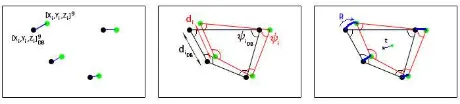
Three-stage landmark detection navigation proposed in [31] ex-tracted a few (3-10) significant objects per image, such as rooves of buildings, parking lots etc., based on pixel intensity level and the number of the pixels in the object. For each of the extracted objects the feature signature was calculated, defined as a sum of the pixel intensity values in radial directions for a sub-image en-closing the feature. The centroids of the extracted objects were simultaneously used to form a waypoint polygon. The angles
between centroids and ratios of polygon sides to its perimeter were then used as scale and rotation-invariant features describing a waypoint in the database.
The autonomous map-aided visual navigation system proposed in this paper combines intensity and frequency-based segmenta-tion, high-level feature extraction and feature pattern matching to achieve reliable feature registration and generate the position and orientation innovations restricting the inertial drift of the on-board navigation system.
3. AUTOMATIC ROAD FEATURE EXTRACTION AND MATCHING (ARFEM) ALGORITHM
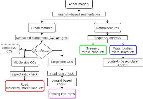
This paper has the goal to provide on-board inertial navigation system with a localisation update calculated from the match be-tween localised visual features registered in an image and a pre-computed database. The proposed multi-pronged architecture of the feature-extraction algorithm is shown on Fig.1. Although the overall structure of the system involves detection of features of greenery and water classes, the specific focus of this paper is on the road-detection component. To generate localisation update, an automatic Road Feature Extraction and Matching algorithm has been developed. The algorithm analyses each image frame to detect the features belonging to one of several classes. It then refines, models, and localises the features and finally matches it to a database built using the same algorithm from Google Earth imagery. In the following section each of these steps of the algo-rithm is detailed.
3.1 Image classification
The first stage of the feature detection algorithm is intensity-based image segmentation. A maximum likelihood classifier trained on 3-5 images for each class was used to detect road, greenery and water regions in the image based on pixel colour, colour variance and frequency response (for the latter two classes). The result-ing class objects were taken through the pipeline shown in Fig.1 to minimise the misclassification and improve the robustness of feature generation. This process is described in detail as the fol-lowing.
The aerial image was classified into road, greenery, water, and background regions using the training data for each class. While road class training was based on intensity of the pixels only (Fig.2), the greenery class description also contains Gabor frequency re-sponse of the provided training region that allows discriminating it from water, which is similar in intensity. At the current stage of algorithm development objects of greenery and water classes
are used for detection of the environment in which the system is operating to adapt the detection techniques accordingly. Future realisation of the system will include processing threads for the corresponding classes and incorporation of localisation informa-tion derived from them.
3.2 Road class filtering
Since reliance on training only in image classification can result in misclassification, further filtering of the classes based on a-priori knowledge about the nature of features in each class is per-formed. The most probable misclassification is between regions of confined water and greenery, and inclusion of road-like ob-jects (parking lots, roofs) into the road components. To extract the road candidates from the urban features category of classes, connected component (CC) analysis [32] was used. The com-ponents were analysed with respect to size and compared with a thresholdAthresh. Components smaller than the threshold were discarded. Middle sized features with high bounding ellipse as-pect ratio [16] were selected. Asas-pect ratio (shown on Fig.3) is calculated as follows.
ARi=
ai
bi
>> tAR, (1)
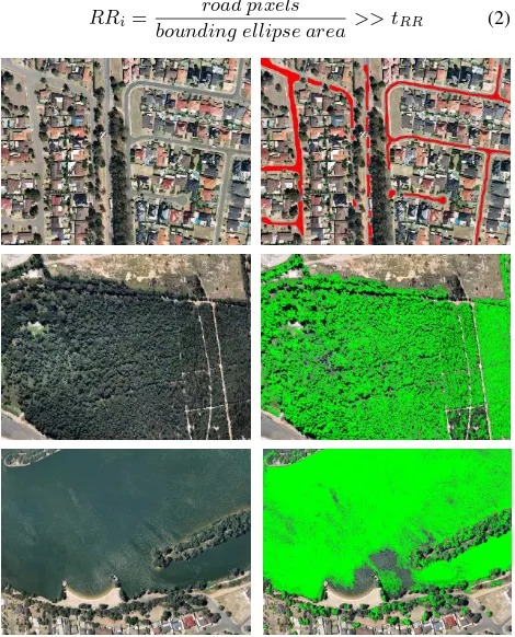
wheretARis an aspect ratio threshold. Aspect ratio [16] elim-inates the misclassification in the road class due to inclusion of rooves and other non-road objects. In cases, where a bounding ellipse is drawn around a curved road segment (Fig.3, centre), the ellipse semi-minor axis is no longer a good approximation to the width of the road. To prevent such components from being discarded, a road ratio check is applied. The road ratioRRiis calculated by estimating the ratio of the road pixels to the total number of pixels within the bounding ellipse:
RRi=
road pixels
bounding ellipse area>> tRR (2)
Figure 2: Training images and ground truth shown for road, greenery and water classes
Figure 3: Comparison of bounding ellipses with bounding box method for straight (left) and curved road components (centre); the area of bounding ellipse in lilac compared to the area of the road component in black(right)
Figure 4: Flowchart of road network generation from road com-ponents detected in the image
For parking lots the road ratio would be considerably larger than the empirically defined thresholdtRR, road segments in turn would have a relatively low RR. The generated road component was processed with trivial morphological operations to improve the robustness of the centreline generation.
Natural features that include water bodies, forests, bush etc. are analysed using frequency analysis. Generally, water areas give higher frequency response, which allows for discrimination be-tween the two. Glare present on the water remains one of the major segmentation problems for intensity-based approaches. Al-though further frequency analysis can be effective in glare detec-tion it is a more computadetec-tionally demanding operadetec-tion compared to contextual solution.
We propose to distinguish between glare and other features sim-ilar in intensity based on the surrounding or neighbouring con-nected components and assign the glare region to the same class. For example, if a glare region is found in the image within the water region but comes up as a road-similar component based on its intensity, it can be filtered from the road class and inserted into the water class (processes marked with * in Fig.1). This glare pro-cessing routing works with the underlying assumption that there are no built-up areas or islands in the confined water regions.
3.3 Road centreline extraction and extrapolation
graph that describes the location and the length of the road seg-ments together with road intersections is obtained. Further anal-ysis and post-processing of road segments and intersections leads to a reliable road network description for further data association.
3.3.1 Extrapolation-based segment joining Some of the road branches in the road graph appear to be incomplete because of the occlusion or the rapid intensity change of the road surface in the image. To address these shortcomings, the following road branch search and connection method is proposed. Splines were fitted to the branch points and then extrapolated in the direction outward from the tip of the branch (Fig.5). The search areas (marked in red) were then checked for the presence of the tips of other branches. In case a tip of another branch is found within the search region, the algorithm suggests joining the branches. If the search initiated from the opposite branch finds the first branch, the branches will be joined.
3.3.2 Road centreline modelling with splines Road branches obtained in the previous stage are heavily influenced by road oc-clusions. For instance, in the presence of the trees along the road side, the road component will decrease in width and therefore its centreline will be shifted to the side opposite to occlusions. To address this problem splines are fitted to model the road in a way in which they capture the most information about the road cen-treline. Similar to the approach to coast line modelling in [33] this work adopts the B-splines fitting described in [34] for road centreline modelling. Here we improve the road modelling by adjusting the locations of the spline nodes to reflect the curvature of the road as follows. First a spline is fitted to road branch pixels to provide filtered coordinates of the branch.
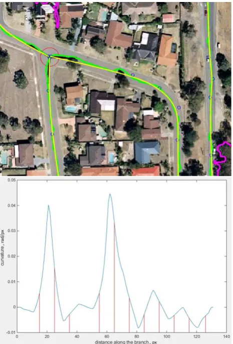
The curvature of the obtained filtered branch is analysed1 by first fitting polygons to the points and then calculating the analyt-ical curvature between consequent points of the polygons. Fig-ure 6 (bottom) illustrates the process of curvatFig-ure accumulation, where the location of the nodes on the branch are marked with red lines. The curvature threshold is set based on scale of the image, with lower threshold for images with lower scale (taken at low altitudes) and higher threshold for images taken from higher alti-tudes, that allows recording of all significant changes in road di-rection and discards the insignificant fluctuations due to the pres-ence of occlusions.
Modelling road branches with splines is an effective method of converting the pixel information into scale independent form, since a spline describes the shape of the feature independent of the scale at which the feature is observed. Splines also minimise
1Matlab function LineCurvature2D by D. Kroon, University of
Twente
Figure 5: Image of extrapolation search (red rectangles) for se-lected road branches (green)
Figure 6: (top) Road branch points generated by thinning (green) are modelled with a spline (yellow); (bottom) curvature of the road branch with locations of the nodes shown in red
the amount of information with which the feature is encoded and therefore are preferable for feature matching and data association.
T- junctions
The skeletonisation operation often causes the offset of the T-junction centroid in the direction of the connecting branch (Fig.7). Since the junction database or map will have T-junctions with branches intersecting at angles close to 180◦or 90◦and one part being straight, the intersections detected from the splines should be adjusted. The new centroid of a road junction is formed by finding an intersection of the branches based on nodes located around the junction.
Revision of T- and X- junctions
The spline-generating algorithm may cause the loss of road in-tersections due to a tendency to directly join the road branches. To avoid this situation and ensure repeatability of the feature de-tection method, the cases where a spline joins the branches of the junction are revisited by a post-processing routine. The pos-sible location and distribution of branches of such junctions is determined based on the curvature and mutual location of neigh-bouring splines (Fig.7). A typical application of the road network detection algorithm is shown in Fig. 8.
3.4 Road feature registration
After a feature has been detected in the image, information cap-turing its uniqueness was extracted and stored in a database. Since parts of a road network detected in the image need to be analysed and compared with the database individually, the road segments are stored separately from road intersections. Information about the connectivity of road components is stored in a database index. This section overviews encoding of road centrelines and intersec-tion detected previously for database construcintersec-tion. Choice of the coordinate system to store the road database was made taking into account the environment the system operated in. The geodetic frame was chosen, which means that the location of spline nodes and intersection centroids were converted from camera frame into ECEF reference frame.
3.4.1 Road centreline feature LetRrepresent a database en-try corresponding to the road centreline
R= [X, Y, Z]gs, wr, ni, ii. (3)
The parameters associated with it are 1) the location ofsspline nodes[X, Y, Z]g
srepresenting road centreline, 2) the average width of the road regionwrcalculated perpendicular to the road centre-line, 3) the number of intersectionsniroad segment connects to,
Figure 7: Typical cases of T- and X-junction revision: junction centres are shown as red circles and branches are shown as black lines.
Figure 8: Road extraction example stages: (a) raw road segmen-tation, (b) road components superimposed on the original image, (c) road skeleton, (d) road network with road centrelines shown in yellow and intersections in red.
4) the indices of intersections associated with the road segment
ii.
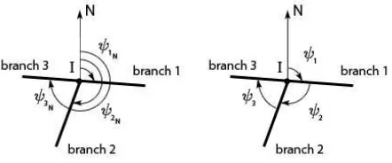
3.4.2 Road intersection feature The road intersection fea-ture modelling approach used here was adopted from Dumble [36]. Intersection descriptorI, that permits performing intersec-tion matching regardless of the posiintersec-tion and orientaintersec-tion of the feature in the camera frame, looks as follows.
I= [X, Y, Z]g, nb, ψbN, ψb, (4)
where[X, Y, Z]g
is the location of the intersection centroid in the geodetic frameFg,nbis the number of road branches,ψbN angles of the road branches forming the intersection relative to North (Fig. 9) andψb- the angular difference between the suc-cessive road branches. The width of the branches can also be added to the descriptor to improve uniqueness of the feature.
4. FEATURE LOCALISATION AND ASSOCIATION
4.1 Road network feature matching
Feature matching is the part of the visual navigation algorithm responsible for associating the features detected in the camera frame with those in a database. Improvement of both the unique-ness of features and the construction of several association levels ensures fault detection prior to feeding the feature into the navi-gational update. To optimise the computational load of the asso-ciation operation on the system, the matching tasks are prioritised and assigned to different threads, each associated with a specific
Figure 10: Pattern matching and transformation calculation for intersections detected in the camera (green dots) and database matches (black)
combination of features present in the image. Choice of data as-sociation thread depends on both type and number of features present in the camera frame. The correspondence between fea-tures present in the camera frame and the initialised data match-ing threads is shown in Table 1.
Feature combination Matching thread 1 roads and 1+ intersections intersection pattern matching 2 roads and 1 intersection intersections and splines
3 roads only splines
Table 1: Correspondence between features present in the frame and initiated association thread
The choice of features for data association is hierarchical and can be explained by differences in priority of the operations. As mentioned before, intersection matching has priority compared to spline matching because it is less computationally expensive and provides absolute information constraining the inertial drift from the IMU. Hence, if the intersection association thread initiated in the first case (Table 1.), successfully registers the pattern of in-tersections in the database, there is no need for additional spline matching. In the third case, however, when intersection asso-ciation is not possible, localisation information is derived from spline matching only. Depending on the shape of the spline, it can provide precision in one or two directions. Therefore, splines with sections of high curvature can be seen as unique features are assigned higher priority in the matching sequence over vir-tually straight splines. Future realisation of the data association algorithm will also consider water bodies and shapes formed by greenery detected in the frame in pattern analysis. Data associa-tion threads are described in the next secassocia-tion.
4.2 Road intersection matching
4.2.1 Intersection feature matching Each of the intersections detected in the camera frame is matched to the feature database based on the ECEF coordinates[Xi, Yi, Zi]g, number of branches
nb, and angles between them. Pairs of intersections for which the least-square position errorδLiand the difference of orientation of the branchesψiare lower than the corresponding thresholds are considered as a potential match. The corresponding comparison measures are defined as follows.
ni=niDB; δψi= Σni(ψi−ψiDB); (5)
δŁi= p
Σ([Xi, Yi, Zi])g−([Xi, Yi, Zi]gDB))2) (6)
Depending on the number of intersections in the frame pattern matching is initiated, which compares the angles and the distance of the polygon constructed from camera features (green dots, Fig.10) to those of the polygon constructed using their database matches (shown with black dots).
4.2.2 Intersection pattern matching At this stage the angle
ψiformed by vertexiand distance between the adjacent vertices
diis compared with the corresponding angle and distance in the polygon built based on the database information and the matches
which produce errorsδψi, δdihigher than the threshold value are rejected. Errorsδψi, δdiare defined as
δψi= Σ(ψi−ψiDB); (7)
δdi= Σ(di−dDB) (8)
The check of the angles and distances a pattern forms ensures that the detected features are located in the same plane and connection between them resembles the pattern stored in the database. After correspondence between the matched features being confirmed, the transformation between the corresponding vertices of the two polygons (Fig.10) is estimated through singular value decompo-sition to correct the camera pose. Since the offset remains con-sistent for all features in the frame, the transformation defined by rotation matrixRand translation vectortestimated via pattern matching can serve as an update for the Kalman filter. Precision of the aircraft estimate is generally sufficient to isolate possible matches within the database so, repetitive patterns and regular geometry is not considered to be a problem. If multiple possible matches cannot be discriminated, none of them will be used as innovations.
4.2.3 Road centreline matching The spline nodes accurately capture the location of the road centreline and information about the shape of the road component. It would be incorrect though to match the location of individual nodes of the splines present in the image to the ones in the database due to the non-deterministic na-ture of the procedure though which they are generated. However, spline matching can reliably use the characteristic shape of the road segment by analysing its curvature. Spline matching takes into account the peculiarity that spline features have due to aerial video as their sources: each subsequent piece of the information about the feature “enters” the frame at the top, and is added to the feature representation available from the previous frame.
Curvature-based spline matching uses algebraic curvature de-scription of the spline to search for correspondences in the database. Once the correspondence is found, the part of the feature which enters the camera field of view in the subsequent frame, is added to the match correspondingly. The spline matching procedure, depending on the shape of the road, can constrain the drift of dead reckoning in one or both directions. This leads to priority ranging of detected splines. The sections capturing grater change in curvature of a spline will have higher priority in the matching sequence since they constrain the drift in both directions in a 2D plane compared to relatively straight sections of the splines which can only limit the drift of the vehicle in a direction perpendicular to the spline. Two subsequent video frames with spline sections limiting the position drift in both directions are shown as an ex-ample in Figure 11. It is worth noting that the repeatability of the spline extraction across the frames allows reliable operation of both SLAM and database matching threads.
5. EXPERIMENTAL RESULTS
Figure 11: Splines detected in the frame (shown in yellow) com-pared to priority matching spline (green).
the error in altitude (see Fig. 14). For future processing of real UAV flight data, compensation of the range to the surface and terrain height using Digital Elevation Maps will be added to the
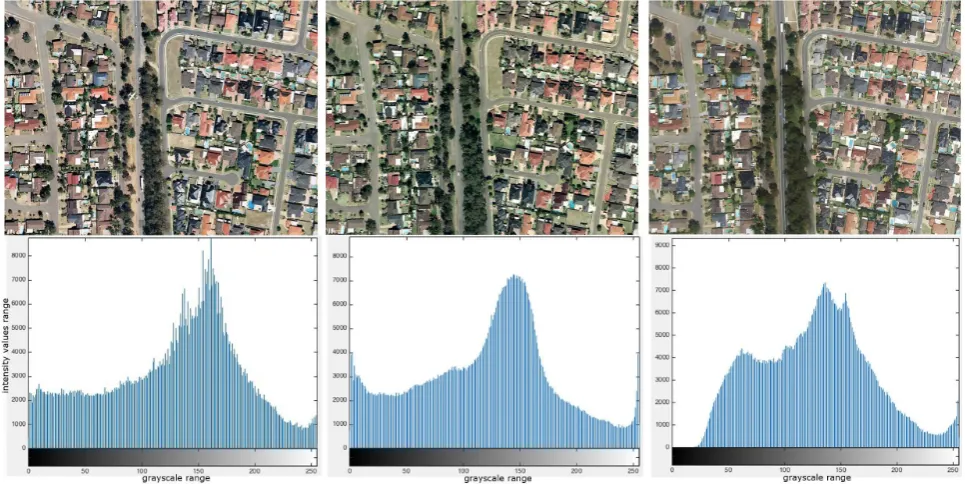
Figure 12: Combined histograms of the frame #1 from Datasets 2007, 2009, 2014 correspondingly.
Dataset Features detected Features matched Ratio
Dataset 2007 566 152 27%
Dataset 2009 166 46 27%
Dataset 2014 768 150 20%
Table 2: Comparison of number of features detected and fused in the navigation filter
algorithm.
A number of tests were conducted to evaluate the robustness of the algorithm. Three datasets based on Google Earth imagery taken in different years (2007, 2009, and 2014) closely resem-ble video that would typically be taken from an on-board down-ward looking camera, including variations in camera field of view when the vehicle is performing a coordinated turn. The three datasets were picked to represent different season, lighting con-ditions as well as to capture structural changes of the urban en-vironment (Fig. 12). All three videos were analysed by feature extraction and matching threads of the algorithm. A database of intersections used for feature matching was constructed sepa-rately by manually extracting the locations and angular orienta-tions of the road intersecorienta-tions in the fly-over area using Google Earth software. Criteria for positive matches were chosen as an-gle δψi<2◦, and distanceδŁi< δŁthr, whereδŁthr= 8[m], to ensure fusion of only true positives in the navigational Kalman filter (for description of the criteria see 4.2.1). As a planar ac-curacy measure, the distribution of distance and difference in angular orientations of matched junctions from Dataset 2007 is presented on Fig 13. The comparison of the number of features identified and matched per dataset is shown in Table 2.
Figure 13: Accepted errors in distance and angular orientation of the matched intersections shown against the number of intersec-tions.
The sections of the video between frames 90-100 and 154-180 correspond to flight over the area covered by the lake and for-est respectively. No intersections or road centrelines are detected within these sections of the video that corresponds to the period of unconstrained position drift (Fig. 14). From frame 200, the airplane enters an urban area and as soon as the positive reliable match is found, the position error drops to a value close to zero. Other peculiarities connected to the dataset account for structural changes, such as the presence of the new built-up area in frames 149-153 of the 2014 dataset, which were not present at the time of the database construction.
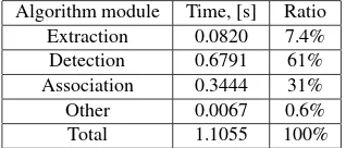
The breakdown of execution time, showing the share of each of the functions in the overall processing time of a typical 1024x768 px frame from an aerial sequence, is presented in Table 3.
Algorithm module Time, [s] Ratio
Extraction 0.0820 7.4%
Detection 0.6791 61%
Association 0.3444 31%
Other 0.0067 0.6%
Total 1.1055 100%
Table 3: Breakdown of the algorithm execution time for a typical 1024x768px video frame
Figure 14: Position error between true vehicle position and the position calculated from IMU data integrated with VNS in North, East and down directions.
Figure 15: The number of features detected and matched with the database in the videos sequences generated using Google Earth imagery from 2007, 2009, and 2014.
6. CONCLUSION
Current work shows the effective application of the designed fea-ture extraction and matching algorithm to the task of visual navi-gation. Feature extraction technique aimed to maximise the unique-ness of each detected feature and a frame as a whole. The fea-ture description and registration techniques developed use mini-mal description vector to optimise the operation of the matching system performing a continuous database search, producing reli-able periodic position update.
Testing of the algorithm performance in the presence of varying image conditions, such as changes in illumination and seasonal effect, has proved that an intensity-based classifier combined with frequency information can present a reliable robust solution for region extraction. The comparison has shown the effect of the change in intensity of the image on feature detection. The drop in the number of features detected in the most recent sequence (Dataset 2014) with least contrast resulted in less frequent nav-igational updates although with no significant loss of accuracy. The test also proved that the system operates reliably with only 20-30% of the features detected from those present in the image without drop in accuracy of the localisation solution. From the presented graphs it is evident that the localisation error drops sig-nificantly each time the features are detected and registered in the image. The database search also allows for prolonged periods with no features detected, by adapting the search region of the database according to the position uncertainty.
ACKNOWLEDGEMENTS
The author wishes to thank Dr. Steve J. Dumble and David G. Williams whose research inspired and contributed to the current work.
REFERENCES
[1] A. Cesetti, E. Frontoni, A. Mancini, P. Zingaretti, and S. Longhi, ”A vision-based guidance system for UAV navigation and safe landing using natural landmarks,” in Selected papers from the 2nd International Symposium on UAVs, Reno, Nevada, USA June 8-10, 2009, 2010, pp. 233-257.
[2] A. Marburg, M. P. Hayes, and A. Bainbridge-Smith, ”Pose Priors for Aerial Image Registration,” inInternational Confer-ence on Digital Image Computing: Techniques and Applications (DICTA), 2013, pp. 1-8.
[3] A. Cesetti, E. Frontoni, A. Mancini, P. Zingaretti, and S. Longhi, ”A Vision-Based Guidance System for UAV Navigation and Safe Landing using Natural Landmarks,”Journal of Intelli-gent and Robotic Systems, vol. 57, pp. 233-257, 2009.
[4] C. Forster, M. Pizzoli, and D. Scaramuzza, ”SVO: Fast semi-direct monocular visual odometry,” inConference on Robotics and Automation (ICRA), 2014 IEEE International, 2014, pp. 15-22.
[5] J. B. Mena, ”State of the art on automatic road extraction for GIS update: a novel classification,”Pattern Recognition Letters, vol. 24, pp. 3037-3058, 2003.
[6] H. Mayer and S. Hinz, ”A test of automatic road extraction approaches,” 2006.
[7] A. Volkova and P. W. Gibbens, ”A Comparative Study of Road Extraction Techniques from Aerial Imagery: A Navigational Per-spective,”Asia-Pacific International Symposium on Aerospace Tech-nology (APISAT), Cairns, Australia, 25 - 27 November 2015. [8] F. Bonin-Font, A. Ortiz, and G. Oliver, ”Visual Navigation for Mobile Robots: a Survey,” 2008.
[9] M. Song and D. Civco, ”Road Extraction Using SVM and Im-age Segmentation,” 2004.
[10] J. Inglada, ”Automatic recognition of man-made objects in high resolution optical remote sensing images by SVM classifica-tion of geometric image features,”ISPRS Journal of Photogram-metry and Remote Sensing, vol. 62, pp. 236-248, 2007.
[11] X. Huang and L. Zhang, ”An SVM ensemble approach com-bining spectral, structural, and semantic features for the classifi-cation of high-resolution remotely sensed imagery,”IEEE Trans-actions on Geoscience and Remote Sensing, vol. 51, pp. 257-272, 2013.
[12] X. Huang and Z. Zhang, ”Comparison of Vector Stacking, Multi-SVMs Fuzzy Output, and Multi-SVMs Voting Methods for Multiscale VHR Urban Mapping,”Geoscience and Remote Sens-ing Letters, IEEE, vol. 7, pp. 261-265, 2010.
[13] M. Zelang, W. Bin, S. Wenzhong, and W. Hao, ”A Method for Accurate Road Centerline Extraction From a Classified Im-age,”IEEE Journal of Selected Topics in Applied Earth Observa-tions and Remote Sensing, vol. 7, pp. 4762-4771, 2014. [14] C. Poullis, ”Tensor-Cuts: A simultaneous multi-type feature extractor and classifier and its application to road extraction from satellite images,”ISPRS Journal of Photogrammetry and Remote Sensing, vol. 95, pp. 93-108, 2014.
[15] Z. Sheng, J. Liu, S. Wen-zhong, and Z. Guang-xi, ”Road Central Contour Extraction from High Resolution Satellite Image using Tensor Voting Framework,” in2006 International Confer-ence on Machine Learning and Cybernetics, 2006, pp. 3248-3253.
[16] C. Cheng, F. Zhu, S. Xiang, and C. Pan, ”Accurate Urban Road Centerline Extraction from VHR Imagery via Multiscale
Segmentation and Tensor Voting,” IEEE Transactions on Geo-science and Remote Sensing, 2014.
[17] C. Wiedemann and H. Ebner, ”Automatic completion and evaluation of road networks,”International Archives of Photogram-metry and Remote Sensing, vol. 33, pp. 979-986, 2000.
[18] S. S. Shen, W. Sun, D. W. Messinger, and P. E. Lewis, ”An Automated Approach for Constructing Road Network Graph from Multispectral Images,” vol. 8390, pp. 83901W-83901W-13, 2012.
[19] A. W. Elliott, ”Vision Based Landmark Detection For Uav Navigation,”MRes Thesis, 2012.
[20] C. Steger, C. Glock, W. Eckstein, H. Mayer, and B. Radig, ”Model-based road extraction from images,” 1995.
[21] A. Barsi, C. Heipke, and F. Willrich, ”Junction Extraction by Artificial Neural Network System - JEANS,” 2002.
[22] G. Duo-Yu, Z. Cheng-Fei, J. Guo, S.-X. Li, and C. Hong-Xing, ”Vision-aided UAV navigation using GIS data,” in Vehic-ular Electronics and Safety (ICVES), 2010 IEEE International Conference on, 2010, pp. 78-82.
[23] O. Besbes and A. Benazza-Benyahia, ”Road Network Ex-traction By A Higher-Order CRF Model Built On Centerline Cliques.” [24] M. Nieuwenhuisen, D. Droeschel, M. Beul, and S. Behnke, ”Autonomous MAV Navigation in Complex GNSS-denied 3D Environments,” 2015.
[25] M. Blsch, S. Omari, M. Hutter, and R. Siegwart, ”Robust Visual Inertial Odometry Using a Direct EKF-Based Approach.” [26] Z. Miao, W. Shi, H. Zhang, and X. Wang, ”Road centerline extraction from high-resolution imagery based on shape features and multivariate adaptive regression splines,”IEEE, 2012. [27] G. Conte and P. Doherty, ”An Integrated UAV Navigation System Based on Aerial Image Matching,” p. 10, 2008.
[28] C.-F. Zhu, S.-X. Li, H.-X. Chang, and J.-X. Zhang, ”Match-ing road networks extracted from aerial images to GIS data,” in Asia-Pacific Conference on Information Processing, APCIP 2009, pp. 63-66.
[29] W. Liang and H. Yunan, ”Vision-aided navigation for air-crafts based on road junction detection,” inIEEE International Conference on Intelligent Computing and Intelligent Systems ICIS, 2009.. , 2009, pp. 164-169.
[30] J. Jung, J. Yun, C.-K. Ryoo, and K. Choi, ”Vision based navigation using road-intersection image,” in11th International Conference on Control, Automation and Systems (ICCAS), 2011, pp. 964-968.
[31] A. Dawadee, J. Chahi, and D. Nandagopal, ”An Algorithm for Autonomous Aerial Navigation Using Landmarks,”Journal of Aerospace Engineering, vol. 0, p. 04015072, 2015.
[32] R. C. Gonzalez, R. E. Woods, and S. L. Eddins, Digital Im-age processing using MATLAB. United States: Gatesmark Pub-lishing, 2009.
[33] D. G. Williams and P. W. Gibbens, ”Google Earth Imagery Assisted B-Spline SLAM for Monocular Computer Vision Air-borne Navigation.”
[34] L. Pedraza, G. Dissanayake, J. V. Mir, D. Rodriguez-Losada, and F. Matia, ”BS-SLAM: Shaping the World,” inRobotics: Sci-ence and Systems, 2007.
[35] C. Poullis and S. You, ”Delineation and geometric modeling of road networks,” inISPRS Journal of Photogrammetry and Re-mote Sensing, vol. 65, pp. 165-181, 2010.