A NEW HIGH-RESOLUTION ELEVATION MODEL OF GREENLAND DERIVED
FROM TANDEM-X
B. Wessel a, *, A. Bertram a,b, A. Gruber a, S. Bemm a,b, S. Dech a
a German Aerospace Center, German Remote Sensing Data Center, 82234 Wessling, Germany – (Birgit.Wessel, Astrid.Gruber, Stefan.Dech)@dlr.de
b
Sachverständigenbüro für Luftbildauswertung und Umweltfragen (SLU), 81243 Munich, Germany – (Adina.Bertram, Stefan.Bemm)@dlr.de
Commission VII, WG VII/2
KEY WORDS: DEM, Greenland, TanDEM-X, ICESat, penetration depth, block adjustment
ABSTRACT:
In this paper we present for the first time the new digital elevation model (DEM) for Greenland produced by the TanDEM-X (TerraSAR add-on for digital elevation measurement) mission. The new, full coverage DEM of Greenland has a resolution of 0.4 arc seconds corresponding to 12 m. It is composed of more than 7.000 interferometric synthetic aperture radar (InSAR) DEM scenes. X-Band SAR penetrates the snow and ice pack by several meters depending on the structures within the snow, the acquisition parameters, and the dielectricity constant of the medium. Hence, the resulting SAR measurements do not represent the surface but the elevation of the mean phase center of the backscattered signal. Special adaptations on the nominal TanDEM-X DEM generation are conducted to maintain these characteristics and not to raise or even deform the DEM to surface reference data. For the block adjustment, only on the outer coastal regions ICESat (Ice, Cloud, and land Elevation Satellite) elevations as ground control points (GCPs) are used where mostly rock and surface scattering predominates. Comparisons with ICESat data and snow facies are performed. In the inner ice and snow pack, the final X-Band InSAR DEM of Greenland lies up to 10 m below the ICESat measurements. At the outer coastal regions it corresponds well with the GCPs. The resulting DEM is outstanding due to its resolution, accuracy and full coverage. It provides a high resolution dataset as basis for research on climate change in the arctic.
* Corresponding author
1. INTRODUCTION
Greenland is covered by the earth’s second largest ice sheet after Antarctica with an area of about 1.7 million km² and volume of 2.85 million km³ (Tedesco et al., 2015). This volume of ice would raise the mean sea level by 7.36 m (Bamber et al., 2013). In terms of climate change and global warming, Greenland, as part of the arctic climate, plays an important role, especially in contrast to the global mean sea level change. Since the end of the last century melting/run-off phenomena came into the fore and have been increasing in the last years (van den Broeke et al., 2009). Recent studies like Groh et al. (2014) and Helm et al. (2014), mostly based on radar altimetry remote sensing techniques, analyzed melt phenomena and calculated the mass loss per year. Furthermore, the decrease of the ice sheet results in changed snow pack characteristics (Liu et al., 2006).
Several digital elevation models (DEMs) over Greenland including the ice sheet and the ice free parts exist. The first complete DEM was published in 1996, derived mostly by radar altimetry amongst others from the satellites Geosat and ERS-1 (Ekholm, 1996). The average resolution with 2 km and the accuracy of the ice sheet elevations with 12-13 m can be described as very coarse nowadays. Five years later Bamber et al. (2001a) produced a new DEM with an improved accuracy and resolution of 1 km, using the same altimetry satellites, but validated with airborne laser altimeter. Based on this Bamber et al. (2001b) published a new ice thickness and bed elevation
dataset of Greenland (5 km resolution). In 2013 it was updated, derived from multiple airborne ice thickness surveys with a better resolution (1 km) (Bamber et al., 2013). The Global DEM (GDEM) generated from Advanced Space borne Thermal Emission and Reflection Radiometer (ASTER) data has been released in 2009 with a much better resolution of about 30 m (Reuter et al., 2009). It is not a specific DEM for Greenland, but was used according to the better resolution for different analyses of ice loss (e.g. Howat et al., 2008). Version two was released in 2011. Two new high-resolution DEMs were published in 2014. The first was produced within the Greenland Ice Mapping Project (GIMP), posted at 30 m where different satellite altimetry and stereo-photogrammatic DEMs were used to enhance the existing DEM of Bamber et al. (2001a). The validation with ICESat tracks shows greater uncertainties over ice free (+/-18.3 m) and outer melting regions than over the inner ice sheet (+/-8.5 m). The second DEM was derived from the altimeter on board of the CryoSat-2 satellite, and Helm et al. (2014) additionally presented the first elevation change map of Greenland between 2011 and 2014. Based on these DEMs different ice mass loss studies of Greenland were conducted (e.g. Groh et al., 2014; Hanna et al., 2013; Van den Broeke et al., 2009).
from the opposite viewing geometry. The first global coverage was acquired mainly in winter 2010/2011 and the second mainly in 2011/2012. Crossing and missing acquisitions were acquired until mid-2014. The primary goal of the TanDEM-X mission is the derivation of a global DEM. The double and more coverages are aiming to achieve a random height error of 2 m. An absolute height error of 10 m is specified.
In order to obtain the high quality of the TanDEM-X DEM world-wide, a significant instrument and system calibration effort was carried out (Hueso González et al., 2012). However some systematic height errors remain. Especially, offsets and tilts in range and azimuth in the order of few meters and some decimetres respectively are present. The nominal estimation of these height errors is conducted within a least-squares adjustment with ICESat (Ice, Cloud, and land Elevation Satellite) laser measurements serving as ground control points (GCPs). But for Greenland with its large ice sheet this procedure would lead to an uplift or even deformation of the DEM to surface reference data: X-Band SAR penetrates snow and ice up to ten meters ,whereas, laser measurements represent the real surface. To avoid this discrepancy a special strategy of the least-squares adjustment of individual DEM scenes is presented. The resulting DEM could improve current estimates of the Greenland ice sheet mass loss and could help to monitor spatial and temporal changes. It is a high resolution dataset providing a basis for research on climate change in the arctic.
In this paper we present a new DEM of Greenland, which is based on more than 3.5 years of TanDEM-X DEM acquisitions. In the following, we first describe the used data (chapter 2) and the ice-sheet adopted procedure to generate the DEM (chapter 3). The resulting DEM and comparisons with absolute height reference data are presented in chapter 4. Chapter 5 concludes the paper and gives an outlook.
2. DATA 2.1 TanDEM-X data
The data used are interferomtric SAR acquisitions from the TanDEM-X mission. The operational TanDEM-X DEM acquisitions are performed using the bistatic Stripmap mode in single horizontal polarization. According to the acquisition plan (Borla Tridon et al., 2013) the time span to cover Greenland adequately with TanDEM-X data took nearly 4 years. First and second year coverages were taken in winter 2010/2011 and 2011/2012. In addition, for the steep coasts a third and a fourth coverage from the opposite viewing geometry were performed until mid-2014. On the one hand there is a very good coverage, but on the other hand due to the greater time span there are also a lot of changes in the elevation caused by melting as well as by varying scattering characteristics over time.
2.2 ICESat GLA14 elevation data
For block adjustment as well as for comparison we use data of the Ice, Cloud, and land Elevation Satellite (ICESat) mission. The Geo-science Laser Altimeter System (GLAS) aboard of ICESat is a laser altimeter system that measures the Earth surface along profiles with an along-track sampling of 170 m and a footprint of ~ 70m. ICESat is characterized by its high accuracy and high global spatial coverage of altimeter measurements. The data cover the time span from 2003 to 2009 (Zwally et al., 2011). The used centroid heights were referenced
to WGS84 and corrected for errors (e.g. cloud flag). In addition, a filtering was applied to select only reliable points on the bare and flat surface (Huber et al., 2009).
The main problem for an adjustment of InSAR DEMs over Greenland is that the phase center does not correspond with the physical surface that the GCPs normally refer to. The used GCPs – the ICESat GLA14 points – are obtained from laser altimeter measurements that reflect exclusively the surface. So, before starting with the adjustment two questions have to be clarified: a) to what surface shall the DEM be referenced and b) how or to which (selection of) GCPs shall this be realized?
2.3 X-Band reflective surface of Greenland
The Greenland surface consists of rocks in the outer coastal zone and of snow and ice in the inner zone. Based on Benson’s (1962) snow zone model for Greenland four distinct surface areas of an ice sheet or glacier (facies) are subdivided: the superimposed (bare) ice zone, the wet (soaked) snow zone, the percolation zone, and the dry snow zone (Lui et al. 2006, see Figure 1 and Figure 2).
Figure 1. Schematic representation of different snow zones, from Lui et al., 2006
In each snow zone different snow characteristics predominate depending on snow grain size and density, layer succession, surface roughness, and water content of snow. These factors affect the brightness of the backscatter and the penetration of the SAR signal. Thereby, also the portion of surface and volume backscattering depends on these factors. Several studies characterized the SAR backscattering for each zone separately:
The dry snow zone is located in the high interior of Greenland. Here, normally no melting occurs. This leads to a relative low density of the cold snow pack. The fine grain size causes little volume scattering (Fahnestock et al. 1993; Ashcraft and Long, 2005; Liu et al., 2006; Picard and Fily, 2006). This evokes the highest penetration depth. The backscatter of the reflected signal is very low in the dry snow zone.
Percolation zone: The inner dry snow zone of Greenland is surrounded by the percolation zone (Benson et al. 1962). It is characterized by some amount of melt, which causes snow grains, subsurface ice pipes and horizontal lenses in the order of some centimeters to tens of centimeters (Jezek et al., 1994; Ashcraft and Long, 2005; Liu et al., 2006; Weber Hoen and Zebker, 2000). The surface scattering on those grains leads to a relatively bright backscatter with less penetration.
The wet snow zoneis hard to distinguish from the percolation zone, because the scattering mechanisms are nearly the same. Though, compared to the percolation zone strong melt phenomena occur during summer and lead to a higher variability. This zone is also characterized by the presence of multiple ice layers and is located further down slope towards the coast of Greenland (Ashcraft and Long, 2005; Benson 1962; Rignot et al., 1993).
Ablation zone is the outer coastal region. It is characterized by surface mass loss caused by runoff. During warm summers the snow pack completely melts, which leads to a surface of bare ice and rock (Ashcraft and Long, 2005; Hanna et al., 2013). Here the backscatter of the radar signal is due to the high water content strongly decreased with minimal penetration depth (Weber Hoen and Zebker, 2000).
In general the acquisitions were taken in winter because they are free from the complicating presence of meltwater. Nevertheless, there are some summer scenes that reduce the backscatter at lower elevations.
2.4 Exemplarily analysis of real data
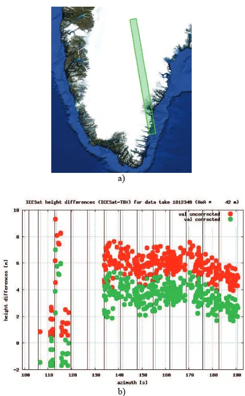
To investigate the behaviour of the penetration depth of the X-Band InSAR DEM acquistions, the height differences between ICESat and TanDEM-X data were analysed. Figure 3 shows a typical adjustment of the height differences: DEM scenes in Figure 3 are separated by vertical black lines. The line distance is approximately 50km. The red dots represent the differences before the adjustment. Here an offset of -2.3 m was estimated by the least-squares adjustment. The differences corrected by the offset are plotted in green. Coming from the outer rock zone the differences of the first two DEM scenes of datatake 1012340 are around zero. In the percolation zone, from scene 6 on, the differences increase rapidly. The green dots in Figure 3 show clearly an almost constant value around 4 m. The beginning of the percolation zone is clearly visible. There are only marginal variations of penetration depth within the percolation zone.
a)
b)
Figure 3. a) Datatake 1012340 starting from rock towards percolation zone, b) Differences between ICESat and TanDEM-X heights of datatake 1012340: in red before and in green after the block adjustment
3. NEW DEM ADJUSTMENT APPROACH FOR GREENLAND
3.1 General block adjustment approach for TanDEM-X data
In order to correct the remaining systematic errors described in the introduction a least-squares block adjustment as presented in Gruber et al. (2008) is applied. Therefore, the following error function is set up:
az
(offset, tilt in range and tilt in azimuth)rg, az = image coordinates, i.e. ground distance (range) and azimuth with respect to a reference point.
heights can be directly compared in the overlap area of neighbouring DEM acquisitions. For each ICESat and tie-point height difference the observation equations are derived as follows:
∆
= adjusted height difference between ICESat and TanDEM-X DEMK J
H
ˆ
,∆
= adjusted height difference for tie-pointsApplying this method, the correction parameters can be found independently from the terrain. Estimated offsets and tilts are applied during the subsequent step of the so-called mosaicking.
3.2 Block adjustment approach for Greenland
This calibration approach described in the previous section is applied and validated for three-quarter of the whole globe. However, in Greenland one has to deal with more difficult conditions: First of all due to ice melting within the acquisition time span, the tie-points may represent different height values. Also, the heights in general may be affected by more random noise, as the coherence over wet snow is worse. In addition the penetration of the SAR signal varies significantly for different snow facies. Therefore, in some cases the height differences seem to be affected by systematic effects which are not caused by remaining errors but by different surface conditions. Considering that tilts are only some decimeters whereas change of snow depth, random noise and variations due to different penetration depth can result in several meters of height differences, tilts can hardly be estimated. For these reasons only offsets are estimated for Greenland.
However even the offsets cannot be estimated by the standard calibration approach using all available ICESat points, as the penetration of ICESat differs by up to 10 m from the penetration of SAR. The elevation of the natural phase center should be preserved to avoid any further deformation. The resulting DEM should represent the X-Band reflective surface (Wessel, 2013).
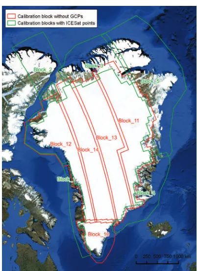
Therefore, Greenland is divided into 13 adjustment blocks: The adjustment blocks 1-5 (see Figure 4) are located in the outer coastal zone where rock predominates and are calibrated first. In these blocks ICESat points are used as GCPs. In contrast, blocks 10-14 are within the snow zones, where the penetration depth of radar and ICESat differs strongly. In order to avoid deformation towards ICESat, blocks 10-14 are successively adjusted according to their numbering and just connected by the tie-points with each other. Hereby the tie-points of the datatakes which are already calibrated serve as GCPs.
Figure 4. Blocks for adjustment of Greenland: green adjustment to ICESat, red: adjustment by tie-points with no ICESat points
4. RESULTS
Looking at the adjustment results, the interferometric DEMs show a very clear development: After the block adjustment, over rock the differences to the GCPs are near zero, as shown by DEM scene 1012340_2 and 1012340_3 in Figure 3. Also notable is the fact that the differences between overlapping datatakes go around zero in Figure 5. The differences over rock have larger variances as expected (see azimuth 105 – 120 in Figure 5). But surprisingly the values over snow and ice stay very homogenous (see azimuth 135 – 190 in Figure 5).
Figure 5. Tie-points starting from rock towards percolation zone of datatake 1012340: Differences master datatake – neighboring
The variation of one datatake pair is below 0.5 m. All overlapping datatakes are within a band of 2 m. But the datatakes are adjusted to the same height level that means residual respectively natural height offsets remain. Reasons for those smaller height differences are possibly changing backscatter conditions, change of the surface, or different acquisition parameters like the height of ambiguity. In the example datatake of Figure 5, a similar penetration with similar height of ambiguity datatakes is observed. All heights of ambiguity are around 42 m. Other datatakes show larger differences when dealing with more different heights of ambiguities.
Finally, all 7414 DEM scenes were mosaicked with a robust mosaicking approach taking into account height discrepancies (Gruber et al., 2016), see Figure 7a. The ellipsoidal heights of the resulting DEM of Greenland go from sea level up to 3797 m. Taking into account that the penetration in the area of the top is around 8 m, the highest peak would be around 3805 m. Remarkable is that the plateau of the highest elevation (at 72° North) is not located in the zone with the highest penetration depth compared to ICESat data (at 78° North, see Figure 7a and Figure 6). This refutes former theories that the largest penetration occurs at the highest altitudes (Benson, 1962).
In contrast to other parts of the world, during the Greenland DEM processing a certain amount of DEM scences had to be rejected during block adjustment. Partly DEMs were rejected (200 scenes, 2.5%) e.g. due to unsolved height offsets in the order of the height of ambiguity. The correct determination within the adjustment was more problematic in a variing snow and ice environment. However, in order to avoid gaps in the final DEM, partly problematic DEM scenes were used for the mosaic in case of no other available coverage (300 scenes, 4.0%).
Figure 8b displays the corresponding height error map (HEM). The height error increases to the inner part of Greenland. Also the different acquisition contributions are visible: The fewer acquisitions overlap, the larger (brighter) is the height error (Figure 8a and 8b). From regions covered several times to regions covered less, steps in the mosaicked DEM may occur. Those different height levels may be caused by seasonal variations of snow and ice. In regions covered several times, these effects are reduced by averaging. As stated before, the DEM acquisitions are not forced completely to each other; natural changes are preserved by the adjustment. But incompatible DEM scenes that provoke larger edges in the DEM were iteratively eliminated by an operator to finally obtain a homogenous DEM. However, to avoid gaps in the Greenland DEM smaller steps below 1 m were accepted.
4.1 Comparison with ICESat GLA14 elevations
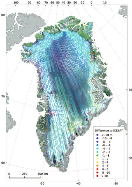
For quality assessment the new DEM is compared to ICESat points covering the period from 2003 to 2009 resulting in around 7 million, well distributed reference points. The overall mean difference between the new DEM and ICESat is -3.97 m with a standard deviation of 3.23 m. This proves that most parts of the new Greenland DEM are below the surface as expected. For a more detailed analysis the differences between the DEM and the ICESat tracks are plotted in Figure 6.
Figure 6. Amplitude mosaic superimposed with color-coded height differences TanDEM-X – ICESat
The differences can be classified into the facies described in section 2.3. For the coastal rock region most differences range between -1 and 1 m. The green points over rock clearly state that the adjustment on the outer rocks worked very well. But there are also some parts in the ablation zone with a difference below -10 m. These height changes in the western and southern part of Greenland are particularily observable over the pure ice surface. This fact is equal to the findings of Groh et al. (2014), Helm et al. (2014) and Sørensen et al. (2011).Here
probably a decrease of larger glacier parts took place. The percolation zone (comparing the facies in Figure 2 and Figure 6) shows mainly differences between -1 m and -4 m. Especially in the northern part the transition from the percolation zone to the dry snow zone is obvious. The differences go immediately into the darker blue values representing height differences of up to 10m. The dry snow zone is also visible in the mean amplitude mosaic characterized by a low backscatter in Figure 8b. Note that the amplitude values are not calibrated.
Figure 7. a) DEM of Greenland based on TanDEM-X acquisitions with color-coded elevations; b) mean amplitude mosaic
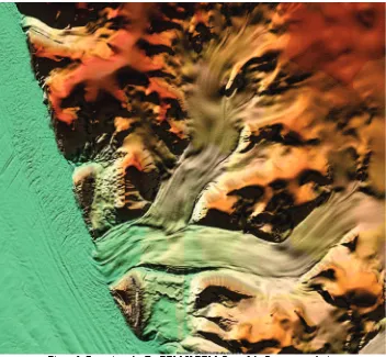
Figure 9. Zoom into the TanDEM-X DEM: Part of the Petermann glacier
5. CONCLUSION & OUTLOOK
In this paper we presented a new DEM derived from TanDEM-X data acquired between December 2010 and July 2014. For the first time interferometric X-band SAR data were used for a complete mapping of Greenland. The resolution of 12 m is until now the best compared to other existing DEMs of Greenland posted at 30 m (Helm et al., 2014; Howat et al., 2014). The presented block adjustment for individual DEM acquisitions worked well: in the coastal rock regions the final DEM mosaic corresponds well with ICESat elevations. Whereas in the inner part the penetration of X-Band SAR into the ice and snow pack of up to 10 m is preserved. The resulting high-resolution DEM provides a basis for different research topics related to climate change in the arctic. It could improve current estimates of the Greenland ice sheet mass loss and could help to monitor spatial and temporal changes. Direct comparisons with older data sets are possible, for example with the 30 m mosaic of ERS-1 amplitude imagery changes in the ice facies in the last 20 years might be detectable.
Nevertheless, some height errors in the dataset remain. This is due to 3.5 years of data acquisition, including different seasons. The ice mass loss over the acquisition period changed the elevation, which is visible especially in the wet snow and ablation zone in west and south-east Greenland. This fact is equal to the findings of Groh et al. (2014), Helm et al. (2014) and Sørensen et al. (2011).
Moreover, one has to be aware that the TanDEM-X DEM does not reflect the real surface elevation over some snow facies, due to a deeper penetration depth of radar. With a model of the penetration depth in every snow facies one could deviate the
surface elevation (Weber Hoen and Zebker, 2008). Then, a proper classification of the different facies would allow estimating the X-band penetration depth into the ice sheet (Rizzoli, 2016) and afterwards, if needed, the DEM could be lifted to the physical surface.
Though, the characteristics of the new Greenland DEM derived from TanDEM-X data are known, the dataset is outstanding due to its resolution, accuracy and full coverage.
ACKNOWLEDGEMENTS
The TanDEM-X project is partly funded by the German Federal Ministry for Economics Affairs and Energy (Förderkennzeichen 50 EE 1035).
REFERENCES
Ashcraft, I.S., Long, D.G., 2005. Observation and characterization of radar backscatter over Greenland. IEEE Transactions on Geoscience and Remote Sensing, 43(2), pp. 225-237.
Bamber, J.L., Ekholm, S., Krabrill, W.B., 2001a. A new, high-resolution digital elevation model of Greenland fully validated with airborne laser altimeter data. Journal of Geophysical Research, 106, pp. 6733–6745.
Bamber, J.L., Griggs, J. a., Hurkmans, R.T.W.L., Dowdeswell, J. a., Gogineni, S.P., Howat, I., Mouginot, J., Paden, J., Palmer, S., Rignot, E., Steinhage, D., 2013. A new bed elevation dataset for Greenland. The Cryosphere, 7, pp. 499–510.
Benson, C. S., 1962. Stratigraphic studies in the snow and firn of the Greenland ice sheet. U.S. Army Corps Eng., Hannover, NH, SIPRE Res. Rep. 70, pp. 1-188.
Borla Tridon, D., et al., 2013. TanDEM-X: DEM acquisition in the third year era. Int. J. Space Sci. Eng., 1(4), pp. 367–381.
Ekholm, S., 1996. A full coverage, high-resolution, topographic model of Greenland computed from a variety of digital elevation data. Journal of Geophysical Research, 101, 21,961-21,972.
Fahnestock, M. Bindschadler, R., Kwok, R., and Jezek, K., 1993. Greenland ice sheet surface properties and ice dynamics from ERS-1 SAR imagery. Science, 262, pp. 1530 – 1534.
Groh, A., Ewert, H., Fritsche, M., Rülke, A., Rosenau, R., Scheinert, M., Dietrich, R., 2014. Assessing the Current Evolution of the Greenland Ice Sheet by Means of Satellite and Ground-Based Observations. Survey of Geophysics, 35, pp. 1459–1480.
Gruber, A., Wessel, B., Martone, M., and Roth, A. 2016. The TanDEM-X DEM Mosaicking: Fusion of Multiple Acquisitions Using InSAR Quality Parameters. IEEE J. Sel. Top. Appl. Earth Obs. Remote Sens., 9(3), 1047–1057.
Gruber, A., Wessel, B., Huber, M., and Roth, A. 2012. Operational TanDEM-X DEM calibration and first validation results. ISPRS J. Photogramm. Remote Sens., 73, pp. 39–49.
Hanna, E., Navarro, F.J., Pattyn, F., Domingues, C.M., Fettweis, X., Ivins, E.R., Nicholls, R.J., Ritz, C., Smith, B., Tulaczyk, S., Whitehouse, P.L., Zwally, H.J., 2013. Ice-sheet mass balance and climate change. Nature, 498, pp. 51–59.
Helm, V., Humbert, A., Miller, H., 2014. Elevation and elevation change of Greenland and Antarctica derived from CryoSat-2. The Cryosphere, 8(4), pp. 1539–1559.
Howat, I.M., Smith, B.E., Joughin, I., Scambos, T.A., 2008. Rates of southeast Greenland ice volume loss from combined ICESat and ASTER observations. Geophysical Research Letters. 35, L17505:1-5.
Hueso González, J., Antony J.W., Bachmann, M., Krieger, G., Zink, M., Schrank, D. Schwerdt, M. 2012. Bistatic system and baseline calibration in TanDEM-X to ensure the global digital elevation model quality. ISPRS Journal of Photogrammetry and Remote Sensing, 73, pp. 3-11.
Jezek, K.C., Gogineni, P., Shanableh, M., 1994. Radar measurements of melt zones on the Greenland Ice-Sheet. Geophysical Research Letters, 21(1), pp. 33-36.
Lui, H., Wang, L., Jezek, C., 2006. Automated Delineation of Dry and Melt Snow Zones in Antarctica using active and passive microwave observations from space. IEEE Transactions on Geoscience and Remote Sensing, 44(8), pp. 2152-2163.
Picard, G., Fily, M., 2006. Surface melting observations in Antarctica by microwave radiometers: Correcting 26-year time
series from changes in acquisition hours. Remote Sensing of Environment, 104, pp. 325–336.
Reuter, H.I., Nelson, A., Strobl, P., Mehl, W., Jarvis, A., 2009. A first assessment of Aster GDEM tiles for absolute accuracy, relative accuracy and terrain parameters. In: Geoscience and Remote Sensing Symposium, 2009 IEEE International, IGARSS 2009, Cape Town, pp. 240–243.
E. Rignot; K. Jezek; J.J. van Zyl; M.R. Drinkwater: Radar scattering from snow facies of the Greenland ice sheet: results from the AIRSAR 1991 campaign, In: IEEE Geoscience and Remote Sensing Symposium, 18-21 Aug. 1993, Tokyo (JP), pp. 1270-1272.
Rignot, E., Jezek, K., van Zyl, J.J., Drinkwater, M.R., 1993: Radar scattering from snow facies of the Greenland ice sheet: results from the AIRSAR 1991 campaign. IEEE Geoscience and Remote Sensing Symposium, Tokyo, 3, pp. 1270-1272.
Rizzoli, P., Martone, M., Bräutigam, B., 2015. Greenland ice sheet snow facies identification approach using TanDEM-X interferometric data. In: Proceedings of IGARSS, pp. 2060-2063.
Schubert, A., Jehle, M., Small, D., and Meier, E., 2008. Geometric validation of TerrraSAR-X high-resolution products. In: Proceedings of 3. TerraSAR-X Science Team Meeting, 25. - 26.11.2008, Oberpfaffenhofen, Germany.
Sørensen, L. S., Simonsen, S. B., Nielsen, K., Lucas-Picher, P., Spada, G., Adalgeirsdottir, G., 2011. Mass balance of the Greenland ice sheet (2003-2008) from ICESat data - The impact of interpolation, sampling and firn density. The Cryosphere, 5, pp. 173-186.
Tedesco, M., Box, J.E., Cappelen, J., Fettweis, X., Mote, T., Wal, R.S.W. van de, Smeets, C.J.P.P., Wahr, J., 2015. Arctic Report Card - Greenland Ice Sheet. National Oceanic and Atmospheric Administration, Washington DC, USA http://www.arctic.noaa.gov/reportcard/greenland_ice_sheet.html (07. Dec. 2015).
Van den Broeke, M.R., Bamber, J.L., Ettema, J., Rignot, E.J., Schrama, E.J., van de Berg, W., van Meijgaard, E., Velicogna, I., Wouters, B., 2009. Towards resolving recent Greenland mass loss (Invited). AGU Fall Meet. Abstr. 326, pp. 984–986.
Weber Hoen, E., Zebker, H.A., 2000. Penetration depths inferred from interferometric volume decorrelation observed over the Greenland ice sheet. IEEE Transactions on Geoscience and Remote Sensing, 38, pp. 2571–2583.