ITERATIVE RE-WEIGHTED INSTANCE TRANSFER FOR DOMAIN ADAPTATION
A. Paul∗, F. Rottensteiner, C. Heipke
Institute of Photogrammetry and GeoInformation, Leibniz Universit¨at Hannover, Germany (paul, rottensteiner, heipke)@ipi.uni-hannover.de
Commission III, WG III/4
KEY WORDS:Transfer Learning, Domain Adaptation, Logistic Regression, Machine Learning, Knowledge Transfer, Remote Sensing
ABSTRACT:
Domain adaptation techniques in transfer learning try to reduce the amount of training data required for classification by adapting a classifier trained on samples from a source domain to a new data set (target domain) where the features may have different distributions. In this paper, we propose a new technique for domain adaptation based on logistic regression. Starting with a classifier trained on training data from the source domain, we iteratively include target domain samples for which class labels have been obtained from the current state of the classifier, while at the same time removing source domain samples. In each iteration the classifier is re-trained, so that the decision boundaries are slowly transferred to the distribution of the target features. To make the transfer procedure more robust we introduce weights as a function of distance from the decision boundary and a new way of regularisation. Our methodology is evaluated using a benchmark data set consisting of aerial images and digital surface models. The experimental results show that in the majority of cases our domain adaptation approach can lead to an improvement of the classification accuracy without additional training data, but also indicate remaining problems if the difference in the feature distributions becomes too large.
1. INTRODUCTION
Supervised classification of images and derived data for auto-matic information retrieval is an important topic in photogramme-try and and remote sensing. One problem related to the machine learning techniques used in this context is the necessity to pro-vide a sufficient amount of representative training data. Whereas the use of training data allows such methods to adapt to the spe-cific distributions of features in varying scenes, the acquisition of training data, in particular the generation of the class labels of the training samples, is a tedious and time-consuming manual task. Applying a trained classifier to another image than the one from which the training data were generated reduces the amount of manual labour, but this strategy is also very likely to give sub-optimal results. This is due to the fact that in the new image the features may follow a different distribution than in the original one, so that the assumption of the training data being representa-tive for the data to be classified is no longer fulfilled. The ques-tion of how a classifier trained on one data set can be of help in another learning task is dealt with in approaches for Trans-fer Learning(TL) (Thrun and Pratt, 1998; Pan and Yang, 2010). In TL, one tries to adapt a classifier trained on samples from a
source domainto data from atarget domain. These domains may be different, but they have to be related for this type of transfer to be possible. There are different settings for the TL problem; in the context of the classification of remote sensing images we are mostly interested in the case where labelled training data are only available for the source domain, which is related to the transduc-tive transfer learningparadigm.
In this paper, we address one specific setting of transductive trans-fer learning calleddomain adaptation(DA) in which the source and the target domains are supposed to differ by the marginal distributions of the features used in the classification process, e.g. (Bruzzone and Marconcini, 2009). The particular applica-tion we are interested in is the pixel-based classificaapplica-tion of im-ages and Digital Surface Models (DSM). We use multiclass
lo-∗Corresponding author
gistic regression (Bishop, 2006) for classification. The classifier is trained on an image for which training data are available and which corresponds to the source domain in the TL framework. When a new image is to be classified, the classifier is iteratively adapted to the distribution of the features in that image, which, thus, corresponds to the target domain. This DA process is based on an iterative replacement of training samples from the source domain by samples from the target domain which receive their class labels (semi-labels) from the current version of the clas-sifier. Our method is inspired by (Bruzzone and Marconcini, 2009), but it uses logistic regression rather than Support Vec-tor Machines (SVM) as a base classifier, which is supposed to make it faster in training and classification. An initial version of our approach was found to have considerable problems in case of strong overlaps between the feature distributions of different classes (Paul et al., 2015). In this paper we expand this method so that it becomes more robust with respect to overlapping feature distributions, and we evaluate the new method using a subset of the ISPRS 2D semantic labelling challenge (Wegner et al., 2016).
This paper is organized as follows. Section 2 gives an overview on related work in transfer learning in the framework of DA, with a focus on applications in remote sensing. In Section 3 we de-scribe our new methodology for DA, whereas Section 4 presents our experimental evaluation. We conclude the article with a sum-mary and an outlook on future work in Section 5.
2. RELATED WORK
According to Pan and Yang (2010), a domainD={X, P(X)} consists of a feature spaceX and a marginal probability distri-butionP(X)withX ∈ X. In TL, we consider two domains, the source domainDSand the target domainDT. Given a
spe-cific domainD, a taskT ={C, f(·)}consists of a label spaceC, representing objectclasses, and a predictive functionf(·). This function can be learned from the training data{xi, Ci}, where
xi∈XandCi∈ C. Here again, a distinction is made between a
is defined as a procedure that helps to learn the predictive function fT(·)inDTusing the knowledge inDTandDS, where either the
domains or the tasks, or both, are different but related. There are three settings of TL (Pan and Yang, 2010). Ininductive TL, the domains are assumed to be identical, but the tasks to be solved in these domains are different(DS =DT,TS̸=TT). In contrast,
in thetransductive TLsetting, the tasks are assumed to be identi-cal, but the domains may be different(DS̸=DT,TS=TT). In
the case ofunsupervised TL, both, the tasks and the domains may be different(DS ̸=DT,TS ̸= TT). For a thorough review of
TL techniques, refer to (Pan and Yang, 2010). We are concerned primarily with the transductive setting and more specifically with DA techniques for remote sensing not requiring training data in the target domain.
According to Bruzzone and Marconcini (2009), one can distin-guish two TL scenarios in which the distributions of the features used for training (source domain) and for testing (target domain) do not match. In the first scenario, the two domains and, thus, the distributions are considered to be identical, but the training data are not representative and do not allow a sufficiently good estima-tion of the joint distribuestima-tion of the data and the classes. Depend-ing on the nature of the differences between the estimated distri-butions and the true ones, this problem is referred to assample selection bias(Zadrozny, 2004) orcovariate shift(Sugiyama et al., 2007). It is the second scenario calleddomain adaptationwe are interested in. Here, the source and target data are drawn from different domains, and the two domains differ in the marginal distributions of the features and posterior class distributions, thus P(XS) ̸= P(XT)andP(CS|XS) ̸= P(CT|XT) (Bruzzone
and Marconcini, 2009). Contsequently, techniques for impor-tance estimation such as (Sugiyama et al., 2007) can no longer be applied. Note that this definition of DA, which is adopted in this paper, is different from (Pan and Yang, 2010), where in the DA scenario the posteriors are assumed to be identical. From the point of view of our application, DA corresponds to a prob-lem where the training (source domain) data are extracted from another image than the test (target domain) data in which the dis-tribution of the features and the class posteriors are different, e.g. due to different lighting conditions or seasonal effects. Finding a solution to the TL problem in this scenario implies that one can transfer a classifier trained on one image data set to a set of simi-lar images (i.e. to a related domain in the context of DA) without having to define training data in the new images.
There are two groups of DA methods which can be differenti-ated according to what is actually transferred (Pan and Yang, 2010). The first group of methods is based on feature repre-sentation transfer. Such methods try to find feature represen-tations that allow a simple transfer from the source to the target domain, e.g. (Gopalan et al., 2011). The purpose is to obtain a set of shared and invariant features, for which the differences in the marginal and joint distributions between the two domains are minimized. Once this mapping has been established, the feature samples from both domains can be transferred to the joint rep-resentation, thus allowing the application of the classifier trained on source data in the transformed domain without any adaptation. An unsupervised feature transfer method based on feature space clustering and graph matching is proposed in (Tuia et al., 2013). Experiments based on synthetic and real data show good results. However, graph matching relies on an initial cross-domain graph containing all possible matches between cluster centroids in the two domains, and the authors conclude that their method might not work if the correct matches are not contained in that graph. In (Tuia et al., 2014), graph matching is expanded for so-called semi-supervised manifold alignment, which leads to an improved classification performance. However, this method requires
la-belled samples from all domains to provide some supervision for the graph matching process. In (Tuia, 2014), this requirement is relaxed under the assumption that the images have a certain spa-tial overlap, in which case one can identify corresponding points (semantic tie points) which provide the required labels across do-mains. However, spatial overlap is a relatively strong prerequisite that is not met in our application. Another approach for feature representation transfer based on graph matching is proposed in (Banerjee et al., 2015). The method can also deal with differ-ent class structures in the two images. However, experimdiffer-ents are only presented for multitemporal data sets of the same image re-gion; the authors’ claim that their method can also be applied in other settings is not supported by an empirical evaluation. The semi-supervised method for DA developed in (Cheng and Pan, 2014) uses linear transformations characterised by a set of rota-tion matrices for feature representarota-tion transformarota-tion. However, it also requires a small amount of representative labels from the target domain.
the semi-labels of the unlabelled data are determined according to the cluster membership of EM. Unlike our approach, this method assumes the labelled and the unlabelled data to follow the same distribution, so that no labelled training data are excluded in the training process.
In our previous work (Paul et al., 2015) we proposed a method for instance transfer that was inspired by Bruzzone and Marconcini (2009). We used a discriminative probabilistic classifier of lower computational complexity, which should also require fewer train-ing samples than a generative approach. We followed the same strategy of gradually replacing source training samples by target samples, but using logistic regression as the base classifier. This required a new strategy for deciding which source training sam-ples are to be eliminated from the training data and which samsam-ples from the target domain are to be added into the current training data set. We proposed two different strategies for that purpose. However, both had problems with overlapping feature distribu-tions. One of the main reasons for failure was the binary nature of the inclusion of target samples into or the removal of source features from the training data set in the DA process. In partic-ular, the inclusion of a training sample having a high impact on the decision boundaries (aleverage point) could lead to a sudden change in the decision boundary, which made the DA procedure unstable. In order to overcome this problem, we expanded our methodology so that it can consider individual weights in the DA process, modulating the impact on the basis of a sample’s dis-tance from the decision boundary. This allows the exclusion of uncertain feature samples by setting their weights to lower values and thus to avoid drifting of our model parameters. Additional stability is achieved by using the current state of the classifier for regularisation rather than a generic prior that assumes the ex-pected value of the parameters to be zero. This regularisation method is inspired by Kuznetsova et al. (2015), where, however, it is used in a different context. Unlike in (Paul et al., 2015), we use real data including real changes in the feature distributions for the evaluation of our new method in order to assess its potential, but also its limitations.
3. METHODOLOGY
In this section we describe our new method for TL based on mul-ticlass logistic regression. We start with the theory of logistic re-gression based on (Bishop, 2006), before presenting our approach for domain adaptation in section 3.2.
3.1 Logistic Regression
Logistic regression is a discriminative probabilistic classifier that directly models the posterior probabilityP(C|x)of the class la-belsCgiven the datax. In the multiclass case we distinguishK classes, i.e.C ∈ C={C1
, . . . , CK}
. A feature transformation into a higher-dimensional space is applied to achieve non-linear decision boundaries. That is, logistic regression is applied to a vectorΦ(x)whose components are functions ofxand whose di-mension is typically higher than the didi-mension ofx. The first element ofΦ(x)is assumed to be a constant with value 1 for sim-pler notation of the subsequent equations. In the multiclass case, the model of the posterior is based on the softmax function:
p(C=Ck|
wherewkis a vector of weight coefficients for a particular class
Ck
. As the sum of the posterior over all classes has to be 1, these
weight vectors are not independent. This is considered by setting the first weight vectorw1to0.
The parameters to be determined in training are the weightswk
for all classes exceptC1
, which can be collected in a parameter vectorw = (wT
2, . . . ,w
T K)
T
. For that purpose, a training data set, denoted as T D, is assumed to be available. It consists of N training samples(xn, Cn) withn ∈ {1, . . . , N}, wherexn
is a feature vector andCnits corresponding class label. In
ad-dition, we define a weightgn for each training sample. In the
standard setting, we usegn = 1∀n, but in the DA process, the
training samples will receive individual weights (cf. Section 3.2). Training is based on a Bayesian estimation of these parameters, determining the optimal values ofwgivenT D, by optimising the posterior (Vishwanathan et al., 2006; Bishop, 2006):
p(w|T D)∝p(w)·∏
is defined in equation 1. The indica-tor variabletnktakes the value 1 if the class labelCnof training
samplenisCk
and zero otherwise. Compared to the standard model for multiclass logistic regression, the only difference is the use of the weightsgnin the exponent, which can be motivated in
an intuitive way by the interpretation of the weights as an indica-tor for multiple instances of the same training sample, although we do not use integer values for these weights. Maximising the posterior in equation 2 is equivalent to minimising the negative logarithmE(w)of the posterior:
E(w) =−∑ ond term models the priorp(w)as a Gaussian with meanw¯and standard deviationσ, used to avoid overfitting (Bishop, 2006).
We use the Newton-Raphson method for finding the minimum of E(w). Starting from initial valuesw0
= ¯w, the updated parame-terswτin iterationτare estimated according to:
wτ =wτ−1
+H−1
∇E(wτ−1), (4)
where∇E(wτ−1)andHare the gradient and the Hessian
ma-trix of E(w), respectively, both evaluated at the values from
the previous iteration, wτ−1. The gradient is the
concatena-tion of all derivatives with respect to the class-specific param-eter vectorswk (Vishwanathan et al., 2006; Bishop, 2006), i.e.
∇E(w) =[∇w2E(w)T, . . . ,∇wKE(w)
(K−1)blocksHjk(Vishwanathan et al., 2006; Bishop, 2006):
Hjk=−
3.2 Transfer Learning
To formally state our problem, we need to define our source do-main data setDSS = {(xSn, CSn, gSn)}
NS
n=1, which contains
NSlabelled samplesxSnand the target domain data setDST =
{(xTn, gTn)} NT
n=1containingNT unlabelled samplesxTn. This
definition includes the weightsgfor both source and target data. Our aim is to transfer the initial classifier trained on source do-main data to the target dodo-main in an iterative procedure. For that purpose we have to adapt the current training data setT Dwith T D = {(xT Dn, CT Dn, gT Dn)
}NT D
n=1 , which is used to train a
logistic regression, in each iteration.
We start with the initial training setT D0 = DSSto train our
initial classifier. For that purpose we set the expected value of the model parameters for regularisation to zero, thusw¯ = 0, and use a relatively loose settingσ0for the standard deviationσof
the Gaussian prior in equation 3. In this initial training stage, all weights are set to 1, thusgT Dn= 1∀n.
After the initial training on the source data in each further iter-ationiof domain adaptation, a predefined numberρEof source
samples is removed from and a numberρAof target domain
sam-ples is included into the current training data set. Thus, in itera-tioni, the current training data setT Diconsists of a mixture of Ni
Rsource samples andNLi target samples:
T Di= In equation 7, the symbolCeTldenotes thesemi-labelsof the
tar-get samples, which are determined automatically (Section 3.2.2). Asiis increased,Ni
Rbecomes smaller andN i
Lincreases, until
finally, only target samples with semi-labels are used for
train-ing, thusT Diend ={(x
criteria for selecting the source samples to be removed and the target samples to be included in iterationiare described in Sec-tions 3.2.1 and 3.2.2, respectively.
Once the set of samples inT Di has been defined, the weights gT Dnhave to be determined. The weights are defined in a way to
avoid sudden changes in the decision boundaries that could cause the DA procedure to diverge, a problem that we encountered in our previous work (Paul et al., 2015). Our strategy for defining these weights is described in Section 3.2.3. Another measure to avoid too sudden changes in the decision boundaries between two subsequent iterationsi−1andiof the DA process is to use the final weight vectorwτend,i−1
of the previous iteration for regu-larisation, that isw¯i = wτend,i−1
. As the weight vector of the previous iteration is considered to provide better prior informa-tion than the generic modelw¯ = 0used in the initial training in the source domain, the standard deviationσof the Gaussian prior in equation 3 is set to a valueσDA < σ0. This type of
regulari-sation is adapted from Kuznetsova et al. (2015), and it leads to a smoother adaptation of the parameters.
Having defined the current training data set T Di, the weights and the expected value of the prior, we use these data to retrain the logistic regression classifier. This leads to an updated weight vectorwτend,iand a change in the decision boundary. This new
state of the classifier is the basis for the definition of the training data set in the next iteration. In this manner, we gradually adapt the classifier to the distribution of the target domain data.
3.2.1 Criterion for source sample selection: We use a crite-rion related to the distance of a sample from the decision bound-ary in the transformed feature spaceΦ(x)in order to select source
samples to be removed from the setT Di. As the criterion is only used for ranking, we can use the posterior according to equa-tion 1, increasing with the distance from the decision boundary. Basically, we would like first to eliminate source samples that are as far away as possible from the current decision boundary. The rationale behind this choice is that these samples have relatively low influence on decision boundaries between the classes, which supports a smooth shift of the transition boundaries. However, we have to consider the case that some source samples may be situ-ated on the wrong side of the decision boundary, i.e., there may be source samples whose class labelsCSr are inconsistent with
the class labelsCLR
Sr obtained by applying the current version of
logistic regression classifier to that sample. Thus, our criterion dBfor ranking is defined as follows:
dB =
We rank all source samples remaining inT DibydBseparately
for all classes and eliminateρEsamples having the highest
val-ues ofdB. Using the definition according to equation 8 eliminates
inconsistent source samples first, starting with the samples being most distant from the decision boundary. As soon as all inconsis-tent samples in an iterationihave been eliminated, the procedure continues with the consistent samples that are most distant from the decision boundary.
3.2.2 Criterion for target sample selection: Here we adapt a criterion based on the distance to other training samples which was found to work best for overlapping feature distributions in our previous work (Paul et al., 2015). For each candidate sam-ple for inclusion intoT Difrom the target domain we select itsk
nearest neighbours in the transformed feature spaceΦ(x)among the training samples inT Di independently from their class la-bels. For efficient nearest neighbour search we apply a kd-tree as a spatial index. We determine the average distancedaknn of
the candidate sample from itsknearest neighbours and we de-termine a class labelCmaxkcorresponding to the class label
oc-curring most frequently among its neighbours. We also predict the most likely class labelCLR
using the current state of the lo-gistic regression classifier and do not consider samples for which CLR ̸= Cmaxk in the current transfer step, because this
indi-cates a high uncertainty of the predicted class label (which could lead to the inclusion of candidate samples with wrong labels into T Di). Thus, the score function used to rank all target samples not yet contained inT DiwithCmaxk = CLRbecomes:
D=daknn. (9)
We sort all samples in ascending order according toD, and we select theρAsamples having the best (i.e., smallest) score for
in-clusion into the setT Di, ignoring samples withCLR̸=Cmaxk,
as stated previously. These target samples included inT Diare removed from the list of available target domain samples. Note that in this step we also check all the semi-labels of target samples inT Di−1
. If the semi-label is found to be inconsistent with the output of the current state of the classifier, it will be changed. This allows the target samples to change their semi-labels depending on the current position of the decision boundary. The score func-tion according to equafunc-tion 9 again prevents the decision boundary from changing too abruptly in the DA process, relating the selec-tion criterion to the density of samples in feature space.
indi-cates the algorithm’s trust in the correctness of the label of a train-ing sample and, thus, first of all depends on whether the sample is from the source or target domain. For source domain samples having consistent class labels (i.e.,CSr =C
LR
Sr ), the weight is
set to 1, indicating maximum trust into that sample. For all other samples, we need a weight function that can reduce the influence of potential outliers. In this context, the samples most likely to be affected by errors (i.e., wrong training labels) are source samples with inconsistent class labels and target samples that are close to the current decision boundary. In both cases, the posterior accord-ing to equation 1 is a good indicator for such a situation: for in-consistent source samples, it is smaller the further away the sam-ple is from the decision boundary. Given our method for defining the semi-labels (cf. Section 3.2.2) there are no inconsistent tar-get samples, but the posterior monotonically increases with the sample’s distance from the current decision boundary. Denoting the posterior by the shorthandpn = p(C = CSn|xT Dn) for
source samples andpn=p(C=CeTl|xT Dn)for target samples,
we need to find a monotonically increasing function forg(pn)to
define the weights. We use a variant of the weight function pro-posed in (Klein and F¨orstner, 1984) for modulating weights in the context of robust least squares adjustment (cf. figure 1):
g(pn, h) = 1− 1
1 +(pn h
)4, (10)
where the parameterhis related to the steepness of the weight function. Using this function, we define the weight for a sample xT DninT Dias follows:
gT Dn(xT Dn) =
1 ifxT Dn∈DSS∧CSn=C LR Sn
g(pn, h) ifxT Dn∈DSS∧CSn̸=C LR Sn
g(pn, h) ifxT Dn∈DST
.
(11) In equation 11,CSnandC
LR
Sn denote the source labels from the
training data set and the output of the current version of the clas-sifier for that sample, respectively. This definition of the weight function puts more emphasis on target samples whose semi-labels are certain (as indicated by a large value of the posterior) while mitigating the impact of wrong semi-labels in the vicinity of the decision boundary. Thus, a new target sample close to the deci-sion boundary becomes less likely to cause a sudden change in the decision boundary, and it becomes more likely to change its semi-label in subsequent iterations if the inclusion of other target samples indicates a different position of that boundary. We ex-pect this weight function to increase the robustness of the entire DA process.
Figure 1: The weight functiong(pn, h); note thatg(h, h) = 0.5.
4. EXPERIMENTS
4.1 Test Data and Test Setup
For the evaluation of our method we use the Vaihingen data set from the ISPRS 2D semantic labelling contest (Wegner et al., 2016), acquired on 24 July 2008. The data set contains 33 patches of different size, each consisting of an 8 bit colour infrared true
orthophoto (TOP) and a digital surface model (DSM) generated by dense matching, both with a ground sampling distance of 9 cm. For our tests, we use the 16 patches for which labels are made available by the organisers of the benchmark. As it is the goal of this experiment to highlight the principle of TL rather than to achieve optimal results, we only use two features, namely the normalized vegetation index (NDVI) and the normalized DSM (nDSM), the latter corresponding to the height above ground; the terrain height required for determining the nDSM was generated by morphologic opening of the DSM. Both features are scaled linearly into the interval[0. . .1]. The test data show a suburban scene with six object classes, namelyimpervious surface, build-ing, low vegetation,tree,carandclutter/background. As there are very few samples for some of these classes and because for a proof-of-concept of our new method do not want to investigate more complex feature spaces, we merge the classesimpervious surface, clutter/background, low vegetation, andcarto a joint classground.
In our experiments, each of the 16 image patches is considered to correspond to an individual domain. Consequently, there are 240 possible pairs of domains which we could use to test our DA approach. One patch of each pair constitutes the source domain, whereas the other one corresponds to the target domain. First, we used source domain samples to train a classifier and classified the pixels of the target domain without applying DA. This exper-iment is referred to as variantVST. Afterwards, we used target
domain data for training and again classified the target domain (variantVT T). This variant represents the best possible
perfor-mance using logistic regression. For both variants, we compared the predicted labels of the target samples to the reference, deter-mined the confusion matrices and derived quality metrics such as completeness, correctness and the overall accuracyOAas a compound quality measure, e.g. (Rutzinger et al., 2009). The difference inOAbetween variantsVSTandVT Tindicates the
de-gree to which the classification accuracy deteriorates if a classifier trained on the source domain is applied to the target domain with-out adaptation. In the following experiments we concentrated on the 36 pairs of patches showing a loss inOAlarger than 5%. For these 36 pairs, we additionally used our TL procedure and ap-plied the transferred classifier to the target domain data (variant VT L), again deriving quality metrics for comparison.
In these experiments, in each domain (each image patch) the source and target samples were selected in a regular grid with a spacing of 20 pixels, thus using 0.25% of the data for training and transfer (variantsVST,VT TandVT L). This turned out to be a
good compromise to extract meaningful information with a rela-tively small number of samples. We used a polynomial expansion of degree 2 for feature space mapping, as a tradeoff between sim-plification and overfitting avoidance. The weights for the Gaus-sian prior for regularisation were set to:σ0= 50for training the
initial classifier based on source domain data andσDA= 25for
the modified prior in the DA process. The number of samples per class for transfer and elimination were set toρE = ρA = 30,
which corresponds to0.15%−0.40%of the samples used for training or DA, depending on the patch size. We usek = 19 neigbours in theknnanalysis for deciding which target samples to include for training. The parameterhof the weight function (equation 10) is set toh= 0.7. In Section 4.2 we report the re-sults achieved for these parameter settings. A sensitivity analysis showing the impact of these parameters on the DA performance is presented in Section 4.3.
4.2 Evaluation
Sec-Figure 2: Overall accuracy[%]for the 36 test pairs, obtained for three classification variants (red:VST; blue:VT T; green:VT L).S:
number of the patch corresponding to the source domain;T: number of the patch corresponding to the target domain.
tion 4.1. TheOAachieved for all three variants is presented in figure 2. The red bars indicate theOAfor variantVST, i.e. the
application of a classifier trained on source domain data to the tar-get domain without adaptation, whereas the blue bars correspond to theOAfor variantVT T, i.e. the case when the classifier was
trained using target domain data. The green bars correspond to variantVT L, i.e. to the results of DA.
Figure 2 shows that a positive transfer, indicated by a larger over-all accuracy of variantVT Lcompared toVST, could be achieved
for 22 out of 36 patch pairs, i.e. in about61%of the cases. For eight pairs (22%of the test set), more than80%of the loss in classification accuracy between variantsVST andVT T could be
compensated by our DA technique, for another nine pairs (25%) between50%and80%of the loss was compensated, and for two more pairs the compensation was at least larger than30%. The average improvement inOAachieved by our DA method is 4.7% in the 22 cases where DA was successful. This is contrasted by 14 pairs (39%of the test cases) where a negative transfer occurred, indicated by a smaller overall accuracy of variantVT Lcompared
toVST. On average, for these 14 pairs theOAis decreased by
3.7% by our DA method. It is interesting to observe that eight of these 14 cases of negative transfer occur when image patch 17 corresponds to the target domain. The patch and the distribution of target features are shown in figure 3. We can observe a strong overlap of the distributions for the classesgroundandtree. This is caused by the fact that a large part of the scene is covered by a vineyard, which corresponds to classgroundin our classification scheme. Even in the variantVT T, the separation ofgroundand
treeis very uncertain, with a completeness fortreeof only45%. After transfer learning, there tends to be even more confusion be-tweengroundandtreewhereas the classification accuracy for buildingsis hardly affected. This is the only scene containing a vineyard. Thus, it would seem that the feature distribution of this area is too different from those of the other areas, so that the pre-requisites for DA are not fulfilled here. Nevertheless, with79.7% the averageOAover all 36 test for the variantVT Lis1.4%above
the averageOAfor variantVST (78.3%). Thus, we also achieve
a positive transfer over the whole data set. In order to fully exploit the benefits of DA it would be desirable to identify situations of negative transfer; this could be achieved by a circular validation strategy as pursued in (Bruzzone and Marconcini, 2009).
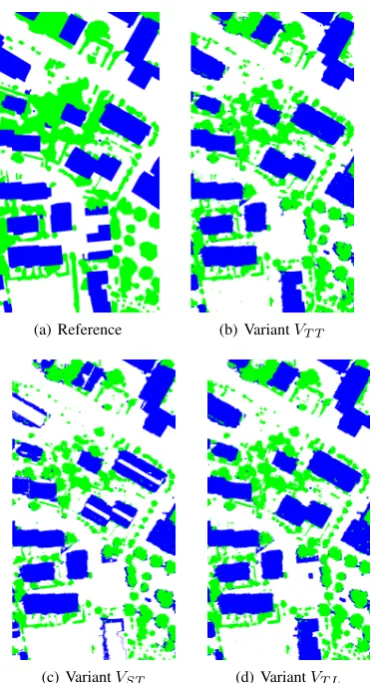
A general evaluation of completeness and correctness per class cannot be given here for lack of space. We present exemplary results for test pair30/34(S/T) in figure 4 and give the corre-sponding quality measures per class in table 1. Both, the figure and the table show that the results after TL (VariantVT L)
corre-spond closely to what can be achieved if training samples from the target domain are used (VariantVT T), while showing a
con-siderable improvement over the variant without transfer (VST).
(a) Orthophoto
nDSM
NDVI
(b) Feature space Figure 3: Orthophoto and feature space for patch 17. Colours:
ground(white),building(blue) andtree(green).
Variant Class OA
[%]
ground build. tree
VT T
Comp.[%] 91.0 90.3 73.6
85.9
Corr.[%] 83.9 89.9 85.9
Quality[%] 77.4 82.0 65.7
VST
Comp.[%] 94.4 78.3 60.7
80.9
Corr.[%] 74.8 87.4 92.0
Quality[%] 71.7 70.3 57.7
VT L
Comp.[%] 92.7 91.2 68.7
85.6
Corr.[%] 82.4 89.5 88.7
Quality[%] 77.3 82.4 63.1
Table 1: Overall accuracy (OA), completeness (Comp.), correct-ness (Corr.) and quality values for the classesground,building (build.) andtree, obtained for the three variants of the test (VT T,
VST,VT L) in pair 30/34 (S/T).
4.3 Parameter sensitivity analysis
The influence of the three most important parameters in terms of TL quality and our proposed instance weighting approach are studied here to show the stability of the proposed methodology. In these experiments, one parameter is varied, whereas all other settings remain constant as described in Section 4.1. We evaluate the averageOAover the 36 tests for the three variants described in the previous sections and additionally include the averageOA achieved by DA in the cases of positive transfer (V+
T L). The
re-sults are presented in figure 5.
The first parameter is the number of samples per class to trans-fer (figure 5(a)). Here we useρE = ρA =ρ, i.e., the number
of source samples to be removed fromT Di is identical to the number of target samples to be added in each iteration. The best average OA ofVT Lwas achieved for our standard setting with
ρ = 30. Larger as well as lower values forρled to poorer av-erage transfer performance. The valueρ= 10even led to nega-tive transfer measured in average OA ofVT Lcompared toVST.
The good result forV+
T Lin case ofρ= 10is not representative
(a) Reference (b) VariantVT T
(c) VariantVST (d) VariantVT L
Figure 4: Reference data and results of classification of the tar-get area for test pair30/34for the three classification variants. Colours:ground(white),building(blue) andtree(green).
and too fast changes caused by removal of certain source samples from and adding semi-labeled target samples to the setT Di.
The second parameter is the number of neighbours forknn anal-ysis and class prediction. The value of neighbours forknn anal-ysis and class prediction for our standard casek = 19seems to be a good choice, this led to slightly worse result in average OA ofVT LandVT L+ than the best case in this study with value
k= 20. The changes of this parameter causes only small differ-ences in average OA ofVT L. It would seem that the choice of
this parameter is not crtitical for the quality of transfer.
The last parameter in our sensitivity analysis is the parameterh of the weight function in equation 10. The best results of average OA of VT Lare achieved byh values between0.50and 0.70,
the best of which corresponds to our standard caseh = 0.70. Somewhat surprisingly, usingh= 0.10also leads to a relatively good result in variantVT L, though the averageOAfor the cases
of positive transfer (V+
T L) is worst in this case. This indicates that
the relatively high totalOA is due to a lower decrease inOA for the cases of negative transfer rather than to an improvement in the cases of positive transfer. The valuesg(pn, h = 0.1) ∈
[0.01..0.99]correspond topn∈[0.03..0.33]. As we have three
classes, the maximum of the posterior will be larger than 1/3, so that for all target samples and for all consistent source samples, such low values forpnwill only occur with inconsistent source
samples in the TL process (cf. Section 3.2.3 and equation 11). This shows that the proper handling of these source samples may have a relatively high influence on the quality of transfer.
All parameter changes during the tests result in quite stable
chang-(a) Dependency on the numberρof samples to transfer.
(b) Dependency on the number of neighbours forknnanalysis and class prediction.
(c) Dependency on the parameterhof the weight function. Figure 5: Dependency of the average overall accuracy (over 36 tests) on different parameter settings.
es of theOAforVT LandVT L+, which confirms the stability and
robustness of our methodology.
5. CONCLUSIONS AND FUTURE WORK
criti-cal cases in which the assumptions about the feature distributions were violated, leading to a negative transfer.
In the future, we will investigate alternative strategies for sam-ple selection and weight definition that might further increase the transfer performance, and we want to investigate the impact of a higher-dimensional feature space. Furthermore, strategies for detecting cases of negative transfer automatically would allow us to fully exploit the benefits of DA. We will test our method on different data sets using a feature space of higher dimension and also differentiating more classes. We will also compare our method to other techniques, e.g. to semi-supervised classification as proposed in (Amini and Gallinari, 2002). Finally, we want to compare our methodology to a setting in which a small amount of labelled samples is available in the target domain.
ACKNOWLEDGEMENTS
This work was supported by the German Science Foundation (DFG) under grant HE 1822/30-1. The Vaihingen data were pro-vided by the German Society for Photogrammetry, Remote Sens-ing and Geoinformation (DGPF) (Cramer, 2010):
http://www.ifp.uni-stuttgart.de/dgpf/DKEP-Allg.html.
References
Abe, S., 2006. Support Vector Machines for Pattern Classifica-tion. 2ndedn, Springer, New York (NY), USA.
Acharya, A., Hruschka, E. R., Ghosh, J. and Acharyya, S., 2011. Transfer learning with cluster ensembles. In: Proceedings of the ICML Workshop on Unsupervised and Transfer Learning, pp. 123–132.
Amini, M.-R. and Gallinari, P., 2002. Semi-supervised logistic regression. In: Proceedings of the 15thEuropean Conference on
Artificial Intelligence, pp. 390–394.
Banerjee, B., Bovolo, F., Bhattacharya, A., Bruzzone, L., Chaud-huri, S. and Buddhiraju, K., 2015. A novel graph-matching-based approach for domain adaptation in classification of remote sens-ing image pair. IEEE Transactions on Geoscience and Remote Sensing 53(7), pp. 4045–4062.
Bishop, C. M., 2006. Pattern Recognition and Machine Learning. 1stedn, Springer, New York (NY), USA.
Bruzzone, L. and Marconcini, M., 2009. Toward the automatic updating of land-cover maps by a domain-adaptation SVM clas-sifier and a circular validation strategy. IEEE Transactions on Geoscience and Remote Sensing 47(4), pp. 1108–1122.
Bruzzone, L. and Prieto, D., 2001. Unsupervised retraining of a maximum likelihood classifier for the analysis of multitemporal remote sensing images. IEEE Transactions on Geoscience and Remote Sensing 39(2), pp. 456–460.
Cauwenberghs, G. and Poggio, T., 2001. Incremental and decre-mental support vector machine learning. In: Advances in Neural Information Processing Systems 13, pp. 409–415.
Cheng, L. and Pan, S. J., 2014. Semi-supervised domain adapta-tion on manifolds. IEEE Transacadapta-tions on Neural Networks and Learning Systems 25(12), pp. 2240–2249.
Cramer, M., 2010. The DGPF test on digital aerial camera evalua-tion – overview and test design. Photogrammetrie Fernerkundung Geoinformation 2(2010), pp. 73–82.
Durbha, S., King, R. and Younan, N., 2011. Evaluating transfer learning approaches for image information mining applications. In: Proceedings of the IEEE International Geoscience and Re-mote Sensing Symposium (IGARSS), pp. 1457–1460.
Gopalan, R., Li, R. and Chellappa, R., 2011. Domain adaptation for object recognition: An unsupervised approach. In: Proceed-ings of the IEEE International Conference on Computer Vision (ICCV), pp. 999–1006.
Klein, H. and F¨orstner, W., 1984. Realization of automatic error detection in the block adjustment program PAT-M43 using robust estimators. International Archives of Photogrammetry and Re-mote Sensing XXV-3a, pp. 234–245.
Kuznetsova, A., Hwang, S. J., Rosenhahn, B. and Sigal, L., 2015. Expanding object detector’s horizon: Incremental learning framework for object detection in videos. In: Proceedings of the IEEE Conference on Computer Vision and Pattern Recognition (CVPR), pp. 28–36.
Pan, S. J. and Yang, Q., 2010. A survey on transfer learning. IEEE Transactions on Knowledge and Data Engineering 22(10), pp. 1345–1359.
Paul, A., Rottensteiner, F. and Heipke, C., 2015. Transfer learn-ing based on logistic regression. International Archives of the Photogrammetry, Remote Sensing and Spatial Information Sci-ences XL-3/W3, pp. 145–152.
Rutzinger, M., Rottensteiner, F. and Pfeifer, N., 2009. A compari-son of evaluation techniques for building extraction from airborne laser scanning. IEEE Journal of Selected Topics in Applied Earth Observations and Remote Sensing 2(1), pp. 11–20.
Sugiyama, M., Krauledat, M. and M¨uller, K.-R., 2007. Covariate shift adaptation by importance weighted cross validation. Journal of Machine Learning Research 8, pp. 985–1005.
Thrun, S. and Pratt, L., 1998. Learning to learn: Introduction and overview. In: S. Thrun and L. Pratt (eds), Learning to Learn, Kluwer Academic Publishers, Boston, MA (USA), pp. 3–17.
Tuia, D., 2014. Weakly supervised alignment of image mani-folds with semantic ties. In: Proceedings of the IEEE Interna-tional Geoscience and Remote Sensing Symposium (IGARSS), pp. 3546–3549.
Tuia, D., Munoz-Mari, J., Gomez-Chova, L. and Malo, J., 2013. Graph matching for adaptation in remote sensing. IEEE Transac-tions on Geoscience and Remote Sensing 51(1), pp. 329–341.
Tuia, D., Volpi, M., Trolliet, M. and Camps-Valls, G., 2014. Semisupervised manifold alignment of multimodal remote sens-ing images. IEEE Transactions on Geoscience and Remote Sens-ing 52(12), pp. 7708–7720.
Vishwanathan, S., Schraudolph, N., Schmidt, M. W. and Murphy, K. P., 2006. Accelerated training of conditional random fields with stochastic gradient methods. In: Proc. 23rd International Conference on Machine Learning (ICML), pp. 969–976.
Wegner, J. D., Rottensteiner, F., Gerke, M. and Sohn, G., 2016. The ISPRS 2D Labelling Challenge. http://www2.isprs.org/commissions/comm3/wg4/semantic-labeling.html. Accessed 11/03/2016.
Zadrozny, B., 2004. Learning and evaluating classifiers under sample selection bias. In: Proceedings of the 21stInternational Conference on Machine Learning, pp. 114–121.

![Figure 2: Overall accuracy [%] for the 36 test pairs, obtained for three classification variants (red: VST ; blue: VT T ; green: VT L)](https://thumb-ap.123doks.com/thumbv2/123dok/3218835.1394991/6.595.62.538.70.208/figure-overall-accuracy-pairs-obtained-classication-variants-green.webp)