ACCURACY ASSESSMENT OF A UAV-BASED LANDSLIDE MONITORING SYSTEM
M. V. Peppa a*, J. P. Mills a, P. Moore a, P. E. Miller b, J. E. Chambers c
a School of Civil Engineering and Geosciences, Newcastle University, Newcastle upon Tyne, UK – (m.v.peppa, jon.mills, philip.moore)@ncl.ac.uk
b The James Hutton Institute, Aberdeen, UK - [email protected] c British Geological Survey, Keyworth Nottingham, UK - [email protected]
Commission V, WG V/5
KEY WORDS: Landslides, UAV, structure-from-motion, georeferencing, bundle adjustment, DEM
ABSTRACT:
Landslides are hazardous events with often disastrous consequences. Monitoring landslides with observations of high spatio-temporal resolution can help mitigate such hazards. Mini unmanned aerial vehicles (UAVs) complemented by structure-from-motion (SfM) photogrammetry and modern per-pixel image matching algorithms can deliver a time-series of landslide elevation models in an automated and inexpensive way. This research investigates the potential of a mini UAV, equipped with a Panasonic Lumix DMC-LX5 compact camera, to provide surface deformations at acceptable levels of accuracy for landslide assessment. The study adopts a self-calibrating bundle adjustment-SfM pipeline using ground control points (GCPs). It evaluates misalignment biases and unresolved systematic errors that are transferred through the SfM process into the derived elevation models. To cross-validate the research outputs, results are compared to benchmark observations obtained by standard surveying techniques. The data is collected with 6 cm ground sample distance (GSD) and is shown to achieve planimetric and vertical accuracy of a few centimetres at independent check points (ICPs). The co-registration error of the generated elevation models is also examined in areas of stable terrain. Through this error assessment, the study estimates that the vertical sensitivity to real terrain change of the tested landslide is equal to 9 cm.
1. INTRODUCTION
1.1 Background
Landslides represent complex and dynamic phenomena that have the potential to impact disastrously on society. Reliable approaches to interpret, monitor and mitigate landslide hazards are therefore crucial. There are various categories of landslides relating to different material types, movement mechanisms and velocities (Cruden and Varnes, 1996). Selecting the most appropriate monitoring approach, and determining the necessary sensitivity for detecting failure is therefore an important consideration.
Traditionally, ground-based geotechnical and geophysical investigations have been used to monitor the internal structure of landslides. However, because most geotechnical techniques provide observations at discrete locations, they yield low spatial resolution (Merritt et al., 2014). Some geophysical methods offer higher resolution, providing transect based observations (e.g. Electrical Resistivity Tomography). However, these methods often provide indirect information (e.g. physical property information) that requires cross-validation from benchmark observations obtained by other techniques (Chambers et al., 2011; Merritt et al., 2014). Airborne laser scanning (ALS) and terrestrial laser scanning (TLS) provide high density point clouds enabling generation of high quality digital elevation models (DEMs) (Ackermann, 1999; Pirotti et al., 2013). Nevertheless, both techniques are relatively costly and, in the case of TLS, occlusions can occur due to oblique incidence angles (Eisenbeiß, 2009). Mini UAVs fitted with off-the-shelf compact cameras have recently become attractive for many photogrammetric applications because they offer time-efficient and cost-effective
* Corresponding author
solutions compared to traditional aerial photogrammetric surveys, thereby enabling capture at high spatio-temporal resolution. Also, the recent development of per-pixel image matching algorithms (e.g. stereo semi-global matching algorithm Hirschmüller (2008)), utilised in SfM approaches (Snavely et al., 2008), facilitate the automatic generation of dense point clouds from overlapping imagery (Remondino et al., 2014). Overall, UAV-derived multi-temporal observations based on a SfM workflow can complement contemporary ground-based investigations and enhance the interpretation of landslide activity.
1.2 Suitability of UAVs for monitoring purposes
Niethammer et al. (2012) monitored a landslide in the French Alps using a mini quad-rotor UAV, equipped with a Praktica Luxmedia digital camera, from approximately 200 m altitude. They generated a DEM of 6 cm GSD using a SfM approach, adequate to identify fine surface fissures of 10 cm width that could not be detected in conventional airborne imagery. In a similar study, d'Oleire-Oltmanns et al. (2012) extracted a DEM of 5 cm resolution using a mini fixed-wing UAV, flying at 85 m altitude with a Panasonic Lumix GF1 digital camera to monitor gully development in Morocco. They achieved a 3D accuracy of a few centimetres at ICPs. Both of these studies illustrated that mini-UAV systems equipped with off-the-shelf compact digital cameras, complemented by the SfM workflow, are capable of delivering DEMs with a resolution and accuracy comparable to TLS for monitoring applications (Eltner et al., 2015).
al., 2014). These errors have been found to originate from various sources such as low overlap, blurry images, flight configuration, number and distribution of GCPs, as well as the various geometric camera models used in the different SfM software. For example, low overlap might yield mismatches during the initial image alignment step of the SfM pipeline and generate discontinuities in the reconstructed dense point cloud. This, in turn, can destabilise the bundle adjustment solution and errors can propagate into the DEMs (Harwin et al., 2015). The higher the image overlap the greater the number of optical rays that intersect an object point, thereby attaining increased redundancy in point determination (Haala and Rothermel, 2012). Blurred images are caused by wind, sudden turbulence and forward motion of the UAV (Sieberth et al., 2014). As Sieberth et al. (2014) noted, image blur deteriorates the image sharpness which might influence the camera calibration results when the automatic SfM pipeline is applied. James and Robson (2014) demonstrated that parallel flight lines can cause vertical systematic errors with a bowl-shape pattern, due to the poor imaging network geometry. According to their analysis, these errors can be significantly reduced when convergent images are acquired or flight lines are flown in opposing directions. The same study also highlighted that evenly distributed GCPs should be included into the bundle adjustment in order to reduce the aforementioned systematic patterns. Furthermore, Eltner and Schneider (2015) investigated Agisoft PhotoScan, a popular commercial SfM software, and demonstrated that the geometric camera model was unable to entirely resolve the lens distortion of a Panasonic Lumix DMC-LX3 camera. This was found to be particularly relevant in the case of low-cost cameras and in the absence of GCPs. The unresolved distortion might form bowl-shape systematic patterns that were recognisable either in the undistorted images (Eltner and Schneider, 2015) or in the vertical error distributions at ICPs (James and Robson, 2014).
Apart from systematic errors in the SfM workflow, other recent studies have investigated noise caused by vegetation (Javernick et al., 2014; Tonkin et al., 2014). Tonkin et al. (2014) reported that the elevation differences between observations obtained with SfM and a total station were higher in areas vegetated with heather than in short grassland. Javernick et al. (2014) identified regions with vegetation height higher than 0.40 m in a SfM-derived DEM. They firstly generated a 0.50 m DEM resolution by calculating the minimum elevation of each pixel. Then, they degraded the original spatial resolution of the SfM-derived dense point cloud, to create different DEMs of coarser resolution and subtracted them from the initial DEM. In this way, they mapped the regions of vegetation noise. However this approach is likely to smooth regions of local surface variations.
In the context of landslide monitoring, it is crucial to account for all error sources in order to reliably estimate the real terrain change. Therefore, the research presented in this paper addresses the aforementioned systematic errors that are propagated into the SfM-derived elevation differences through the self-calibrating bundle adjustment process. In addition, vegetation variations, which also influence elevation differences, are also considered. As a result of the analysis, vertical measurement sensitivity (accuracy) is quantified for a real-world landslide over a monitoring period of two years.
2. SYSTEM CHARACTERISTICS AND STUDY AREA
2.1 UAV system
A Newcastle University-owned mini fixed-wing UAV (Quest UAV 300) was used for all data collection in this project. This
UAV has a maximum payload of 5 kg and a flight duration of approximately 15 minutes utilising a Lithium polymer battery. The UAV platform is equipped with a compact digital camera (as detailed below), an on-board single-frequency Global Navigation Satellite System (GNSS) receiver and a consumer-grade Micro-Electro Mechanical System-Inertial Measurement Unit (MEMS-IMU). It also contains a micro-processor with autopilot software that interprets predefined flight mission parameters (a series of 3D way-points that describe the flight path and the camera exposure time) enabling the UAV to fly autonomously.
The on-board camera is a Panasonic Lumix DMC-LX5 with a 5.1 mm nominal focal length Leica lens for visible image acquisition. The camera has a 1/1.63" (8.07 x 5.56 mm) CCD sensor with 2 x 2μm pixel size, creating an image of 3648 x 2736 pixels. It is mounted on gel, for vibration damping, and fitted in the UAV body. A simple gimbal, attached to the UAV body, compensates for the aircraft's movements along the roll axis enabling the camera to capture nadir images.
2.2 Study area
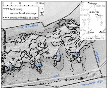
The landslide study area is located at Hollin Hill (54º 6' 38.90'' N, 0º 57' 36.84'' W), North Yorkshire, UK (Figure 1), and is a British Geological Survey (BGS) landslide observatory site. The site occupies farmland used for rough grazing and is mainly vegetated with short grass, and occasional trees and shrubs. The study area extends approximately 290 m E-W and 230 m N-S. It has an average slope of 12º and a 50 m elevation difference from N-S.
Figure 1. Geomorphological map of Hollin Hill landslide. Inset map locates the site within the UK (Merritt et al., 2014).
Chambers et al. (2011) characterised the Hollin Hill landslide as a very slow moving multiple earth slide-earth flow with an average displacement rate of 2 m/yr. Investigations by the BGS identified shallow rotational movements of weak materials at the upper parts of the slope and translational movements at the lower parts of the slope. Many scarps and cracks have emerged at the top, while the sliding material towards the bottom of the slope has formed four pro-grading lobes, as illustrated in Figure 1.
subsurface movements have been monitored by BGS with multiple geophysical, geotechnical and ground-based RTK-GNSS observations (Chambers et al., 2011; Gunn et al., 2013). This active landslide provides an ideal study area to investigate the potential of the UAV approach for assessing multi-temporal landslide deformations.
3. METHODOLOGY AND DATA ANALYSIS
3.1 Fieldwork and image acquisition
Six field campaigns were carried out spanning a period of almost two years, as listed in Table 1. During the fieldwork the following tasks were performed: (1) GNSS base station was established on stable terrain in an adjacent field and observed in GNSS static mode for at least six hours, which delivered 1 cm planimetric and 2 cm vertical absolute accuracy; (2) circular targets of 0.40 m diameter were evenly distributed over the landslide and were surveyed in GNSS rapid static mode (three-minute observations), which delivered 3D accuracy at mm-level relative to the GNSS base station; (3) visible UAV imagery was collected at the specification described below; and (4) spot heights of characteristic concave/convex landslide features were topographically surveyed using total station and/or rapid static GNSS for validation purposes. Due to time limitations, topographic surveying in (4) was only performed at four epochs, in December 2014, March 2015, June 2015 and February 2016.
The flight configuration and error statistics, as calculated in PhotoScan, are reported in Table 1 for the six epochs.
Ca field campaigns at the Hollin Hill landslide.
For the first three campaigns listed in Table 1, the camera was set in shutter priority mode with a shutter speed of 1/800 s, at ISO 400 and varying aperture. An exposure interval of 2.5 seconds enabled image capture with a standard 60% fore/aft and 40% lateral overlap, assuming a constant UAV speed of 20 m/s. After gaining a better understanding of the UAV’s operational capabilities under different wind conditions, the settings for the last three campaigns were changed. In particular, the exposure interval was set to 2 seconds and the lateral overlap increased to 70% to enable better overlapping coverage. The camera was set up with a fixed shutter speed of 1/800 s to decrease image blurring, ISO 100 to ensure that images were captured with low noise (Sieberth et al., 2014) and a fixed aperture of f/2 to ensure that sufficient light reached the sensor. Further, in the final three campaigns, flight lines in opposing directions were also added, according to the recommendations of James and Robson (2014), in order to achieve a better flight configuration and minimise systematic errors.
3.2 DEM generation and elevation difference determination
3.2.1 Image alignment: Firstly, blurred and oblique images
were manually excluded from processing. Corresponding points were detected across the remaining images to enable multiple stereo-pair reconstruction. Bundle adjustment solved for (a) the interior orientation camera parameters (IOP), i.e. focal length, sensor size, radial and tangential distortion coefficients for the entire photogrammetric block, and (b) the relative orientation and translation of each image (Eltner and Schneider, 2015; Remondino et al., 2014). The image alignment step was undertaken in Agisoft PhotoScan (version 1.2.3) (PhotoScan, 2016).
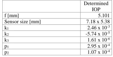
Typically, in PhotoScan, an initial value for the focal length is automatically extracted from the exchangeable image file format (EXIF) information of the acquired images. For this study, a separate indoor calibration was performed in September 2015 prior to that month’s flight. An indoor calibration test field was established using calibration targets at several depths over a 6 m range, the positions of which were precisely surveyed using a total station. Three images at 0º and ±90º roll angles were captured from four different positions. The camera calibration was performed in PhotoScan and the determined parameters are shown in Table 2. The indoor calibration provided approximate values for the camera's IOP that were more relevant than the values extracted from the EXIF information. These values were then refined through self-calibration in the SfM pipeline.
Determined
Table 2. Parameters of indoor camera calibration.
3.2.2 Georeferencing: GCPs were utilised to scale and
orientate the corresponding points (tie points) into a fixed reference frame (Ordnance Survey Great Britain 1936 (OSGB36)) in PhotoScan. The GCPs were used as external constraints, in combination with the inner constraints (i.e. detected corresponding points), thereby allowing the self-calibrating bundle adjustment to converge to a stable solution that minimises the reprojection errors (Nex and Remondino, 2014). These quantify the pixel differences between the initially detected corresponding points and those estimated and back-projected into the images through the SfM pipeline (Haala and Rothermel, 2012). Corresponding points with reprojection errors greater than 1.5 pixels were automatically removed to optimise the solution. Image alignment and georeferencing resulted in sub-pixel mean reprojection errors for all epochs, as summarised in Table 1.
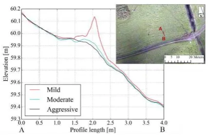
correspondent disparity, by recursively assigning costs based on pixel value differences of its nearest neighbours (Remondino et al., 2014). The matched pixels are then triangulated to form the resulting 3D dense point cloud. The assigned cost serves as a smoothing filter for the surface representation. PhotoScan offers different filtering options such as mild, moderate and aggressive. According to the PhotoScan instruction manual, the mild option maintains minor surface details, the aggressive option filters out these details and the moderate option offers an intermediate smoothing result. Figure 2 illustrates a section through a reconstructed dense point cloud located across a shrub with height lower than 0.50 m. The aggressive filter option was adopted because it was seen (as evidenced in Figure 2) to remove points from such low vegetated areas. However, points that represented higher vegetation and various objects (such as monitoring sensors, fences, sheep, people and cars) were not entirely filtered out. Consequently, the ground classification algorithm in TerraSolid TerraScan (TerraScan, 2016) was also utilised to further clean the reconstructed dense point cloud.
Figure 2. Profile of a dense point cloud reconstructed with three different filtering options; mild, moderate and aggressive. Inset orthoimage locates the profile within the study area.
3.2.4. Interpolation and elevation difference
determination: The cleaned dense point cloud was imported to the Orientation and Processing of Airborne Laser Scanning data (OPALS) software (Pfeifer et al., 2014), to generate a raster elevation model. This used the moving planes approach, which fits the best tilted plane to 15 nearest neighbouring points, by minimising the vertical distance in a least-squares sense. In this manner, the elevation of a grid point with a 6 cm spatial resolution was calculated. This interpolation technique was adopted because it best accounts for the relatively extreme local surface variations. Also, the 6 cm DEM resolution was calculated at approximately 2xGSD (see Table 1) to ensure that a continuous surface without pixel voids could be generated for all epochs. Each DEM-epoch was subsequently subtracted from the February 2016 DEM on a pixel-by pixel basis in order to determine elevation differences.
3.3 Accuracy assessment and vertical sensitivity
It is important to check the stability of the self-calibrating bundle adjustment solution across epochs. To achieve this, radial distortion curves were computed for all epochs using the Brown (1971) model. The curves were derived using the adjusted distortion coefficients determined through the SfM pipeline. The distortion curves were compared to one another and also against the distortion curve derived from the indoor calibration.
After computing the DEM differences as described in Section 3.2.4, errors from various sources (as described in Section 1) may
mask real topographic change. An accuracy assessment was performed to determine how these errors influenced the outputs. PhotoScan was used to compute residuals at all ICPs, which expresses the differences in coordinates between GNSS-surveyed and SfM derived positions. The planimetric vectors at ICPs were also calculated. For May 2014, December 2014 and March 2015 epochs the RMSEs were calculated for both GCPs and ICPs due to the limited number of available ICPs. Furthermore, to ensure that the generated DEMs were correctly registered vertically with each other, the elevations of the interpolated grid points within areas of stable and flat terrain were compared for each epoch against the February 2016 DEM. A 162 m2 area was extracted from the vehicle track near the toe of the slope where only bare ground exists (see Figure 1). The elevations of the interpolated grid points from this area were extracted from the SfM-derived DEMs. The elevation differences per pair, in terms of the mean, standard deviation and RMSE statistics, were calculated using Cloud Compare (CloudCompare, 2016).
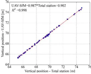
The vertical accuracy was also assessed for each epoch using an independent set of observations. These observations were obtained using GNSS and total station instruments to measure spot heights. Vertical coordinates for each XY spot height location were extracted from the generated DEMs through bilinear interpolation of adjacent cells. Least-squares linear regression was applied to inspect the relationship between the observed and estimated elevations at the spot heights.
The vertical sensitivity indicates the threshold of detectable elevation change that is possible given the adopted methodology and associated errors propagated into the generated DEMs. In order to derive the threshold, a classical error propagation approach was applied to the elevation differences (Wolf and Ghilani, 1997) and a 99% confidence level applied, as described in Equation 1.
�� ���� �� � ��� � = √�����+ ������� 6 (1)
where t = 2.96, critical value for 99% confidence level;
σDEMi is the standard deviation of DEM at epoch i;
σDEMFeb16 is the standard deviation of February 2016 DEM.
The standard deviations for DEMs at each epoch were computed in OPALS. The moving planes approach allowed the calculation of standard deviation for each grid point of the SfM-derived DEM, according to the residuals of the best fit plane through the neighbouring points. The error propagation was then applied for each grid point and the standard deviation of each elevation difference was computed creating one raster per pair. The maximum value of this raster was chosen as the standard deviation of the elevation differences between two epochs.
4. RESULTS AND DISCUSSION
4.1 Adjusted calibration
The May 2014 and December 2014 curves produced the highest difference (approximately 11 μm) to the Feb 2016 reference curve at the outer corners of the image. This corresponds to 5.5 pixels or 33 cm ground distance for a DEM of 6 cm resolution. The May 2014 curve starts to deviate from the reference with approximately 1 pixel difference, at a radial distance smaller than 2 mm.
Figure 3. Radial distortion curves. The grey zone indicates the confidence level of ± 3σ.
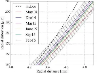
Even though the same software was used for both indoor and in-flight calibration, the radial distortion curves for all epochs significantly deviate from the indoor radial distortion curve after 4.3 mm radial distance (Figure 4). This is mainly because the indoor calibration was carried out under a different scenario with different camera settings.
Figure 4. Detail of the radial distortion curves at the outer corner of the image.
As a result of this assessment, there is clear evidence that for the first three campaigns (all performed for imaging networks with low percentage overlap) the distortion curves deviate more from the reference than for the remaining curves of flights with a better overlapping network of images. Apart from the different imaging networks, the different camera settings (as described in Section 3.1) also influences these results.
4.2 Planimetric and vertical error assessment
Planimetric and vertical RMSEs per epoch, shown in Table 1, vary from 1.2 cm to 3.8 cm. The vertical RMSEs were interpolated with a bi-cubic interpolation to form a continuous error surface, as illustrated in Figure 5. This shows the vertical error distribution across the study area. It is expected that the error should be close to zero creating a randomly distributed pattern of errors. Due to the different error sources mentioned in Section 1, vertical errors were observed particularly for the first
campaign (see Figure 5a), most notably over regions of low overlap in the north-east corner of the site. For the remaining campaigns the magnitude of the vertical error was relatively small by comparison, although June 2015 (Figure 5d) displayed higher errors across the north of the site. This is likely to have originated from strong gusts of wind which destabilised the UAV while it was turning from east to south creating blurred images over that region. As mentioned in Section 1, the use of such blurred images might yield vertical deformations (James and Robson, 2014; Sieberth et al., 2014).
Planimetric error vectors at ICPs are also included in Figure 5. As illustrated, no general systematic directional pattern was observed at ICPs. This indicates that a reliable solution was achieved in the horizontal plane for all epochs. There are, however, a few planimetric vectors of comparatively higher magnitude, for example an 8.8 cm planimetric error in September 2015 at ICP 6 (Figure 5e). This error might have originated from a few blurred images acquired over that region which degraded the image resolution (Sieberth et al., 2014). Even though the extremely blurred images were excluded at the beginning of the workflow, a few still remained and could not be removed as this would have resulted in insufficient overlapping images. There is also an 11.5 cm planimetric error in May 2014 at ICP 9 (Figure 5a). This ICP is visible only from two images due to poor imaging network over that region. The position of ICP 9 was estimated with low redundancy and this caused the high planimetric error.
To alleviate bowl-shape deformations, James and Robson (2014) recommended improvements to the imaging network by including convergent-off-nadir imagery and utilising overlapping flight strips flown in opposing directions. In this study, the first recommendation cannot be applied because of the fixed-wing UAV design – unlike multi-rotor platforms the camera pointing direction cannot be adjusted to collect oblique imagery. However, by including flight strips in opposing directions, it was possible to externally control the bundle adjustment with only five GCPs and still produce DEMs with relatively low vertical deformations, as evidenced by the final three campaigns (Figure 5d, 5e and 5f).
4.3 Co-registration evaluation and cross-validation
Statistical measures of elevation differences over stable terrain, (the vehicle track) are described in Table 3.
Epoch pair
Mean difference
[cm]
Standard Deviation
[cm]
RMSE [cm]
February 2016-May 2014 4.6 3.0 5.5
February 2016-December 2014 2.7 2.1 3.4 February 2016-March 2015 2.8 1.2 3.0 February 2016-June 2015 5.4 1.8 5.7 February 2016-September 2015 3.6 1.4 3.8
Table 3. Statistical measures to evaluate DEM pair co-registration over 162 m2 area of stable terrain.
Figure 5. Planimetric and vertical RMSE errors at ICPs in (a) May 2014, (b) December 2014, (c) March 2015, (d) June 2015, (e) September 2015 and (f) February 2016 campaigns. For (a), (b) and (c) the errors are calculated for both GCPs and ICPs due to a relatively limited number of ICPs (see Table 1).
RMSE vertical errors in the range of 10 to 13 cm were achieved, which is approximately double the GSD. The statistical values of the first two campaigns were slightly poorer than the final two. This is most likely due to inferior image network configurations.
Campaign
Number of points
Mean [cm]
Standard Deviation
[cm]
RMSE [cm]
December 2014 48 4.7 10.0 11.0
March 2015 52 -11.1 7.9 13.1
June 2015 98 -5.0 9.0 10.2
February 2016 65 5.8 8.7 10.4
Table 4. Comparison of the SfM derived elevations against independently observed elevations at sample points.
The regression analysis (Figure 6) demonstrated that there were no major outliers present, and no systematic offset between the reference and SfM validation observations for the February 2016 campaign. The analysis of the three remaining campaigns also provided a similar pattern, with close to 1:1 linear relationship.
Figure 6. Regression analysis between SfM derived and observed elevations at validation points for Feb16 image acquisition.
4.4 Vertical sensitivity and elevation differences
The vertical sensitivity was calculated using Equation (1) for each elevation difference pair. The standard deviation for all pairs varied between ± 0.1 cm and ± 3.0 cm. By applying the 99% confidence level, the maximum value of vertical sensitivity is ± 9.0 cm. As a result, elevation changes less than ± 9.0 cm cannot be assumed to represent real surface deformations, being below the noise level of co-registration and other errors, as discussed throughout the paper.
The elevation differences per pair are illustrated in Figure 7. The eastern and western lobes, as well as the back scarp, constitute the most active parts of the landslide, as depicted in Figure 8b. The surface changes occurred predominantly along the convex and concave geomorphological features (see Figures 1 and 7 for comparison). Part of the western lobe has collapsed (24m2 in extent), sliding downwards, and created a dramatic change of -0.70 m maximum ground loss and a + 0.50 m maximum ground accumulation within the last two years. The failure appears to have occurred between the September 2015 and February 2016 epochs. As far as the eastern lobe is concerned, ground material has continuously accumulated at the toe of the eastern lobe, which appears to have surged forward post-May 2014. Here, the maximum observed positive elevation change was + 0.70 m, between February 2016 and May 2014. Over the duration of the final three campaigns the surface of the eastern lobe’s toe has not significantly changed compared to other epochs. At the back scarp a maximum ground subsidence of approximately - 0.20 m was observed at the top of the slope, whereas material sliding down-slope created a maximum elevation increase of approximately + 0.30 m over the observation period.
Figure 7. Elevation differences between epoch pairs; (a) February 2016-May 2014, (b) February 2016-December 2014, (c) February 2016-March 2015, (d) February 2016-June 2015, (e) February 2016-September 2015. The orthomosaic of the February 2016 epoch, constructed in PhotoScan, is displayed as the background.
Grass growth in May 2014 and September 2015 are observed as negative change in Figures 7a and 7e.
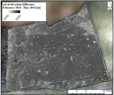
Apart from vegetation differences, there are also other artefacts apparent in the results. For instance, in Figure 7a sudden elevation differences forming linear artefacts were observed in the north-east of the site. These linear artefacts can also be seen in Figure 8, which illustrates the standard deviation of the elevation differences for the February 2016-May 2014 pair. Such artefacts originated from sharp discontinuities that occurred in the generated point cloud due to mismatches (see Section 1). Harwin et al. (2015) explained that it is difficult to remove such discontinuities, especially in grassy terrain, as a photogrammetric approach records the vegetation surface, and is unable to capture underlying terrain, as in the case for ALS for example.
Figure 8. Standard deviation of the elevation differences for the February 2016 – May 2014 pair.
5. CONCLUSIONS AND FUTURE WORK
This paper has presented an investigation of errors associated with SfM-derived elevation differences generated through a UAV landslide monitoring approach. The analysis includes the estimation of the vertical sensitivity by applying the law of error propagation to the generated elevation differences.
Results have shown that RMSE vertical accuracies of approximately 10 cm can be achieved with the use of GCPs and highly overlapping imagery, when SfM-derived elevations are compared against independently observed elevations at sample points. Even though GCPs have been utilised, the derived-DEMs have been shown to still contain vertical systematic errors, due to low overlap flight configurations. When opposing flight strips were added these errors were significantly reduced. The standard deviation of the elevation differences has been shown to provide additional context for error assessment, since this allows spatial illustration of misalignment biases propagated through the processing chain (i.e. Figure 8). Seasonal vegetation changes can, unfortunately, become an obstacle in landslide monitoring, as vegetation cannot be entirely filtered out from the dense point cloud. This research derived a value of ± 9 cm vertical sensitivity for the SfM-derived change measurement, and this appears appropriate for the Hollin Hill landslide site, since the most active parts of the landslide exceeds ± 9 cm elevation change over the revisit period.
measures in combination with the scale-invariant feature transform (SIFT) algorithm.
ACKNOWLEDGEMENTS
This research was 50% funded by a Natural Environment Research Council (NERC) BGS BUFI award (S241) and 50% by a Newcastle University, Engineering and Physical Sciences Research Council (EPSRC) DTA award (EP/L504828/1). The authors wish to thank BGS for providing the geomorphological mapping data and the ALS DEM. The authors would also like to convey their gratitude to the owners of Hollin Hill farm for allowing access to their property. Finally, many thanks to Martin Robertson, Elias Berra, Magdalena Smigaj and Ben Grayson, all of Newcastle University, for assistance during the fieldwork.
REFERENCES
Ackermann, F., 1999. Airborne laser scanning - Present status and future expectations. ISPRS Journal of Photogrammetry and Remote Sensing, 54(2-3), pp. 64-67.
Brown, D.C., 1971. Close-range camera calibration. Photogrammetric Engineering, 37(8), pp. 855-866.
Chambers, J.E., Wilkinson, P.B., Kuras, O., Ford, J.R., Gunn, D.A., Meldrum, P.I., Pennington, C.V.L., Weller, A.L., Hobbs, P.R.N., Ogilvy, R.D., 2011. Three-dimensional geophysical anatomy of an active landslide in Lias Group mudrocks, Cleveland Basin, UK. Geomorphology, 125(4), pp. 472-484.
CloudCompare, 2016. Stand-alone software (http://www.danielgm.net/cc/).
Cruden, D.M., Varnes, D.J., 1996. Landslide types and processes, In: Turner AK, S.R. (Ed.), Landslides, investigation and mitigation. Washington, DC, pp. 36-75.
d'Oleire-Oltmanns, S., Marzolff, I., Peter, K.D., Ries, J.B., 2012. Unmanned Aerial Vehicle (UAV) for monitoring soil erosion in Morocco. Remote Sensing, 4(12), pp. 3390-3416.
Eisenbeiß, H., 2009. "UAV photogrammetry", Institute of Geodesy and Photogrammetry. Swiss Federal Institute of Technology (ETH), Zurich, p. 203.
Eltner, A., Baumgart, P., Maas, H.G., Faust, D., 2015. Multi-temporal UAV data for automatic measurement of rill and interrill erosion on loess soil. Earth Surface Processes and Landforms, 40(6), pp. 741-755.
Eltner, A., Schneider, D., 2015. Analysis of different methods for 3D reconstruction of natural surfaces from parallel-axes UAV images. Photogrammetric Record, 30(151), pp. 279-299.
Gunn, D.A., Chambers, J.E., Hobbs, P.R.N., Ford, J.R., Wilkinson, P.B., Jenkins, G.O., Merritt, A., 2013. Rapid observations to guide the design of systems for long-term monitoring of a complex landslide in the Upper Lias clays of North Yorkshire, UK. Quarterly Journal of Engineering Geology and Hydrogeology, 46(3), pp. 323-336.
Haala, N., Rothermel, M., 2012. Dense multi-stereo matching for high quality Digital Elevation Models. Photogrammetrie, Fernerkundung, Geoinformation, 2012(4), pp. 331-343.
Harwin, S., Lucieer, A., Osborn, J., 2015. The impact of the calibration method on the accuracy of point clouds derived using unmanned aerial vehicle multi-view stereopsis. Remote Sensing, 7(9), pp. 11933-11953.
Hirschmüller, H., 2008. Stereo processing by semiglobal matching and mutual information. IEEE Transactions on Pattern Analysis and Machine Intelligence, 30(2), pp. 328-341.
James, M.R., Robson, S., 2014. Mitigating systematic error in topographic models derived from UAV and ground-based image networks. Earth Surface Processes and Landforms, 39(10), pp. 1413-1420.
Javernick, L., Brasington, J., Caruso, B., 2014. Modeling the topography of shallow braided rivers using Structure-from-Motion photogrammetry. Geomorphology, 213, pp. 166-182.
Merritt, A.J., Chambers, J.E., Murphy, W., Wilkinson, P.B., West, L.J., Gunn, D.A., Meldrum, P.I., Kirkham, M., Dixon, N., 2014. 3D ground model development for an active landslide in Lias mudrocks using geophysical, remote sensing and geotechnical methods. Landslides, 11(4), pp. 537-550.
Nex, F., Remondino, F., 2014. UAV for 3D mapping applications: A review. Applied Geomatics, 6(1), pp. 1-15.
Niethammer, U., James, M.R., Rothmund, S., Travelletti, J., Joswig, M., 2012. UAV-based remote sensing of the Super-Sauze landslide: Evaluation and results. Engineering Geology, 128, pp. 2-11.
Pfeifer, N., Mandlburger, G., Otepka, J., Karel, W., 2014. OPALS - A framework for Airborne Laser Scanning data analysis. Computers, Environment and Urban Systems, 45, pp. 125-136.
PhotoScan, 2016. Stand-alone software (http://www.agisoft.com/). Agisoft LLC
Pirotti, F., Guarnieri, A., Vettore, A., 2013. State of the art of ground and aerial laser scanning technologies for High-resolution topography of the Earth Surface. European Journal of Remote Sensing, 46(1), pp. 66-78.
Remondino, F., Spera, M.G., Nocerino, E., Menna, F., Nex, F., 2014. State of the art in high density image matching. The Photogrammetric Record, 29(146), pp. 144-166.
Sieberth, T., Wackrow, R., Chandler, J.H., 2014. Motion blur disturbs - the influence of motion-blurred images in photogrammetry. Photogrammetric Record, 29(148), pp. 434-453.
Snavely, N., Seitz, S.M., Szeliski, R., 2008. Modeling the world from Internet photo collections. International Journal of Computer Vision, 80(2), pp. 189-210.
TerraScan, 2016. Stand-alone software (http://www.terrasolid.com/products/terrascanpage.php).
Tonkin, T.N., Midgley, N.G., Graham, D.J., Labadz, J.C., 2014. The potential of small unmanned aircraft systems and structure-from-motion for topographic surveys: A test of emerging integrated approaches at Cwm Idwal, North Wales. Geomorphology, 226, pp. 35-43.
Turner, D., Lucieer, A., de Jong, S.M., 2015. Time series analysis of landslide dynamics using an Unmanned Aerial Vehicle (UAV). Remote Sensing, 7(2), pp. 1736-1757.