GEOSTATISTICAL ANALYSIS OF SURFACE TEMPERATURE AND IN-SITU SOIL
MOISTURE USING LST TIME-SERIES FROM MODIS
M. Sohrabinia∗1, W. Rack2and P Zawar-Reza1
1Department of Geography, Atmospheric Research Centre
2Gateway Antarctica, Centre for Antarctic Studies & Research
University of Canterbury Christchurch, New Zealand
[email protected], [email protected], [email protected] http://www.canterbury.ac.nz/
Commission VII/1
KEY WORDS:MODIS, MODIS LST, skin temperature, near-surface soil moisture, land cover, geostatistics, time-series
ABSTRACT:
The objective of this analysis is to provide a quantitative estimate of the fluctuations of land surface temperature (LST) with varying near surface soil moisture (SM) on different land-cover (LC) types. The study area is located in the Canterbury Plains in the South Island of New Zealand. Time series of LST from the MODerate resolution Imaging Spectro-radiometer (MODIS) have been analysed statistically to study the relationship between the surface skin temperature and near-surface SM. In-situ measurements of the skin temperature and surface SM with a quasi-experimental design over multiple LC types are used for validation. Correlations between MODIS LST and in-situ SM, as well as in-situ surface temperature and SM are calculated. The in-situ measurements and MODIS data
are collected from various LC types. Pearson’srcorrelation coefficient and linear regression are used to fit the MODIS LST and surface
skin temperature with near-surface SM. There was no significant correlation between time-series of MODIS LST and near-surface SM from the initial analysis, however, careful analysis of the data showed significant correlation between the two parameters. Night-time series of the in-situ surface temperature and SM from a 12 hour period over Irrigated-Crop, Mixed-Grass, Forest, Barren and Open-Grass showed inverse correlations of -0.47, -0.68, -0.74, -0.88 and -0.93, respectively. These results indicated that the relationship between near-surface SM and LST in short-terms (12 to 24 hours) is strong, however, remotely sensed LST with higher temporal resolution is required to establish this relationship in such time-scales. This method can be used to study near-surface SM using more frequent LST observations from a geostationary satellite over the study area.
1 INTRODUCTION
Near surface soil moisture (SM), defined as the water content of
the upper 10 cm of the soil (Wang and Qu, 2009), is measured by
remote sensing satellites using the electromagnetic radiation in three distinct ranges: the visible and near-infrared region, thermal region and the microwave region. Image analysis and
interpreta-tion techniques such as soil wetness indexes, directly (Bhagat,
2009) or indirectly (Sørensen et al., 2005,Grabs et al., 2009) us-ing remotely sensed data in the visible and near-infrared region are applied to estimate wetness of the near-surface soil layer. The algorithms used in the thermal region are based on the surface energy balance. These algorithms are based on the partition-ing of the net surface energy to the sensible, latent and ground heat fluxes. With the knowledge on the sensible and ground heat
fluxes (QHandQG), which is based on the land surface
temper-ature (LST) and the ancillary data about the surface types under
consideration, the latent heat flux (QE) is estimated (see Eq.1
and 2).QEis used as an indicator of the amount of water
con-tent in the near surface soil layer. Microwave remote sensing techniques in SM analysis rely on known dielectric properties of
the soil and water (Jackson et al., 1996). The advantage of
mi-crowave sensors is the availability of the observations in almost all-weather conditions, which enables more frequent data acquisi-tion; however, compared to the moderate resolution thermal sen-sors, the spatial resolution of these sensors is coarse (Hain et al.,
2011). Other works have used a combination of optical, thermal
and microwave remote sensing data (Wang et al., 2004,Hassan
et al., 2007,Gruhier et al., 2010,Hain et al., 2011). More com-plex methods such as the Soil-Vegetation-Atmosphere-Transfer
(SVAT) model (Carlson et al., 1994) exploit combination of the
remotely sensed data to establish a relationship between surface SM, surface temperature and vegetation cover. Considering the objective of the current research, thermal remote sensing algo-rithms are of interest in this paper.
LST product is one of many datasets derived from day and night observations of the Moderate Resolution Imaging Spectroradiome-ter (MODIS) twin sensors on-board Terra and Aqua satellites, which is a wealth of data covering most of the land masses of the globe over the last 10 years. With a more frequent overpass than Landsat (near-daily) and higher spatial resolution (250, 500 and 1000 m) than some of its predecessors such as the Advanced Very High Resolution Radiometer (AVHRR), MODIS provides a comprehensive series of land, ocean, and atmosphere
obser-vations (LPDAAC, 2010). The LST product is suitable for use
in a variety of research including soil and water resources, agri-culture, climate and atmospheric modelling and research. Infor-mation on LST is necessary for parameterization of land surface
processes in numerical models (Sun and Pinker, 2004). LST is
dependent on the incoming shortwave and longwave radiation, but also landcover (LC) type and the amount of near surface SM. Surface SM affects diurnal change of surface temperature, and it is a key variable in computing several parameters of the land
en-ergy and water budget (Zhang et al., 2007). LST is used for SM
assessment using rigorous physical models, such as Surface En-ergy Balance Algorithm for Land (SEBAL), which estimates SM
based on parameterization of surface heat fluxes (Bastiaanssen,
2000). MODIS LST product archived for more than 10 years is a
issue with these models, however, is the complexity and the risk of compromise in accuracy if good quality data for all the impor-tant parameters in the model are not available. To overcome this issue, an assessment of the relationship between the near surface SM and LST can help to understand the complexity of these two parameters over various LC types in a particular region. Such a relationship can be helpful for approximation of one parameter (SM or LST) with the availability of the other.
This paper is aimed to analyse the correlation between LST using MODIS product with the measured near-surface SM based on geostatistical methods. Daily rainfall data is used to detect the interfering effects of a sudden rainfall on the surface SM, and to discover the time-scale for the best correlation with LST.
2 DATA AND STUDY AREA
2.1 Data
Two distinct datasets, one from the remotely sensed MODIS LST and the second from the in-situ SM measurements provide the inputs for this analysis. The LST product is a scientific dataset derived from MODIS morning and afternoon thermal observa-tions on-board Terra and Aqua satellites. Since the observaobserva-tions in thermal bands of the sensor are also available at night, the prod-uct contain night-time values for evening and midnight, which are collected upon the overpasses of Terra and Aqua satellites on the night side of the planet. The product is derived from bands 31 & 32 (spectral range 10.78-11.28µm & 11.77-12.27µm range, re-spectively). Theoretical background and technical details of the algorithms and procedure for the extraction of LST from MODIS thermal bands is available in the literature (Wan and Dozier, 1996,
Wan, 1999,Wan et al., 2004,Wan, 2008). The dataset is available in hierarchical data format (HDF) and can be accessed online via
Reverbtool.
The in-situ near-surface (<5 cm depth) SM data used in this
paper have been collected in five sites with various land-cover
types. These data have been recorded usingMadgeTechR
digital
soil volumetric moisture data loggers known asSMR110R
. Fre-quency rate of the logged data had been set to every 30 minute. These measurements have been collected from 1st October 2011 till 7th January 2012, however, for consistency with the other datasets only Nov. and Dec. data are used in the analysis.
2.2 Study Area
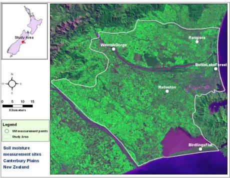
The study area is located in Canterbury Plains in South Island
of New Zealand (Fig.1), at approximate geographic coordinates
43.54 S and 172.31 E in the central point. The in-situ sites were selected in the area for the measurement of the near-surface SM. Criteria for selection of the measurement sites included the area percentage of the dominant LC types, accessibility of the site and finally, a minimum of 1x1 km homogeneous extent of the dom-inant LC type in the area so that at least one pixel from that LC type to be distinguished in the LST satellite dataset.
3 METHODS
3.1 Empirical relationship between near-surface SM and LST
The principle assumption in derivation of SM from LST data in physical models used in thermal remote sensing of SM, such as SEBAL, is partitioning of surface energy to latent and sensible
heat fluxes (Eq.1and 2), and to relate the latent heat to the
amount of moisture content in the near-surface layer. LST from
Figure 1: In-situ soil moisture measurement points overlaid on Landsat image (TM5, 28 March 2011)
the thermal remote sensing observations is accounted for the sen-sible heat part of the energy balance in these models. However, time-lag between the maximum LST on the surface and the
max-imum solar insolation (Wang and Qu, 2009) can also be related
to the amount of surface SM which contribute to the escaping of heat from the surface via latent heat. Without allocation of the
heat energy to theQEby the near-surface SM, the two maxima
(maximum solar insolation and maximum LST) would coincide or be closer in time. To assess this hypothesis, statistical analy-sis of the relationship between the measured surface SM and the remotely sensed LST is implemented in this paper.
Q∗=QG+QE+QH (1)
whereQ∗
is the net radiation,QGis the ground or storage heat
flux,QEis the turbulent latent heat flux, andQHis the
convec-tive sensible heat flux (Rigo and Parlow, 2005,Rigo and Parlow,
2007). Based on Eq.1,QEcan be calculated as:
QE=Q∗−QG−QH (2)
3.2 Land-cover analysis
To identify dominant land-cover classes in the study area, un-supervised classification method has been used. Iterative clas-sification process was carried out using a Landsat TM-5 image acquired on 28 March 2011 over the study area. Eight dominant LC classes were extracted in the region. With the order of high-est to the lowhigh-est percentage these classes included grass, water, irrigated crop/grass, bush, baresoil/fallow, water, fallow/exposed soil, and forest. The in-situ sites were chosen only on five LC classes due to the issues in finding suitable sites for some of the LC types (Table1).
3.3 Construction of LST Time-series
Inside LST scientific datasets (SDSs) derived from MODIS-Terra and MODIS-Aqua, data for each day or night are stored in sepa-rate data fields. To extract correlations between the in-situ SM data and LST from MODIS, time-series of LST product were constructed. Regarding the number of datasets involved in the analysis, reading day and night values for every day during the
analysis period was a cumbersome task, therefore, MatlabR
Sitename LC type Description
Birdlings Flat Open grass non-irrigated seasonal
grassland
Bottlelake Forest dense forest with
spo-radic logged patches
Rangiora Irrigated crop crop under continuous
irrigation
Rolleston Mixed grass grass mixed with tree,
periodic irrigation
Waimak Gorge Barren bare soil in the
Waimakariri river
basin
Table 1: In-situ measurement sites and their LC types
each of the sites. These codes are meant to read data from the entire list of LST HDF files for the analysis period based on the coordinates of each test-site and arrange data-fields alongside the related fields (i.e., LST for day and night fields, quality control field, view-angle and overpass-time fields). Afterwards, dates based on HDF filenames and overpass-time field from the LST SDSs were used in the code to produce sequentially ordered val-ues as time-series from each test-site. It should be mentioned that these time-series are restricted to the available MODIS ob-servations (four times daily in ideal conditions), which is further restricted to those times when cloudless data were available. An-other code was written to match dates and times from LST time-series with the in-situ SM data; this code appends matching data, alongside with the in-situ SM date-time, as extra columns in the time-series of each test-site.
3.4 Statistical methods
Pearson’srcoefficient of correlation (Eq.3) is used to calculate correlations between LST and SM in this paper. Besides
Pear-son’sr, squared form of r indicated asR2 is usually used in
regression analysis, which is known as the regression coefficient of determination. In this paperR2is used alongsiderin order to
provide an absolute measure of agreement between the two vari-ables under consideration. It must be clarified thatR2as used in
regression analysis is more common when prediction of one vari-able based on regressor(s) or explanatory varivari-able(s) and accord-ing to the regression model is the objective of the analysis, while in correlation analysisR2is only used to express the absolute de-gree of ade-greement between only two variables. If the direction of the correlation is not of interest,R2is easier to use as it provides
a dimensionless scale (ranged between 0 to 1). Besides,R2can
be used to express the magnitude of dependence between the two variable, and for this end often a percent form of the coefficient
is used. As an example, anR2value of 0.35 from correlation of
SM with LST implies that 35 percent of the variations in SM is dependent on LST. However, if the direction or sign (i.e., nega-tive or posinega-tive) of the correlation is of interest, such as the case of SM and LST where an inverse (or negative) correlation is
as-sumed, Pearson’srwould contain more information, and easily
can be squared to get theR2value if necessary.
r=
wherenis the number of observations,X¯ andY¯ are the mean
values ofXandY variables.
4 RESULTS AND DISCUSSION
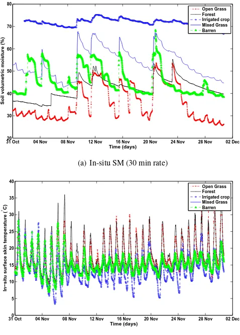
4.1 Near-surface SM variations based on LC type
Comparison of the in-situ measurements revealed significant dif-ferences in the volumetric soil moisture over various LC types. Greatest anisotropy from the dominant trend is seen on the irri-gated site, while the other LC types have relatively similar trends
over the field measurement period (Fig.2(a)). Spikes in the SM
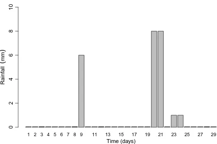
visible in most of the sites are due to rainfall events. This can be interpreted from the rainfall data. Although the rainfall data were only available in Birdlings Flat site (with LC type ‘Open grass’), the spikes in SM correspond to the rainfall events in most of the sites (e.g., 9th, 20thand 21stof November, see Fig.3). During the few hours after the rainfall events moisture levels drop signif-icantly. However, temperature trends dominantly follow day and
night maximum and minimums, respectively (Fig.2(b)). Apart
from the visual comparison, statistical analysis of the correlations between the two parameters was necessary to ensure if any long-term relationship exists between LST and SM in the area, which is discussed in the next section.
31 Oct20 04 Nov 08 Nov 12 Nov 16 Nov 20 Nov 24 Nov 28 Nov 02 Dec
(a) In-situ SM (30 min rate)
31 Oct0 04 Nov 08 Nov 12 Nov 16 Nov 20 Nov 24 Nov 28 Nov 02 Dec
In−situ surface skin temperature (
°C)
(b) In-situ surface skin temperature (30 min rate)
Figure 2: a. Variations of the near-surface (<5 cm depth) volu-metric soil moisture, and b. variations of surface skin temperature over different LC types during the field measurements (Nov-Dec. 2011)
4.2 Correlations between LST and SM time-series
1 2 3 4 5 6 7 8 9 11 13 15 17 19 21 23 25 27 29
Figure 3: daily rainfall in Birdlings Flat site during Nov. 2011
time-series of SM for the same period. To reveal the suspected linearity in the relationsship between the two parameter, non-linear regression analysis also used in the calculation, which did not provide any improvement in the results. This indicated that the relationship between LST and SM is more complicated and needs more careful data analysis. The same complication is
vis-ible when the single time-series of SM are considered (Fig.2).
Therefore, time-series of SM were divided into two series namely day and night series to capture the unique variations of SM in warmer and often drier daylight hours compared to cooler con-ditions of the night. Nevertheless, no significant improvement achieved from the correlation of day or night series save few cases (e.g., Barren LC type both day and night). As a consequence, time-series were broken into smaller periods.
4.3 Correlations between subsets of LST and SM time-series following rainfall events
Considering time-series of SM, break-points were chosen based on the higher points visible in the trends to overcome the sud-den effects of rainfall events. These higher points, as discussed earlier, correspond to rainfall events (see figures2(a)and2(b)), therefore, the expected normal SM and surface temperature trend is significantly interfered by these events. The challenge in this method was the limited available observations from MODIS LST, which is limited to four observations in clear and cloudless days. No significant improvement was observed in the correlations be-tween combined daily time-series, however, separate time-series of day and night showed considerable improvements (see
Ta-ble2). In this case the inverse correlations can be interpreted
from the negative Pearson’srvalues. Except for the daily
time-series of ‘Irrigated Crop’, all the cases have shown an inverse cor-relation between MODIS LST and the in-situ SM data. The dif-ference between day and night series correlation with that of the combined daily time-series is significant. As a result, it seems the relationship between LST and near surface SM varies from day to night, and a change in the direction of the correlation cannot be ruled out. This lead to an assumption of a nonlinear correlation between the two parameters. Hence, a non-linear (or curvilinear) correlation (NLC) fit with a quadratic model was used to calcu-late correlations between the two parameters. However, except for few cases, there was no considerable change in the
correla-tion results (see Table2, second column). Even though
corre-lations for the separate day and night series have increased, the results still are not substantial. This means the variations in the two variable happen even in smaller time-frames. Considering time-series of LST (Fig.2(b)), largest variations in surface tem-perature happen about every 12 hours. This can be a clue to look for a higher inverse correlation between LST and SM from the
LC Type r-daily NLCr-daily r-day r-night
Table 2: Pearson’srvalues from correlation of LST vs. in-situ
SM after rainfall event on 21stNov. to 1stDec. 2011 over
vari-ous LC types
Table 3: Pearson’sr values from correlation of in-situ surface
temperature vs. in-situ SM based on data from 21stof Nov. 2011
over various LC types
series of a single day. Therefore, breaking down the time-series to even smaller intervals could be one option to further increase the correlations, however, as mentioned before, there are not enough observations from the MODIS LST for a single day (or even a few days). As a consequence, correlations calculated using the in-situ measured surface temperature and SM data for a single day is discussed in the next section.
4.4 Correlations between in-situ surface temperature and SM for a single day
In this section correlations between surface temperature and near-surface SM in-situ data, both with 30 minute rate, from a sin-gle day are presented. As the previous sections, correlations are based on the combined daily time-series as well as the separated day and night series. Combined daily time-series from all the LC types showed significant improvement in the correlations (see Ta-ble3, first column). Day series correlations are ambiguous, some of the LC types showed positive while the other LC types showed relatively strong inverse correlations. Finally, the night series showed strong inverse correlations for all the LC types. Some of the LC types, such as forest and the irrigated site, showed lower correlations which seems is due to the unusual distribution of heat or moisture on the soil under the effects of the canopy.
5 CONCLUSIONS AND FUTURE WORK
reported by other works in the literature (Wilson et al., 2003). This implies that the study of SM based on remotely sensed LST using a statistical method can be possible if there is higher num-ber of observations available for a single day. Currently such a dataset is only available from the geostationary satellites such as the Spinning Enhanced Visible and Infrared Imager (SEVIRI) on-board the Meteosat Second Generation (MSG) satellite. How-ever, limitations with geostationary sensors include poor spatial resolution and high view angles for parts of the globe such as New Zealand. Nevertheless, considering the results from this pa-per, the authors look forward to the possibility of using a geosta-tionary satellite data for a further analysis similar to the objective of this paper.
ACKNOWLEDGEMENTS
This research is conducted under funding and support of the Uni-versity of Canterbury in New Zealand. The authors would like to thank Justin Harrison for his help in the field experiment which was conducted for this research. We also acknowledge Graeme Plank from the Physics Department for providing us the climate data, as well as permission for setting up our instrument in the Birdlings Flat site. Access to the NASA’s MODIS LST data is
also appreciated; we usedReverbtool to download this data.
REFERENCES
Bastiaanssen, W. G. M., 2000. SEBAL-based sensible and la-tent heat fluxes in the irrigated Gediz Basin, Turkey. Journal of Hydrology 229(1-2), pp. 87–100.
Bhagat, V. S., 2009. Use of Landsat ETM+ data for detection of potential areas for afforestation. International Journal of Remote Sensing 30(10), pp. 2607–2617.
Carlson, T. N., Gillies, R. R. and Perry, E. M., 1994. A method to make use of thermal infrared temperature and NDVI measure-ments to infer surface soil water content and fractional vegetation cover. Remote Sensing Reviews 9(1-2), pp. 161–173.
Grabs, T., Seibert, J., Bishop, K. and Laudon, H., 2009. Model-ing spatial patterns of saturated areas: A comparison of the topo-graphic wetness index and a dynamic distributed model. Journal of Hydrology 373(12), pp. 15 – 23.
Gruhier, C., de Rosnay, P., Hasenauer, S., Holmes, T., de Jeu, R., Kerr, Y., Mougin, E., Njoku, E., Timouk, F., Wagner, W. and Zribi, M., 2010. Soil moisture active and passive microwave products: intercomparison and evaluation over a Sahelian site. Hydrology and Earth System Sciences 14(1), pp. 141–156.
Hain, C. R., Crow, W. T., Mecikalski, J. R., Anderson, M. C. and Holmes, T., 2011. An intercomparison of available soil moisture estimates from thermal infrared and passive microwave remote sensing and land surface modeling. J. Geophys. Res. 116(D15), pp. D15107–.
Hassan, Q. K., Bourque, C. P.-A., Meng, F.-R. and Cox, R. M., 2007. A Wetness Index Using Terrain-Corrected Surface Temper-ature and Normalized Difference Vegetation Index Derived from Standard MODIS Products: An Evaluation of Its Use in a Hu-mid Forest-Dominated Region of Eastern Canada. Sensors 7(10), pp. 2028–2048.
Jackson, T. J., Schmugge, J. and Engman, E. T., 1996. Remote sensing applications to hydrology: soil moisture. Hydrological Sciences Journal 41(4), pp. 517–530.
LPDAAC, 2010. MODIS Reprojection Tool Swath User Manual. 47914 252nd Street Sioux Falls, SD 57198-0001 USA.
Rigo, G. and Parlow, E., 2005. Measurement and modeling of the ground heat flux in the city of Basel during BUBBLE by different methods. In: ISPRS Intl. Archives of Photogrammetry, Remote Sensing and Spatial Information Sciences, Vol. XXXVI PART 8/W27.
Rigo, G. and Parlow, E., 2007. Modelling the ground heat flux of an urban area using remote sensing data. Theoretical and Applied Climatology 90, pp. 185–199. 10.1007/s00704-006-0279-8.
Sørensen, R., Zinko, U. and Seibert, J., 2005. On the calculation of the topographic wetness index: evaluation of different meth-ods based on field observations. Hydrology and Earth System Sciences Discussions 2(4), pp. 1807–1834.
Sun, D. and Pinker, R. T., 2004. Case study of soil moisture effect on land surface temperature retrieval. IEEE Geoscience and Remote Sensing Letters 1(2), pp. 127 – 130.
Wan, Z., 1999. MODIS Land-Surface Temperature Algorithm Theoretical Basis Document: LST ATBD. Institute for Com-putational Earth System Science University of California, Santa Barbara, CA 93106-3060.
Wan, Z., 2008. New refinements and validation of the MODIS Land-Surface Temperature/Emissivity products. Remote Sensing of Environment 112, pp. 59–74.
Wan, Z. and Dozier, J., 1996. A generalized split-window
algorithm for retrieving land-surface temperature from space. Geoscience and Remote Sensing, IEEE Transactions on 34(4), pp. 892 –905.
Wan, Z., Zhang, Y., Zhang, Q. and Li, Z., 2004. Quality assess-ment and validation of the MODIS global land surface tempera-ture. International Journal of Remote Sensing 25, pp. 261–274.
Wang, C., Qi, J., Moran, S. and Marsett, R., 2004. Soil moisture estimation in a semiarid rangeland using ERS-2 and TM imagery. Remote Sensing of Environment 90(2), pp. 178 – 189.
Wang, L. and Qu, J., 2009. Satellite remote sensing applications for surface soil moisture monitoring: A review. Frontiers of Earth Science in China 3, pp. 237–247.
Wilson, D. J., Western, A. W., Grayson, R. B., Berg, A. A., Lear, M. S., Rodell, M., Famiglietti, J. S., Woods, R. A. and McMahon, T. A., 2003. Spatial distribution of soil moisture over 6 and 30 cm depth, Mahurangi river catchment, New Zealand. Journal of Hydrology 276(14), pp. 254 – 274.