THE EARLY DETETCTION OF THE EMERALD ASH BORER (EAB) USING
ADVANCED GEOSPATIAL TECHNOLOGIES
B. Hu a, *, J. Li a, J. Wang a, and B. Hall b
a
Dept. of Earth and Space Science and Engineering, York University, 4700 Keele St, Toronto ON M3J1P3 Canada – [email protected], [email protected], [email protected]
b
Esri Canada, 12 Concorde Place Suite 900, Toronto ON M3C 3R8,Canada – [email protected]
Technical Commission II
KEY WORDS: Hyperspectral, LiDAR, Very high spatial resolution imagery, Species identification, Emerald Ash Borer, Tree health
ABSTRACT:
The objectives of this study were to exploit Light Detection And Ranging (LiDAR) and very high spatial resolution (VHR) data and their synergy with hyperspectral imagery in the early detection of the EAB presence in trees within urban areas and to develop a framework to combine information extracted from multiple data sources. To achieve these, an object-oriented framework was developed to combine information derived from available data sets to characterize ash trees. Within this framework, individual trees were first extracted and then classified into different species based on their spectral information derived from hyperspectral imagery, spatial information from VHR imagery, and for each ash tree its health state and EAB infestation stage were determined based on hyperspectral imagery. The developed framework and methods were demonstrated to be effective according to the results obtained on two study sites in the city of Toronto, Ontario Canada. The individual tree delineation method provided satisfactory results with an overall accuracy of 78% and 19% commission and 23% omission errors when used on the combined very high-spatial resolution imagery and LiDAR data. In terms of the identification of ash trees, given sufficient representative training data, our classification model was able to predict tree species with above 75% overall accuracy, and mis-classification occurred mainly between ash and maple trees. The hypothesis that a strong correlation exists between general tree stress and EAB infestation was confirmed. Vegetation indices sensitive to leaf chlorophyll content derived from hyperspectral imagery can be used to predict the EAB infestation levels for each ash tree.
* Corresponding author.
1. INTRODUCTION
Emerald Ash Borer (EAB, Agrilus planipennis Fairmaire) is an invasive insect species that attacks all species of ash trees (Fraxinus spp) (Maloney et al., 2006, and Sydnor et al., 2007). It was first found in North America in 2002 and has become established in several states in the United States of America and in Ontario, Canada (Kovacs et al., 2010). The beetle has caused the death of millions of ash trees during the past decade (Rose, 2010). Despite substantial research and control efforts, the beetle has continued to spread to new areas. The ash trees attacked by EABs typically die within 3 to 5 years and often show serious decline within 2 years. Due to the aggressive nature of EAB infestation, the earliest possible detection of the infestation is crucial to help reduce the spread and damage of EAB. It would be ideal to be able to detect the beetle when its density is still low and before signs and symptoms are obvious (Ryall et al. 2011). Commonly used methods include sticky traps baited with an attractant and branch sampled gallery counts (Ryall et al., 2011). Even though these field survey methods have been proved effective, they are labour-intensive and time-consuming. Alternative solutions have sought to exploit the increasingly available hyperspectral remote sensing technologies.
Hyperspectral sensors record hundreds of narrow and contiguous measurements of electromagnetic energy reflected by an object typically in the spectral ranges of from 400 nm up to 2500 nm. Thus, subtle differences in the reflectance patterns
within the working range of a hyperspectral sensor may be detected. Studies have shown that hyperspectral remote sensing data, with their fine spectral resolution, can be used to detect early signs of stress and sometimes even when the stress symptoms are not visible to the human eye (e.g, Carter, 1993; Carter and Miller, 1994; Pontius et al., 2005). This is because stressed leaves tend to have reduced photosynthetic activity and chlorophyll content and thus have slightly different reflectance patterns in the visible and near-infrared spectrum, compared with health leaves of the same species. Hence, the stress-induced changes in the reflectance may be detected by hyperspectral sensors.
In the case of EAB infestation, EAB larvae feed between the sapwood and bark along the trunk of a tree, which cuts off the flow of water and nutrients and causes visible stress to the tree. In the past several years, studies have been conducted to assess the capabilities of commercially available hyperspectral sensors to predict ash tree decline caused by EAB infestation. In Pontius et al. (2008), hyperspectral SpecTIR imagery with a spatial resolution of 1m by 1m was used to map ash decline at the landscape level in forests in Michigan and Ohio. It was reported that 71% of the variability in ash decline was accounted for with 6 vegetation indices sensitive to leaf chlorophyll content and water content. Since plant-physiological responses to stress are similar regardless of the cause of stress (Chapin, 1991), Pontius et al. (2008) could not conclude that declining trees identified in their study areas were infested with EAB.
Souci et al. (2009) reported an EAB detection project in the city of Milwaukee, USA using hyperspectral SpecTIR imagery (with a spatial resolution of 1 m by 1m) and LiDAR (Light Detection And Ranging) data. In their project, ash trees were classified from hyperspectral imagery using training samples and the results were improved by information derived from LiDAR data using geographic information system (GIS) tools. The classification was deemed to be successful, even though quantitative assessment was not reported. They also concluded that it was critically important to collect numerous field spectra from diverse trees in terms of spatial location, species, state, and understory composition.
Hanou (2010) demonstrated successful use of hyperspectral SpecTIR imagery to map ash trees within the town boundary of Oakville, Ontario Canada with classification accuracy of 81% and promising results with the prediction of EAB infestation level by the vegetation index of (Rswir+RGreen)
2
/ (Rswir-RGreen), where Rswir and RGreen are the reflectance in one channel in the spectral range of short wave infrared and green, respectively. Based on a limited number of EAB observations obtained using branch sampling methods (Ryall et al. 2011), it was confirmed that EAB infestation, as defined by the number of galleries per trunk area at the breast height, was found to be highly correlated with above mentioned vegetation index calculated from ground-based reflectance spectra (measured by an ASD spectrometer). The correlation became weaker if the index was calculated from aerial hyperspectral imagery (with a spatial resolution of 1m by 1m). This was primarily due to the fact that the digital value associated with a pixel in the hyperspectral imagery may contain a mix of the energy reflected from the objects within the foot-print of this pixel. The mixture was especially higher for trees with less crown coverage or thin canopies. The reflectance for a pixel in this situation was likely a composition of species-specific and understory reflectance which influence species mapping and infestation detection Hanou (2010). Continuing with the efforts of Hanou (2010), Zhang et al (2014) improved the prediction of EAB infestation by combining spectral and spatial information derived from the hyperspectral SpecTIR imagery and high spatial resolution Google Earth imagery, respectively. The prediction accuracy was 0.625, compared with the branch sampling methods (Ryall et al. 2011). An object-oriented method was employed with individual tree crowns as the basic units. However, the individual ash trees were delineated manually based on the information provided by the town of Oakville.
Building on the research work of the above mentioned studies, in this paper we establish a framework to identify ash trees automatically and effectively and characterize their EAB infestation stages within urban environments using hyperspectral imagery, together with very high spatial resolution imagery and LiDAR data. The latter data sets provided not only complementary information contributing directly to ash tree identification and EAB infestation detection, but also information to improve the interpretation of hyperspectral imagery by alleviating any issues associated with its relative low spatial resolution. To integrate effectively information from different sources, we adopted an object-oriented approach and employed individual tree crowns as the basic unit. For the first time, a complete work flow from individual tree crown delineation to ash tree identification to the characterization of EAB infestation was proposed. Acknowledging that for a given study area, not all of these data sets are available, we designed the method at each step in order
to employ the maximized values of each data set whenever it was available. The developed methods were tested over two study sites in the city of Toronto, Ontario Canada.
2. STUDY AREAS AND DATA USED
Based on the availability of remote sensing data and site accessibility, two areas were selected for this study in the city of Toronto, Ontario Canada: the Keele campus of York University and a neighborhood near highway 404 and Shepard Avenue in the north east area of the city.
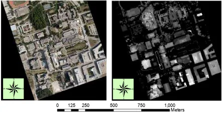
For the site on the Keele campus of York University (43.77165°N, 79.501321°W)) (hereafter referred as Site 1), both very high spatial resolution imagery and airborne LiDAR data acquired in the summer of 2007 were available. The imagery had a spatial resolution of 0.5 m and 0.5 and four broad bands covering the spectral regions of red, green, blue and near-infrared. The pulse density of the LiDAR data was 1 pulse per square meter. A digital elevation model (DEM) and digital surface model (DSM) with the same spatial resolution as the imagery were subsequently generated from the LiDAR data cloud. To generate the DSM, all the first-return LiDAR points within each grid cell were selected, a maximum height value of the points was used to fill the cell, and any empty cell was filled by interpolating the values of non-zero neighbour cells (Hyyppä et al., 2001; Pitkänen et al., 2004). To generate the DEM, ground surface points were iteratively selected from all of the LiDAR points and then interpolated to form the DEM (Hyyppä and Inkinen, 1999; Hyyppä et al., 2001). The CHM was derived as the difference between the DSM and DEM, which was then smoothed with a 3 by 3 Gaussian low-pass filter to eliminate noise, as used in Hyyppä et al. (2001) and Morsdorf et al. (2004). The colour composite VHR image and LiDAR CHM are shown in Figure 1. Using the data sets in this study site, we tested the methods for individual tree crown delineation and ash tree identification.
0 125 250 500 750 1,000
Meters
Figure 1. The true colour composite VHR imagery (left) and LiDAR CHM (right) covering the Keele campus of York University (Site 1) (43.77165°N, 79.501321°W).
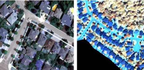
The data available for the neighborhood of highway 404 and Shepard Avenue (43.777503°N, 79.339701°W) (hereafter referred as Site 2) included the hyperspectral imagery acquired by a CASI (Compact Airborne Spectrographic Imager) instrument in 2009, and very high spatial resolution imagery (2009), as shown in Figure 2. The CASI imagery had a spatial resolution of 1 m by 1 m and 9 spectral bands with a bandwidth of 5nm covering from 400 to 900 nm. It was processed to at-ground reflectance data through calibration, atmospheric correction and geo-referencing. The very high spatial resolution imagery had a spatial resolution of 0.5 m and 0.5 and four broad bands covering the spectral regions of red, green, blue and
infrared. A limited number of trees were sampled for signs of EABs in 2008 and in 2013. The data sets in this area were used to test the developed methods in terms of individual tree delineation, ash tree identification and the characterization of EAB infestations.
Figure 2. The true colour composite VHR imagery (left) and false colour composite of the CASI imagery covering Site 2 (43.777503°N, 79.339701°W).
3. METHODS
The basic idea underlying the developed methods was as follows: individual trees were first extracted from VHR imagery and LiDAR data if available and treated as basic units for subsequent analyses. These trees were then classified into different species based on available information, such as their spectral information derived from hyperspectral imagery and spatial information from VHR imagery. For each ash tree, its state of health and EAB infestation stage were determined.
3.1 Individual tree crown (ITC) delineation
In recent decades, various methods have been developed to detect or delineate ITCs from VHR imagery, LiDAR data, or their combination (Jakubowki et al., 2013). In this study, the multi-scale method developed by Jing et al (2013) and Hu et al (2014) was adopted to account for the trees of various sizes in the study areas. It was based on marker-controlled watershed segmentation (Beucher and Lantuejoul, 1979, and Meyer and Beucher, 1990). However instead of using tree tops as markers, as most of the ITC delineation methods, the method used in this research employs horizontal cross-sections to minimize noise effects in the data and false positives and negatives caused by the complex structures of canopies in deciduous and mixed-wood forests. Two modifications were made to the original ITC method (Jing et al., 2013 and Hu et al., 2014). A mask of pixels representing non-trees was generated first and these pixels were set to zero in the subsequent delineation process. After tree tops were identified, a region growing method was used to delineate each tree crown instead of the watershed segmentation approach used by Jing et al (2013) and Hu et al. (2014). With these two improvements, prior knowledge on the trees of interest can be readily incorporated. In the following, the ITC delineation method used is described in detail on a step-by-step basis.
3.1.1 The generation of a mask of non-tree pixels: A
rule-based approach was used to generate a mask of non-tree pixels based on three features. The normalized difference vegetation index (NDVI) calculated using the brightness values in the red and near-infrared bands of the VHR imagery was used to separate tree and non-tree pixels. To separate pixels of grass and trees, the CHM was used if LiDAR data available. Otherwise, the local variance calculated from the brightness values within an 11 by 11 window in the near-infrared band of the VHR imagery was used. The rules used to generate the mask stated as follows. A pixel was identified as non-tree if the values of its NDVI and CHM were smaller than 0.15 and 2 m, respectively, if LiDAR data were available. Otherwise, a pixel was identified as non-tree if the values of its NDVI and local variance were smaller than 0.15 and thr, respectively. thr was determined automatically based on the mean and standard deviation of the local variances within vegetation pixels. The thresholds for NDVI and CHM were determined empirically.
3.1.2 The identification of tree tops: Individual tree tops
were determined from the CHM image, if available, or the first principal component generated by principal component analysis (PCA) of the VHR imagery using the method described in Hu et al (2014).
3.1.3 Seeded region growing: With the identified tree tops,
region growing with the local mutual best fitting was first performed based on the Euclidean distance between the spectral reflectance in the four bands of two neighboring segments. This process was repeated until none of adjacent segments could be merged. As expected, after this region growing procedure, a number of segments with a small number of pixels existed and some segments did not have “round” crown shapes. As a result, small segments were then merged and the merging process was controlled by the shape factor (SF) defined in equation (1).
RA A
SF (1)
In Equation (1), A was calculated as the total number of pixels covered by any two segments to be merged and RA as the number of pixels covered by the rectangle bounding the resulting areas after merging these two segments. Two adjacent segments were merged if their reflectance was similar (smaller than a threshold) and their shape factor was smaller than 0.4. The threshold value of 0.4 was determined, because it is the best value to distinguish between strips and circles. In order to generate a crown segment map with relatively realistic tree crown shapes, the following post processing was designed to smooth the crown boundary.
For a data set with LiDAR data, the seeded pixels were sorted based on their heights using the LiDAR CHM. The segment with highest seed pixel had the priority to be smoothed than that with a seed pixel of lower height value. The reason is that when two trees grow close to each other, the taller tree tends to have a more integrated crown shape than the lower one. To smooth any chosen segment, the boundary pixels in the segment were identified. With the seed point in the segment as the reference point, the azimuth angle of each boundary pixel and its distance (referred to as the radius) were calculated. If multiple boundary pixels occurred in one azimuth direction, the radius at that azimuth angle was computed as the mean value of all calculated radii. For each seed pixel, its corresponding edge pixels were sorted based on the azimuth angle from zero to 360 degrees. Then a 5x1 mean filter was applied to the radius of each crown
segment. For the case of no radius was found at one azimuth angle, the radius was linearly predicted through two adjacent directions.
3.2 Identification of individual ash trees
For the individual tree crowns obtained using the method described in Section 3.1, a total of 10 spectral and 2 texture features were derived from the VHR image. The spectral features included mean and variance of the brightness values in the four spectral bands, mean greenness index (GI) and mean green-red index (GRI):
blue green red
green
R R R
R GI
(2)
red green
red green
R R
R R GRI
(3)
where
blue green
redR R
R , , = brightness values in the spectral bands
of red, green and blue of the VHR imagery
The texture features were the statistics of homogeneity and contrast were calculated from the grey-level co-occurrence matrix (GLCM) (Haralick, 1973). These 12 total features were used to classify individual trees into four categories: ash, maple, other deciduous trees, and conifers. A generalized linear model was created for this purpose using stepwise regression. Stepwise regression is a systematic method for adding and removing terms from a linear or generalized linear model based on their statistical significance in explaining the dependent variable (Dobson 1990). The dependent variable comprised integers from 1 to 4, representing the four classes, respectively. The independent variables were the 12 features. Once a generalized linear regression model was created using training samples of individual trees, the prediction of the dependent variable for all trees in the entire study area was performed based on the obtained model. The value of the predicted dependent variable (i.e., species class) for each tree was then stored to create a prediction map. Based on the model set-up, the closer to 1 the predicted value was, the more likely the tree was ash. The created map is an indication of the likelihood of the species class that a tree belongs to. To identify ash trees clearly, a range of the likelihood was selected by a lower and upper threshold. In this way, a binary class map indicating ash and non-ash trees was finally created.
3.3 Characterization of EAB infestation
As mentioned earlier, unhealthy vegetation typically exhibits different compositions of pigment content and water content (among other things), which can be characterized by a number of vegetation indices derived from multispectral and hyperspectral remote sensing imagery. By examining existing vegetation indices, the five indices listed in Table 1 were used to distinguish healthy and unhealthy ash trees. The stepwise regression of a generalized linear model was then performed with the five indices as independent variables and the dependable variable taking values of 0 (healthy ash tree) and 1 (unhealthy ash trees).
Vegetation
Indices Equation Physical relation
GI (Smith et al., 2005)
R554/R677 Leaf area index; chlorophyll content GMb (Gitclson
and Mcrzlyak, 1994)
R750/R700 Total chlorophyll content
The ratio of TCARI and OSAVI (Haboudane, et al., 2004)
TCARI=3(R700-R670 )-0.2(R700
-R550)(R700/R670) OSAVI=1.16(R800 -R670)/(R800+R670+0.16)
Total chlorophyll content
PRI (Mcrzlyak et al., 1999)
(R531-R570)/(R537+R570) Carotenoid
NDVI (R864-R710)/(R864+R710) Vegetation cover Table 1: The selected vegetation indices, where R represents the surface reflectance at the specific wavelength. For example, R554 means the surface reflectance value of the pixel at the 554 nm.
4. RESULTS AND DISCUSSION
4.1 ITC delineation
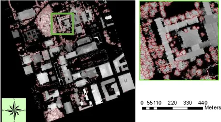
The ITC delineation method was applied to VHR imagery and LiDAR data over Site 1 and VHR imagery over Site 2 (Figure 1). The individual tree crowns delineated are shown in Figure 3 and Figure 4, respectively. It is clear that most of the trees were delineated correctly. To assess the delineation accuracy, we manually delineated the crowns in Site 1 based on our visual interpretation of the digital image and used these as reference points. Based on the criteria described in Hu et al (2014), the overall accuracy of an automatically generated map of individual tree crowns was 78%, with 19% commission and 23% omission errors.
055110 220 330 440 Meters
Figure 3. Individual tree crowns delineated from the VHR imagery and LiDAR CHM data overlaid with LiDAR CHM in Site 1.
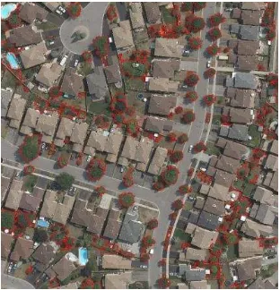
Figure 4. Individual tree crowns delineated from the VHR imagery in Site 2.
4.2 Identification of individual ash tree
For Site 1, the predicted result and identified ash trees are shown in Figure 5 and Figure 6 (white segments), respectively. The predicted values in Figure 5 were useful because they provided information on the likelihood that a given tree belonged to a specific class, and by adjusting the thresholds of regression value dynamically, users can possibly obtain more accurate classification results based on their own knowledge of different study areas. The classification results were validated using 104 sampled trees whose species were determined in the field. Among these, there were 24 ash, 35 maple, 23 other deciduous, and 22 coniferous trees. For each class, about 70% of the trees were randomly selected as training samples and the remaining trees were used for testing. As a result, out of the 24 ash tree samples, 16 were used for training and 8 for testing. The results correctly identified 6 of the ash testing samples (75%). In addition, 4 non-ash trees were incorrectly identified as ash (commission error 15%), and 2 ash trees were incorrectly identified as non-ash trees (omission error 25%).
M
Regression value of Species Classes of Trees in York University
Figure 5. The regression value of the classes of tree species, together with the locations of the sampled ash trees.
79°30'0"W
Identified Ash Trees in York University
Legend
Figure 6. The identified ash trees in Site 1 by thresholding the regression values.
The classification results for Site 2 are shown in Figure 7. The species of the trees in this area were also determined in the field. All of the ash trees (11) in this area were correctly classified. However, 3 non-ash trees were incorrectly classified as ash trees.
Regression Map of East Toronto Site
0 1020 40 60 80
Meters
Ash and Non-Ash of the East Toronto Site
Legend
Figure 7. The identified ash trees in Site 2 by thresholding the regression values.
4.3 Characterization of EAB infestation
Based on the results conducted using a branch sampling approach in 2009 and field inspection in 2013, a limited number of ash trees in Site 2 were selected as training samples for the generalized regression analysis (Section 3.3) using the vegetation indices in Table 1. The regression values predicted (Figure 8) suggested healthy and unhealthy could be well separated if a single threshold (e.g., 0.5) was applied.
Figure 8. Regression values for the prediction of healthy and unhealthy ash trees in Site 2.
Due to the limited number of ash trees and also EAB-infested ash trees in Site 2, we validated our method using the data in the town of Oakville used by Zhang et al (2014) and Hanou (2010). In total, 33 ash tree samples were selected, including 26 healthy and 7 EAB-infested unhealthy ash trees. Our predictive model resulted in an overall success rate of about 70%.
5. CONCLUSIONS
The framework developed to identify ash trees and characterize their EAB infestation was demonstrated to be promising based on our limited test samples in the two study sites in the city of Toronto, Ontario, Canada. However, further validation is needed.
With the framework, object-oriented methods were developed to integrate effectively information from different remote sensing data. The fusion of spectral and height information derived from VHR imagery and LiDAR data proved to be necessary and effective in the delineation of individual tree crowns. With our ITC delineation method, satisfactory results were obtained.
In terms of the identification of ash trees, 12 spectral and textual features calculated for each tree crown were used. The selection of important features was performed using stepwise regression combined with the generalized linear model. Detailed analysis of the significance of these features is currently under investigation. Based on the classification result, one tree could be classified as ash or non-ash with a probability of how much it belonged to ash. Tests conducted at two different study sites demonstrated satisfactory results. In this study, we did not include LiDAR data in the step of ash tree identification because the low density of the available LiDAR data could not contribute sufficient information for species identification. However, LiDAR data can be easily added into our classification model if high density LiDAR data are available. Caution should be taken in that the classification tests were based on a few training and testing samples, and further research with more field samples is needed.
The use of hyperspectral data to quantify the health of ash trees achieved expected results. Unhealthy ash trees exhibited lower reflectance at the red edge and NIR bands than healthy ash trees. The five vegetation indices used in this study proved to be very useful in the separation between healthy and unhealthy ash
trees. Although we did not have significant unhealthy ash tree samples for use in this study, the 70% success rate in our binary classification (healthy/unhealthy) result indicates the feasibility of using hyperspectral data to predict presence/absence of EAB ash tree infestation. If more samples were available for training, it is likely that better results would have been obtained.
ACKNOWLEDGEMENTS
The authors would like to thank Ziya He and Meaghan Eastwood of Toronto and Region Conservation for their contributions in the field and in consulting this research, the town of Oakville, AMEC Inc. and York University library for the kindly supplying the data and technical support, and Dr. Krista Ryall of Canadian Forest Service for the ground truth data in the Toronto stud site. The authors are also grateful for financial support provided by the Natural Sciences and Engineering Research Council (NSERC) of Canada.
REFERENCES
Beucher, S., and Lantuejoul, C. 1979. Use of watersheds in contour detection, International Workshop on Image Processing, Realtime Edge and Motion Detection/Estimation, 17-21 September 1979, Rennes, France, pp. 12-21.
Carter, G. A. 1993. Responses of leaf spectral reflectance to plant stress. American Journal of Botany,80, 239−243.
Carter, G. A., and Miller, R. L., 1994. Early detection of plant stress by digital imaging within narrow stress-sensitive wavebands, Remote Sensing of Environment, 50, 295-302.
Chapin, F. S., 1991. Integrated responses of plants to stress.
Bioscience, 41, 29−36.
Gitelson, A. A., & Merzlyak, M. N. 1994. Quantitative estimation of chlorophyll-a using reflectance spectra: Experiments with autumn chestnut and maple leaves. Journal of Photochemical Phytobiology, 22, 247−252.
Haboudane, D., Miller, J.R., Pattey, E., Zarco-Tejada, P.J., and Strachan, I.B., 2004. Hyperspectral vegetation indices and novel algorithms for predicting green LAI of crop canopies: Modeling and validation in the context of precision agriculture,
Remote Sensing of Environment, 90, 337-352.
Hanou, I., 2010. Town of Oakville Hyperspectral EAB Analysis, Town of Oakville government document.
Haralick, R.M., Shanmuga, K. and Dinstein, I., 1973. Textural Features for Image Classification. IEEE Transactions on Systems Man and Cybernetics, Smc3(6): 610-621.
Hu, B., Li, J., Jing, L. and Judah, A., 2014. Improving the efficiency and accuracy of individual tree crown delineation from high-density LiDAR data, International Journal of Applied Earth Observation and Geoinformation, 26, 144-155.
Hyyppä, J. and Inkinen, M. 1999. Detecting and estimating attributes for single trees using laser scanner, The
Photogrammetric Journal of Finland, 16(2):27–42.
Hyyppä, J., O. Kelle, M. Lehikoinen, and M. Inkinen, 2001. A segmentation-based method to retrieve stem volume estimates
from 3-D tree height models produced by laser scanners, IEEE Transactions on Geoscience and Remote Sensing, 39(5):969– 975.
Jakubowski, M. K., Li, W., Guo, Q. and Kelly, M. 2013. Delineating individual trees from Lidar data: A comparison ofvector- and raster-based segmentation approaches. Remote Sensing, 5, 4163-4186.
Jing, L., Hu, B., Li, L., Noland, T., and Guo, H., 2013. Automated tree crown delineation from imagery based on morphological techniques”, 35th International Symposium o Remote Sensing of Environment, Beijing, 22-26 April 2013
Kovacs, K. F., Haight, R. G., McCullough, D. G., Mercader, R. J., Siegert, N. W., and Liebhold, A. M., 2010. Cost of potential emerald ash borer damage in U.S. communities, 2009 – 2019,
Ecological Economics, 69(3), 569-578.
Maloney, K., Boughton, J., Schneeberger, N., 2006. Emerald Ash Borer 2006 Brief, Newtown Square, PA, USDA Forest Service, Northeastern Area, State and Private Forestry, USA.
Meyer, F., and Beucher, S., 1990. Morphological segmentation, Journal of Visual Communication and Image Representation, 1(1):21–46.
Merzlyak, M. N., Gitelson, A. A., Chivkunova, O. B., and Rakitin, V. Y., 1999. Non-destructive optical detection of pigment changes during leaf senescence and fruit ripening,
Physiologia Plantarum, 106, 135-141.
Morsdorf, F., Meier, E., Kötz, B., Itten, K. I., Dobbertin, M., and Allgöwer, B., 2004. LIDAR-based geometric reconstruction of boreal type forest stands at single tree level for forest and wildland fire management, Remote Sensing of Environment, 92(3):353–362.
Pitkänen, J., Maltamo, M., Hyyppä, J. and Yu, X. 2004. Adaptive methods for individual tree detection on airborne laser based canopy height model, Proceedings of ISPRS Working Group VIII/2: Laser-Scanners for Forest and Landscape Assessment, 3-6 October 2004, Freiburg, Germany, pp. 187– 191.
Pontius, J., Martin, M., Plourde, L., and Hallett, R., 2008. Ash decline assessment in emerald ash borer-infested regions: A test of tree-level, hyperspectral technologies, Remote Sensing of Environment, 112, 2665 – 2676.
Rose, J. R. 2010. Landowners Guide for Woodlot threaded by Emerald Ash Borer, Ontario Ministry of Natural Resource.
Ryall, K. L., Fidgen, J. G., and Turgeon, J. J., 2011. detectability of the emerald urban tree by using branch Samples,
Environmental Entomology, 3:40, 679 – 688.
Smith, A.M., Nadeaum, C., Freemantle, J. I. H., Teillet, P.M., Kehler, I.,Daub, N., Bourgeois, G., and de Jong, R.,2005. Leaf area index from CHRIS satellite and application in plant yield estimation, Proceeding of 26th Canadian Symposium on Remote Sensing, Wolfville, Nova Scotia.
Sydnor, T. D., Bumgardner, M., and Todd, A., 2007. The potential economic impacts of emerald ash borer on Ohio US Communities, International Society of Arboriculture, 1:33, 45-54.
Pontius, J. A., Hallett, R. A., & Martin, M. E., 2005. Assessing hemlock decline using hyperspectral imagery: Signature analysis, indices comparison and algorithm development.
Journal of Applied Spectroscopy, 59, 836−843.
Souci, J. S., Hanou, I, and Puchalski, D., 2009. High resolution remote sensing analysis for early detection and response planning for emerald ash borer, Photogrammetric Engineering and Remote Sensing, 905-909.
Zhang, K., Hu, B., and Robinson, J. 2014. Early detection of Emerald Ash Borer (EAB) infestation using multi-sourced data: a case study in the town of Oakville, Ontario, Canada.
International Journal of Applied Remote Sensing, Accepted for publication.