LOCALLY REFINED SPLINES REPRESENTATION FOR GEOSPATIAL BIG DATA
T. Dokkena, V.Skyttb and O. Barrowcloughc
SINTEF ICT, Department of Applied Mathematics, PO. Box 124 Blindern, 0314 Oslo, Norway a
[email protected], [email protected], [email protected]
Commission II, WG II/2, and WG II/6; Commission III, WG III/5; Commission IV, WG IV/3
KEY WORDS: Big data, smooth shape, splines, local refinement, elevation model
ABSTRACT:
When viewed from distance, large parts of the topography of landmasses and the bathymetry of the sea and ocean floor can be regarded as a smooth background with local features. Consequently a digital elevation model combining a compact smooth representation of the background with locally added features has the potential of providing a compact and accurate representation for topography and bathymetry. The recent introduction of Locally Refined B-Splines (LR B-splines) allows the granularity of spline representations to be locally adapted to the complexity of the smooth shape approximated. This allows few degrees of freedom to be used in areas with little variation, while adding extra degrees of freedom in areas in need of more modelling flexibility. In the EU fp7 Integrating Project IQmulus we exploit LR B-splines for approximating large point clouds representing bathymetry of the smooth sea and ocean floor. A drastic reduction is demonstrated in the bulk of the data representation compared to the size of input point clouds. The representation is very well suited for exploiting the power of GPUs for visualization as the spline format is transferred to the GPU and the triangulation needed for the visualization is generated on the GPU according to the viewing parameters. The LR B-splines are interoperable with other elevation model representations such as LIDAR data, raster representations and triangulated irregular networks as these can be used as input to the LR B-spline approximation algorithms. Output to these formats can be generated from the LR B-spline applications according to the resolution criteria required. The spline models are well suited for change detection as new sensor data can efficiently be compared to the compact LR B-spline representation.
1. INTRODUCTION
1.1 Smoothness of topography and bathymetry
Digital elevation models (DEM) can be considered to consist of either digital terrain models (DTM), which represent only the underlying topographic or bathymetric terrain, or digital surface models (DSM), which also include objects on the surface, such as buildings, vegetation etc. Typically DTMs are dominated by smooth regions of terrain with details and features occurring locally. Consequently, smooth representations are potentially well suited to modelling DTM data in a compact and accurate way. In order to include all the features that make up a DSM, these smooth representations should be complemented with alternative representations that are able to model sharp and discontinuous features. In IQmulus we have focused on the use of LR B-splines as the approach for representing the smooth background shape. In this paper, we propose a hybrid model for representing DEM data, which also includes triangulated irregular networks and point clouds.
2. REPRESENTATION OF DIGITAL ELEVATION MODELS
We will in this paper concentrate on locally refined spline representations; however, as such representations are not traditionally used for the representation of geospatial data we will first provide a short discussion of different approaches for the representation of digital evaluation models, and relate the locally refined spline representations to these.
2.1 Triangulated irregular network
The data used for building digital elevation models most often come from remote sensing in the form of sets of big point clouds. A triangulated irregular network (TIN) can be created directly from the point clouds. To reduce the data bulk the triangulation can be locally adapted to the complexity of the shape to reduce the data size and represent the shape within guaranteed tolerances. A TIN is composed of a data structure of irregularly distributed vertices (x,y,z) connected by edges that are boundaries of triangles. Algorithms using TIN-representation require traversing of the data structure of the triangulation, a process that is resource consuming.
2.2 Raster representation
A commonly used approach is to represent the digital elevation as a regular structure with vertices defined by a raster of points. The regularity of the raster grid contributes to speeding up algorithms. A raster, however, does not have local adaptation, thus important details might be lost if the resolution of the data is too low. On the other hand, high resolutions result in large amounts of data, much of which is often redundant. The shape inside a gridded element can be defined by a bilinear interpolation of the elements four corner points, or by splitting the element into two or more triangles.
2.3 Tensor product B-splines
bi-quadratic or bi-cubic B-splines. If the raster represents a very smooth shape interpolation may give very good shape descriptions. However, bi-quadratic or bi-cubic interpolation will be disturbed by distortions from a smooth behaviour. Consequently B-spline approximation methods that don't reproduce all small distortions will be more feasible. Similar to raster representation tensor product B-splines using uniform knots does not allow local adaptations of the granularity of the representation to the complexity of the shape of addressed. Tensor product B-splines with non-uniform knot vectors does not solve this problem as the topological structure of the polynomial elements remains a regular grid.
2.4 Locally refined splines
There are three main approaches to the local refinement of splines:
1. Hierarchical B-splines (Forsey et al., 1988) introduced a
wavelet like approach for shape representation using a hierarchical structure of B-splines at different refinement levels. Conditions that ensure linear independence of the resulting B-splines were introduced by (Kraft, 1996). Truncated Hierarchical B-Splines (Giannelli et al., 2012) provide an alternative formulation for Hierarchical B-splines with improved numerical properties.
2. T-splines (Sederberg et al., 2003) provide designers novel
functionality in creative freeform design. The approach is an algorithmic approach to local refinement of the B-spline vertex mesh, replacing the regular B-spline vertex mesh with a vertex mesh allowing T-junctions. However, until the introduction of Isogeometric Analysis (IGA) in 2005 (Hughes et al., 2005) locally refined splines got little attention. In IGA B-splines replace the shape functions of traditional finite elements, and thus allow higher order elements and allow higher order continuity between elements so reducing the data bulk of the representation. 3. Locally Refined B-splines (LR B-splines), (Dokken et al.,
2013) builds a theory for locally refined splines compatible with the traditional univariate Non-Uniform B-splines. The approach of LR B-splines provides a richer set of refinements than Hierarchical B-splines and T-splines, and includes with some few exceptions the spline spaces generated by the other approaches.
The main advantage of local spline refinement is that detail can be added locally, without increasing the amount of data globally. This contrasts with both raster and tensor-product spline formats in which data amounts increase globally with increased resolution. Locally refined splines also provide compact representations of smooth shapes, and are thus well suited to smooth terrains. The first results of the use of LR B-splines for the representation of geospatial data are presented in (Skytt et al., 2015).
2.5 Hybrid representations
Smooth and none smooth regions in a geospatial data set cannot efficiently be described using a single representation method. In addition geospatial point clouds occasionally contain outliers that are not part of the geospatial shape. A hybrid representation consisting of the following components can consequently be very attractive:
• LR B-spline representation for the smooth components (e.g., underlying terrain);
• triangulations for none smooth components (e.g., buildings and sharp features);
• point sets representing that cannot be represented by LR B-splines or triangulations, within the tolerance required.
This approach has the potential to efficiently represent the information embedded in geospatial point clouds. As the representation keeps all points outside the tolerance there is no need at this stage in to decide which are real points and what are outliers.
In the examples we show in this paper we do not use triangulations, rather we use LR B-spline surface approximations for modelling the underlying terrain from point cloud input. The points are then classified according to their distance from the surface and those that remain out-of-tolerance can be passed to algorithms for further processing. This is a first step in the implementation of our planned hybrid representation.
We have observed that frequently the points that remain outside the approximation tolerance are clustered locally. These clusters can represent different geometric configurations:
• Smooth shapes that are not detected by the current implementation of the LR B-spline approximation. Here we foresee that future improvements in the approximation algorithms will reduce the number of points in this category.
• None smooth shapes that are well suited for representation by triangulations.
• Collections of points that are not well suited for spline and triangle approximation. Some of these points will be outliers. Other might represent small features with too few points to be represented by a triangulation.
Combining a smooth locally refined spline representation with detailed modelled by TIN has the potential to provide a compact and accurate shape representation for digital elevation models. Access to cadastral data can help separate natural shapes from human made structures and shapes thus giving guidance concerning what should be represented by LR B-splines and what should be represented by TIN.
2.6 Compression of digital elevation representations
2.7 2.5D and 3D data representation
Typically elevation models are represented as 2.5D, meaning that for each horizontal point in the 2D plane, there is a single corresponding height value. It is also possible to model the full 3D representation. Triangulations provide the easiest way to model overhanging features such as cliffs and caves, and features of non-trivial topology such as bridges and tunnels. For visualisation purposes, triangular meshes can be smoothed using subdivision techniques (Pfeifer, 2005). Spline representations can also provide fully parametrized surfaces that can model overhanging features, but features of complex topology are more difficult. In the context of hybrid representations one could expect that any such features would be modelled by triangulations with a 2.5D LR B-spline representing the lowest terrain point.
3. APPROXIMATION OF SMOOTH SHAPES
Polynomial interpolation of degree �of a function that is at least (�+ 1)-continuous has an error that is �(ℎ�+1), i.e., the error is limited by a constant multiple of the width of the interval ℎ to the (�+ 1)-power. Thus for linear interpolation (�= 1) halving the interval will reduce the error by 1/4, for quadratic interpolation (�= 2) halving the interval will reduce the error by 1/8, and for cubic interpolation (�= 3) halving the interval will reduce the error by 1/16. The same is true for piecewise polynomial (spline) interpolation where the ℎ now refers to the maximum length of the polynomial segments. Consequently a piecewise cubic interpolation or approximation of a smooth function will be much more compact than a piecewise linear approximation. Moving from one to two variables the convergence related to the polynomial degree is maintained both for piecewise polynomials and splines.
When using the �(ℎ�+1) convergence on locally refined splines the accuracy of the approximation is checked to find regions that are already represented within the specified tolerance, and regions that are approximated outside the tolerance. For the regions outside the tolerance the representation is refined and the approximation recomputed. This iterative refinement will terminate when a stop criteria is reached. In practical use, the stop criteria will include a maximum number of refinement levels as well as stopping when all points are within the required tolerance. The latter criteria will often not be reached as in many data sets there are outliers that do not belong to the smooth shape.
To be able to address big point data sets we are currently in the process of implementing a version of the LR B-spline approximation that works on geometric tiling of the data. In each tile two approximation methods can be used (Skytt et al., 2015).
The first method is a least squares approximation with smoothing terms. It is a global approximation method which covers a rectangular region, even in regions where data are missing. After a number of refinement levels using the least squares method, a local approximation method is used based on the approach of multi-level B-splines (Sulebak et al., 2003). The method has been adapted to LR B-splines, which gives a more compact representation than the original implementation.
Methods for LR B-spline approximation and representation of big geospatial data are still in their infancy. However, as the examples in the next section show, the approach already
demonstrates the reduction of geospatial big data to data volumes suitable for efficient visualization and data analysis.
4. EXAMPLES
4.1 Example 1: HRW Bathymetric data set
In this example we consider the dense bathymetric data set pictured in Figure 1, courtesy HR Wallingford. The aim of this example is to show that the LR B-spline approximation (of a specified tolerance and number iteration levels) is relatively stable regardless of the density of the input point set.
Figure 1: Bathymetric survey, containing ~58 million points. Data courtesy HR Wallingford: SeaZone.
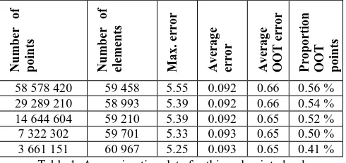
The original data set contains 58 578 420 points. We approximate this with a tolerance of 0.5 m and maximum number of iteration levels 6. The quality of the output approximation can be seen in the first row of Table 1. In particular, the proportion of points that are out-of-tolerance (OOT) after six iterations is approximately 0.56%.
In each row of the table, we successively thin the point cloud and approximate with LR B-spline surfaces of the same tolerance and number of levels (0.5 m and 6 levels). It can be seen that the resulting numbers are fairly constant. The proportion of OOT points reduces very slightly with thinning until the point cloud is thinned to 1/16th of its original size, at which point, significant details begin to be lost.
There are some subtleties in the refinement algorithms that mean that in this example more refinements are added with fewer points. However, this does not affect the significance of the results. This example demonstrates that the resulting data size of LR B-spline approximations has more relation to the topographic features of the data set than the density of the input points.
4.2 Example 2: Liguria
This second example considers topographic data from Liguria, Italy, courtesy Regione Liguria and CNR-IMATI. The data set contains 3 045 671 points. The region covered by the data is dominated by mountainous terrain and sharp features such as buildings. Although spline representations are typically best suited to modelling smooth data, our algorithms are capable of providing an approximate representation of the underlying terrain that can be used to classify points according to their distance from the surface. In this example we use a tolerance of 0.5 m, and stop the iteration after six levels. This avoids the surface picking up the finer details by restricting the number of refinements, but provides sufficient accuracy to show the trends of the underlying terrain.
Figure 2: LR B-spline approximation of Liguria dataset and the point classification coloured according to the distance from the surface approximation. White points lie close to the surface, whereas green points lie below the surface tolerance level and
red points above.
The resulting surface contains 85 206 coefficients with 2 453 333 points out-of-tolerance. The average distance between the points and the surface is 2.6 m and the maximum distance is 88.9 m. Though the maximum may seem large, it is caused by a outliers that are positioned high above the other surface points.
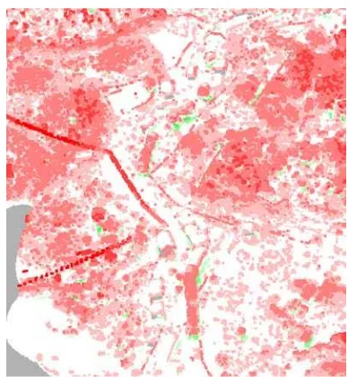
In Figure 2 the surface approximation is pictured together with a classification of the points according to their distance from the surface. It is worth remarking that this point classification could potentially be a useful tool for feature detection. For example, as can be seen by the close-up view of the classified points in Figure 3, features such as building footprints can be distinguished. This could be useful for automating the extraction of building features, especially in the absence of supporting cadastral data. However, to what degree building footprint extraction and can be automated via our approach, and
to what level of accuracy, is subject for future research. Typically when processing geospatial data, the amount of user input required for reconstructing building models increases with the level of detail required (Tack et al., 2012). Thus, any tools to support automation could be useful in a big data context. Vegetation and other objects such as electricity cables are also highlighted by the point classification method.
Figure 3: Close-up view of the classified Liguria point set using the surface from Figure 2(a). Features of the data set can clearly
be distinguished.
As the classification of points in this example utilizes the lower quality surface approximations, the removal of features that do not belong to the terrain surface can be performed dynamically in the algorithm. Points that are not part of the underlying surface can be filtered and passed to other algorithms for processing (e.g., as building triangulations or vegetation), whilst the remaining terrain points can be included in higher level surface approximations. Such a workflow could provide the basis for an automated algorithm for a hybrid solution, as discussed in Section 182.5.
4.3 Example 3: HRW Bathymetric data set containing several surveys
0.5 7 142237 0.09 7.10 165596 9.8 0.5 8 323012 0.08 6.40 81587 24.0 0.25 6 58112 0.13 9.01 1264136 4.0 0.25 7 147612 0.09 7.33 615763 11.0 0.25 8 369438 0.07 7.22 355006 27.0 Table 2: Results of LR B-spline surface approximations of the
combined bathymetry data set (Figure 4) for various input tolerances and iteration levels
Figure 4: An LR B-spline surface approximation of the HRW combined bathymetry data set with tolerance 0.5 m and
maximum iteration levels six.
As can be seen from the results in Table 2, reducing the tolerance has most effect on the average error. It results in more refinements at each approximation level so that the resulting number of coefficients is also increased. The maximum error is reduced by allowing the approximation algorithm to continue to higher levels of refinement; however when outliers are present, the maximum error will remain high unless very high iteration levels are chosen. Generally, the higher the chosen iteration level, the more detailed are the features included in the surface approximation.
It may be noted that for the smaller tolerances, the amount of data in the resulting surface approximately doubles. This indicates that there are many local regions with points that lie out-of-tolerance. However, depending on the accuracy of the original data and the characteristics of the terrain, it may not always be necessary to model with such small tolerances.
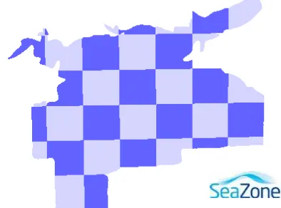
The number of iteration levels chosen should also reflect the extent of the region to be modelled. If a large region is to be modelled, higher levels of refinement are required to achieve a given accuracy than if the region is relatively small. In cases where the region is so large that a very high approximation level would be required to model the surface to a given accuracy, tiling may be appropriate. This involves splitting the data into regular patches and approximating each patch separately. This can be followed by a post processing step that ensures the patches connect with the required degree of continuity given by the degree of the spline representation. An example of tiled approximation is shown in Figure 5. Tiling allows the size of each surface patch to remain relatively small, but will result in increased amounts of data across patch boundaries.
In future research we will consider to what extent the choice of the approximation parameters can be automated based on the characteristics of the input data.
Figure 5: An example of the pattern of a tiled approximation where each tile represents one surface.
ACKNOWLEDGEMENTS
The results presented in this paper are results of the research in the IQmulus project. The IQmulus project has received funding from the European Union’s Seventh Framework Programme under grant agreement No 318787. We would like to thank HR Wallingford, Regione Liguria and CNR-IMATI for providing access to the data sets used in the examples.
REFERENCES
De Floriani, L., Paola M., and Enrico P.. "Compressing triangulated irregular networks." Geoinformatica 4.1 (2000), pp 67-88.
Dokken T., Lyche T., and Pettersen K.F., Polynomial splines over locally refined box-partitions, Computer Aided Geometric Design, 30(2013), pp 331–356.
Forsey D.R., and Barrels R.H., Hierarchical B-Spline Refinement, Comput. Graphics, 22(1988), pp. 205-212.
Giannelli C., Jüttler B., and Speleers H., THB-splines: the truncated basis for hierarchical splines. Computer Aided Geometric Design, 29(2012), pp. 485-498.
Hughes T.J.R., Cottrell J.A., and Bazilevs Y., Isogeometric analysis: CAD, finite elements, NURBS, exact geometry, and mesh refinement, Comput. Methods Appl. Mech. Engrg., 194(2005), pp. 4135--4195.
Kraft R., Adaptive und linear unabhangige multilevel B-splines und ihreAnwendungen, PhD thesis, Math Inst A, University of Stuttgart, Germany, 1998.
Pfeifer, N. "A subdivision algorithm for smooth 3D terrain models." ISPRS journal of photogrammetry and remote sensing 59.3(2005), pp. 115-127.
Sederberg T.W., Zheng J., Bakenov A., and Nasri A., T-splines and TNURCCS, ACM Transactions on Graphics (TOG), ACM Trans. Graph.,22 (2003), pp. 477-484.
Sulebak J.R, and Hjelle Ø., Multiresolution Spline Models and Their Applications in Geomorphology, in Concepts and Modelling in Geomorphology: International Perspectives, Eds. Evans I. S., Dikau R., Tokunaga E., Ohmori H., and Hirano M., TERRAPUB, Tokyo, Japan, 2003, pp. 221–237.