ORIENTATION AND CALIBRATION REQUIREMENTS FOR HYPERPECTRAL IMAGING USING UAVs: A CASE STUDY
A. M. G. Tommaselli a *, A. Berveglieri a, R. A. Oliveira a, L. Y. Nagai a, E. Honkavaara b
a Univ Estadual Paulista, Unesp, Brazil - [email protected] [email protected], [email protected], [email protected]
Finnish Geospatial Research Institute FGI, Kirkkonummi, Finland - [email protected]
Commission I, ICWG I/Va
KEY WORDS: Geometric Calibration; Hyperspectral frame cameras; two sensors camera
ABSTRACT:
Flexible tools for photogrammetry and remote sensing using unmanned airborne vehicles (UAVs) have been attractive topics of research and development. The lightweight hyperspectral camera based on a Fabry-Pérot interferometer (FPI) is one of the highly interesting tools for UAV based remote sensing for environmental and agricultural applications. The camera used in this study acquires images from different wavelengths by changing the FPI gap and using two CMOS sensors. Due to the acquisition principle of this camera, the interior orientation parameters (IOP) of the spectral bands can vary for each band and sensor and changing the configuration also would change these sets of parameters posing an operational problem when several bands configurations are being used. The objective of this study is to assess the impact of use IOPs estimated for some bands in one configuration for other bands of different configuration the FPI camera, considering different IOP and EOP constraints. The experiments were performed with two FPI-hyperspectral camera data sets: the first were collected 3D terrestrial close-range calibration field and the second onboard of an UAV in a parking area in the interior of São Paulo State.
1. INTRODUCTION
Environmental mapping and monitoring of forest areas have been greatly facilitated with the use of Unmanned Aerial Vehicles (UAV) carrying imaging sensors, like hyperspectral cameras. Higher temporal and spatial resolution can be achieved when using UAVs making feasible several detailed analysis that are more complex to achieve with existing remote sensing sensors. Recently, hyperspectral cameras have been adapted for UAV platforms, which are lightweight and some of them acquiring frame-format images (Saari et al., 2009; Honkavaara et al., 2013; Aasen et al., 2015; Näsi et al., 2015). Existing pushbroom based hyperspectral cameras require high grade Inertial Navigation Systems (INS) to provide instantaneous position and attitude and this type of systems are high cost and sometimes heavy. Frame format hyperspectral cameras are attractive alternatives because bundle adjustment can be used to compute platform attitude and position, relaxing the need for high grade IMU, stereo reconstruction is feasible and multidirectional reflectivity features can be measured (Honkavaara et al., 2013).
One example of frame based hyperspectral cameras is the Rikola camera (Rikola Ltd., 2015), which acquires a sequence of images in different spectral bands, with frame geometry. This camera uses a technology based on a tuneable Fabry-Perot Interferometer (FPI), which is placed into the lens system to collimate the light that transmits the spectral bands as a function of the interferometer air gap (Saari et al., 2009). Using several air gap values of the FPI, a set of wavelengths is acquired enabling capture of hyperspectral frame format imagery at desired spectral bands.
Estimating Exterior Orientation Parameters (EOPs), describing platform position and attitude is fundamental when accurate 3D information is required, which has been more common in several environmental applications. EOPs can be determined directly, by using INS, indirectly, by Bundle Adjustment on by Integrated Sensor Orientation (ISO) which is a combined strategy. In any case, rigorous sensor modelling
is required. The most common sensor model in Photogrammetry uses a set of Interior Orientation Parameters (IOPs) to recover the optical path within the sensor. The IOPs must be accurately determined by camera calibration, which can be done by laboratory or field techniques. However, it cannot be ensured that the IOPs determined by laboratory or terrestrial techniques are stable, because of the camera operational characteristics and the hard environmental conditions, with vibrations, impacts and temperature variations. In such a case of IOPs variations, the results of BBA or ISO are likely to be affected. For this reason, it is relevant to assess the behaviour of these new cameras when doing this combined process (terrestrial calibration followed by aerial survey and BBA). Also, as this camera is reconfigurable, the set of bands can be changed depending on the reflectance properties of the objects to be sensed. This poses an additional and critical problem since it is unfeasible to generate IOPs for all possible sets of configurations that can be tested and used in a surveying.
The main aim of this paper is to present an experimental assessment of the bundle block adjustment (BBA) and on-the job calibration (OJC) performed with different spectral bands of the hyperspectral frame camera (Rikola), using IOPs estimated by close range terrestrial calibration. For both cases different sets of IOPs and EOPs constraints were considered and assessed. This study can drive future effort to set some requirements for the calibration and orientation of cameras with similar features. The importance of the assessment of these different configurations is related with the future use of the UAV-FPI camera in forest areas, where the access to the inside area limits the collection of control points.
2. BACKGROUND 2.1 Hyperspectral cameras
Hyperspectral cameras can grab up to hundreds of spectral bands and, from this data, the reflectance spectrum of each image pixel can be reconstructed. Usually these cameras were
based on pushbroom or whiskbroom scanning (Schowengerdt, 2007).
Alternatives are hyperspectral cameras which grab two-dimensional frame format images based on tuneable filters (Saari et al., 2009; Lapray et al., 2014; Aasen et al., 2015). Some of these cameras acquire the image cube as a time dependent image sequence (Honkavaara et al., 2013) whilst others grab the entire cube at the same time, but at the cost of having low resolution images (Aasen et al., 2015). The unsynchronised cameras require a post-processing registration step to produce a coregistered hyperspectral image cube.
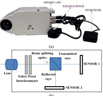
Some of these cameras are of particular interest for applications requiring high resolution (temporal, spectral and spatial)because they are lightweight and thus can be carried by UAVs. One of these lightweight hyperspectral camera based on a Fabry-Pérot Interferometer (FPI), was developed by the VTT Technical Research Centre of Finland (Saari et al., 2009). Rikola Ltd. (2015) manufactures cameras based on this technology for the commercial market and one of these cameras was used in this work. A summary of technical specifications can be seen in Table 1 and a picture of the camera and components are shown in Fig. 1.a. The camera has several internal components and the most important one is a FPI which has two partially reflective parallel plates with variable distance (air gap) which is controlled by piezoelectric actuators (Saari et al., 2009). The wavelengths transmitted Spectral Resolution 10 nm (FWHM)*
F-number ~2,8
Sensors CMOS - CMV400
Images dimensions 1023 x 648 pixels Pixel size 5.5 μm x 5.5 μm Principal distance 8.7 mm
Weight ~ 700 g
*FWHM – Full Width at Half Maximum Source: Adapted from Rikola Ltd. (2016). Table 1. Specifications of a Rikola camera, model 2014.
Figure 1.a shows the 2014 model with external components: irradiance sensor and a GPS receiver of a Rikola camera. The rays bundle passes through the primary lens and other internal optical components, including the FPI and is redirected to two CMOS sensors by a beam splitting device (Fig. 1.b). Sensor 1 receives energy from near infrared (650–900 nm) and Sensor 2 is optimised to record bands of the visible part of the spectrum (500–636 nm). The spectral bands and their range limits can be selected by the user, depending on the application. Due to these features, it is unfeasible to define a single set of IOPs for this camera and alternatives have to be derived. Deriving a set of IOPs for each image band is troublesome because the configuration can change depending on the application. On the other side, a single set of IOPs for each sensor or for both sensors is also unsuitable to cope with the sensors misalignments and eventual changes in the IOPs due to the internal changes in the rays paths. Depending on
Figure 1. (a) Rikola Hyperspectral camera with accessories and (b) diagram showing internal components.
2.2 Bundle Adjustment and camera calibration
Bundle adjustment is a standard photogrammetric technique for determination of sensor orientation that can also be used to estimate the parameters of the internal sensor model (Brown, 1971; Clarke and Fryer, 1998; Remondino and Fraser, 2006). The camera IOPs are usually the principal distance, principal point coordinates, lens distortions and affinity coefficients (Brown, 1971; Habib and Morgan, 2002).
The well-known collinearity equations are used as the main mathematical model, as can be seen in Eq. 1.
) are the ground coordinates of the corresponding point; mij are the elements of the rotation matrix; X0, Y0 and Z0 are the ground coordinates of the camera’s perspective centre (PC); x0 and y0are the coordinates of the principal point; c is the camera’s principal distance; δxi and δyi are the effects of radial and decentring distortions and affinity.
The IOPs, EOPs and the ground coordinates of tie points can be estimated simultaneously, using the image coordinates of the these points and additional observations, such as the ground coordinates of some points, coordinates of the PC, determined by GNSS. Another technique, known as self calibration (Kenefick et al., 1972; Merchant, 1979) does not use control points (GCPs), but a set of minimum of seven constraints to define an object’s reference frame (Kenefick et al., 1972; Merchant, 1979), avoiding the error propagation of the GCP surveying. The frame definition can be done by constraining the six EOPs of one selected image and one or more distances (Kenefick et al., 1972).
3. METHODOLOGY AND EXPERIMENTS There are several differences between FPI cameras and conventional digital photogrammetric cameras. In the FPI camera system, the set of bands can be selected according to the target spectra responses and application. Thus, a formal camera calibration certificate is unfeasible to be used in the photogrammetric data processing. In the current study, the objects are trees from tropical forest and their reflectance factors can be estimated by field or laboratory measurements.
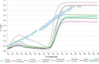
3.1 Selecting bands configurations for forest coverage Selection of the spectral bands to be used in the Rikola camera were based on measurement performed over tree leafs of one selected area over the tropical forest. Leaves were collected in the study area and stored in proper boxes. Radiometric measurements were performed in laboratory with a spectroradiometer (Specfield hand held Pro – ASD) six hours after the field collection. The species collected are: Pouteria ramiflora; Croton floribundus; Astronium graveolens; Aspidosperma ramiflorum; Handroanthus avellanedae; Hymenaea courbaril and Eugenia uniflora. The CCRF (Conical Conical Reflectance Factor) were obtained and the spectral range was limited to 500 nm e 900 nm, corresponding to the Rikola capability. Figure 2 presents the CCRF curves extracted for some leaf samples. It can be observed that changes in the curve intensities occurred mainly in the near infrared and yellow spectral bands. The spectral features of those species are useful for future hyperspectral classification (Miyoshi, 2016).
Figure 2. CCRF curves of leafs and selected spectral bands (Adapted from Miyoshi, 2016).
The spectral bands configuration were defined by using the main differences on the CCRF curves, the wavelengths of some vegetation indexes (REP, SR, NDVI) bounded by some restrictions of the Rikola camera. Two configurations with 25 bands were defined to be tested. Their features (band number, central wavelength and FWHM) are shown in Tables 2 and 3. As it can be seen the wavelengths of the two configurations are similar but do not match, which means that the IOPs for each different configuration may be different.
In this work the terrestrial calibration was performed with configuration 2 (Table 2) and the camera was reconfigured to configuration 1 (Table 1) for the flight, simulating scenarios of real projects. The main question is whether the IOPs derived for configuration 2 could be used for configuration 1 and what should be the results with some refinement with on-the-job calibration.
Band
id λ (nm) FWHM (nm) Band λ (nm) FWHM (nm) 1 506.07 15.65 14 680.06 21.00 2 520.00 17.51 15 689.56 21.67 3 535.45 16.41 16 699.62 21.89 4 550.76 15.16 17 709.71 20.78 5 564.71 16.60 18 719.99 20.76 6 580.08 15.14 19 729.56 21.44 7 591.49 14.67 20 740.45 20.64 8 605.64 13.82 21 749.65 19.43 9 619.55 14.59 22 770.46 19.39 10 629.93 22.85 23 790.21 18.50 11 650.28 15.85 24 810.15 17.66 12 660.27 24.11 25 829.93 18.62 13 669.96 21.70
Table 2. Spectral configuration 2 used in the terrestrial calibration (cfg. 2).
Band λ (nm) FWHM (nm) Band λ (nm) FWHM (nm) 1 506.07 15.65 14 680.06 21.00 2 520.00 17.51 15 689.56 21.67 3 535.45 16.41 16 699.62 21.89 4 550.16 15.18 17 709.71 20.78 5 564.71 16.60 18 719.99 20.76 6 580.08 15.14 19 729.56 21.44 7 592.78 14.81 20 740.45 20.64 8 609.79 13.77 21 749.65 19.43 9 619.55 14.59 22 770.46 19.39 10 629.23 12.84 23 780.16 18.25 11 650.28 15.85 24 790.21 18.50 12 660.27 24.11 25 819.70 18.17 13 669.96 21.70
Table 3. Spectral configuration 1 used in flight (cfg. 1).
3.2 Terrestrial camera calibration
The first step is the estimation of the camera IOPs by self-calibrating bundle adjustment, using images acquired in a 3D terrestrial calibration field composed of coded targets with the ArUco codification (Garrido-Jurado et al., 2014; Tommaselli et al., 2014). Each target is composed of a rectangular external crown and 5 x 5 internal squares arranged in five rows and five columns (see Figure 3). The automatic processing for locating, identifying and accurately measuring the corners of the crown has been described by Tommaselli et al. (2014).
In this camera model, two CMOS sensors were used. To cope with this geometry, the calibration was made for both sensors using a reference spectral band for each sensor. Firstly, the camera was configured with the cfg. 2 (Table 2) and calibrated considering two reference bands for each sensor (band 8 for sensor 2 and band 23 for sensor 1). Then, additional calibrations trials were performed for more two bands of the sensor 1 (bands 15 and 22). Twelve cubes were acquired with different positions and rotations (Table 4). The reference frame for the self-calibration with bundle adjustment was defined by the 3D coordinates of two points and the Z coordinate (depth) of a third point. The first point was set as the origin of the system. The distance between the two points was measured with a precision calliper and the Y and Z coordinate of this second point were the same as the first point.
(a)
(b)
Figure 3. (a) Set of twelve images of band 8 (605.64 nm) used for calibration; (b) example of corners automatically extracted
and labelled.
Sensor 2 1
Band id. 8 15 22 23
λ (nm) 605.64 689.56 770.46 790.21
Number of images 12 12 12 12
Num. of image points 572 584 568 572
Ground Points 84 80 80 80
Table 4. Image bands used for terrestrial calibration and the number of images and points.
The IOPs, the EOPs and the object coordinates of the tie points were simultaneously estimated in the adjustment based only on internal information (7 constraints), except the distance measured in the object space. The self-calibration adjustment was performed using an in-house-developed software Calibration with Multiple Cameras (CMC) (Tommaselli et al., 2013), which uses the unified approach for least-squares (Mikhail and Ackermann, 1976, p. 133).
The standard deviations of the image observations were considered to be 0.5 pixels for x and y coordinates and the a priori variance factor was set to 1. The full set of ten parameters was firstly used in the calibration experiments, but the effects of affine parameters were deemed to be insignificant and were removed. The experiments were then performed with 8 parameters (c, x0, y0, k1, k2, k3, P1, P2). In some cases k3 was not significant but it was used to maintain the same configuration.
Table 5 presents the a posteriori sigma for image bands of sensors 1 and 2, the estimated IOPs and corresponding standard deviations of estimated values. It is clear that the results achieved for sensor 1 are better than for sensor 2. This can be explained by the image quality: images from sensor 2 are more blurred probably due to the beam splitting optics. The values for the parameters are clearly different for images from different sensors. When comparing the results for bands of sensor 1 (15, 22 and 23) it clear that they are similar and the differences are within the estimated standard deviations.
Sensor 2 1
Band id. 8 15 22 23
A posteriori
Sigma 0.65 0.25 0.33 0.33
c
(mm) ± 0.032 8.648 ± 0.011 8.690 ±0.0163 8.6949 ±0.0163 8.7000 x0
(mm) ± 0.013 0.366 ± 0.005 0.416 ±0.0070 0.4073 ±0.0070 0.4084 y0
(mm) ± 0.010 0.436 ± 0.003 0.399 ±0.0054 0.4024 ±0.0054 0.4006 K1
(mm-2) ±0.00030 -0.00412 ± 0.00010 -0.00473 ±0.00014 0.00460 ±0.00014 -0.00452 K2
(mm-4) ±6.5 E-05 -6.3 E-05 ±2.2 E-05 -1.7 E-06 ±3.1 E-05 -3.2 E-06 ±3.1 E-05 -5.2 E-05 K3
(mm-6) ±4.3 E-06 4.7 E-06 ±1.4 E-06 -6.7 E-07 ±2.0 E-06 7.0 E-07 ±2.0 E-06 2.3 E-06 P1
(mm-1) ±2.4 E-05 -1.7 E-04 ±8.8 E-06 -2.8 E-05 ±1.2 E-05 -4.9 E-05 ±1.2 E-05 -3.9 E-05 P2
(mm-1) ±3.1 E-05 -3.0 E-04 ±1.1 E-05 -1.1 E-04 ±1.6 E-05 -1.2 E-04 ±1.6 E-05 -1.0 E-04 Table 5. Estimated IOP and a posteriori sigma for image
bands of sensors 1 and 2.
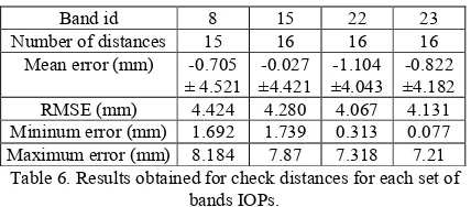
The quality control of the calibration results were based on the analysis of the a posteriori sigma, the estimated standard deviation of the IOPs and also the discrepancies of check distances. These distances were measured directly in the field with a calliper and the corresponding distances were computed using the coordinates estimated in the bundle adjustment. Table 6 presents the results showing that the RMSE for the check distances were around 4.4 mm for band 8 (Sensor 2) and 4.2 mm for bands of Sensor 1. This value is expected since the average pixel footprint is around 4 mm.
Band id 8 15 22 23
Number of distances 15 16 16 16
Mean error (mm) -0.705
± 4.521 ±4.421 -0.027 ±4.043 -1.104 ±4.182 -0.822 RMSE (mm) 4.424 4.280 4.067 4.131 Mininum error (mm) 1.692 1.739 0.313 0.077 Maximum error (mm) 8.184 7.87 7.318 7.21 Table 6. Results obtained for check distances for each set of
bands IOPs.
In order to compare the equivalence of the estimated sets of IOPs for several image bands, the ZROT (Zero Rotation Method) developed by Habib and Morgan (2006) was used. First, a regular grid is defined in the image space. The two sets of IOPs to be compared are used to refine the coordinates of each grid point, thus removing distortions. The differences in the principal distances are compensated by projecting the coordinates of the second set to the image plane of the first set. The RMSE of these two grid points are computed and can be used to assess the similarity of the bundles generated with these grid points and the two sets of IOPs. If the differences were within the expected standard deviation of the image coordinate measurements, then the IOP set could be considered to be equivalent (Habib and Morgan, 2006).
Table 7 presents the results of the ZROT method for three pairs of sets of IOPs: the first pair compares IOPs generated with images of band 8 (Sensor 2) with those IOPs generated for the band 23 (Sensor 1) and the other two pairs compare bands of the same sensor (bands 15 and 22 of sensor 1).
IOPs sets 8-23 15-23 22-23 RMSEx (μm) 45.541 9.583 1.763 RMSEy (μm) 36.958 1.650 2.314 Table 7. Results of ZROT method comparing sets of pairs of
sets of IOPs.
It can be seen that the RMSEx and RMSEy were smaller than half pixel for the IOPs generated with images of bands from the same sensor, except for the RMSEx of band 15. However, the IOPs from different sensors presented RMSEs higher than 8 pixels, and can be considered different, as also was observed from the analysis of Table 5.
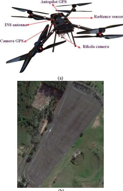
3.3 Validation with images collected from an UAV An UAV octopter (Fig. 4.a) was equipped with the hyperspectral camera and a dual-frequency GNSS receiver (Novatel SPAN-IGM) to acquire a set of aerial images in a nearly flat test field (parking area, see Fig. 4.b). The camera was configured with the spectral set cfg. 1 (Table 3) which is slightly different from the cfg. 2, used in the terrestrial calibration, with an integration time of 5 ms.
(a)
(b)
Figure 4. (a) UAV with camera and accessories; (b) Parking area used in the experiments (source: Google Earth).
An image block (composed of two flight strips) with a range of approximately 360 m was collected at a flight height of 90 m, which generated spectral images with 25 bands and GSD of 6 cm. Forward overlap was approximately 60% and side overlap varied from 10 to 20 %. Nineteen ground points
arranged in the block were surveyed with double frequency GNSS receivers and six were used as control and other thirteen as check points. Two bands of cfg. 1 were selected for this empirical assessment: band 8 (609.79 nm, Sensor 2) and band 23 (786.16, Sensor 1) which do not correspond with those with the same id for the calibration set in which cfg. 2 was used.
GPS time for each event of cube acquisition (intervals of 4 s) was grabbed by the Rikola GPS receiver. This time refers to the first cube band and the acquisition time of the remaining bands were estimated by the nominal time differences (22 ms). A spreadsheet (SequenceInfoTool), supplied by Rikola, was used to perform this estimation from the metadata files and the GPS log file stored for each cube. The double frequency GNSS receiver of the Novatel SPAN-IGM-S1 grabbed raw data with a frequency of 1 Hz and from this data accurate positions were computed. A reference station was settled in the area and a double frequency receiver collected data during the flight. The trajectory was computed with differential positioning technique with Inertial Explorer Software achieving standard deviations of 2 cm for horizontal and vertical components. The position of each image band was interpolated from these data and used as observations in the bundle adjustment with a standard deviation of 20 cm for XYZ coordinates. Antenna to camera offsets were directly measured and used in the trajectory processing. The attitude angles provided by the INS were not used in the experiments.
Two photogrammetric projects were set up for each set of images from bands 8 and 23 to perform the BBA with Leica Photogrammetric Suite (LPS). The Perspective Centre coordinates determined by GPS were used as weighted constraints and the attitude angles were considered as unknowns. Tie points were automatically extracted with Leica LPS software.
Figure 5. Block configuration used in the experiments. Several trials were conducted using bundle block adjustment (BBA) to assess the suitability of the previously determined IOPs in the indirect image orientation considering three settings: the first one used the calibrated IOPs as fixed and the EOPs as unknowns; the second trial used fixed IOPs and weighted constraints in the EOPs to perform bundle adjustment and; the third trial used and weighted constraints in the IOPs and in the EOPs to perform on-the-job calibration. Several variations in the weights of the PC coordinates and IOPs were also performed to check the results because there is some uncertainty about the accuracy of the
technique used for event synchronization with two different receivers (single frequency used by Rikola and dual frequency used by Novatel). Event logging directly from the Rikola to SPAN-IGM is planned to be implemented in the near future to provide more accurate event handling.
In this paper only the most significant results will be presented. Tables 8 and 9 to 11 present the a posteriori sigma and the RMSE in the check points for the experiments with images of band 8 and 23, respectively. These results were obtained with LPS Aerial Triangulation module and checked with CMC, which achieved similar values.
In Table 8, column two refers to results with BBA without constraints in the EOPs (considered as unknowns) and IOP fixed; column three shows results when imposing constraints in PC coordinates with standard deviations of 20 cm for XYZ and IOP fixed. In both cases IOPs used were those generated by terrestrial calibration for band 8 with cfg. 2, which central wavelength is slightly different (see Tables 2 and 3; 605.64 nm for cfg. 2 and 609.79 nm for cfg. 1). Column 4 shows the results when the IOPs (c, xo, yo) were left to vary with σ=15 µm, a value which corresponds to approximately three pixels (On-the-Job Calibration OJC)
BBA 1 BBA 2 OJC
σ
IOP(c, xo, yo) fixed fixed 15 µmσ
PC(m)
unknown- 0.2 0.2A posteriori σ 0.386 0.638 0.441
RMSE X (m) 0.246 0.281 0.217
RMSE Y (m) 0.259 0.423 0.266
RMSE Z (m) 0.469 1.232 0.562
Table 8. Results for aerial images of band 8 with IOPs of band 8 from terrestrial calibration: a posteriori sigma and
RMSE in the check points coordinates.
Comparing the estimated PC coordinates of the BBA_1 with those grabbed by GPS, systematic differences of more than 1.5 meters in XYZ were observed which could be caused by delays in event logging or systematic errors in the IOPs. The second experiment (BBA 2), in which constraints were imposed to PC coordinates, produced large errors in the Z component of check points and in the a posteriori sigma. Then, IOPs (c, xo, yo) were treated as weighted constraints and the results improved (both the RMSE of Z and a posteriori sigma). More experiments were conducted with different weights and similar results were achieved.
Similar experiments were performed using the band 23 of cfg. 1 and IOPs generated by terrestrial calibration for band 23 with cfg. 2 (central wavelengths were 780.16 nm and 790.21 nm; see Tables 2 and 3). The configuration of the constraints in the EOPs and IOPs were the same as presented for band 8. The results are presented in Table 9.
BBA 1 BBA 2 OJC
σ
IOP(c, xo, yo) fixed fixed 15 µmσ
PC(m)
unknown- 0.2 0.2A posteriori σ 0.446 0.721 0.505
RMSE X (m) 0.259 0.290 0.236
RMSE Y (m) 0.191 0.150 0.129
RMSE Z (m) 0.650 0.930 0.524
Table 9. Results for aerial images of band 23 with IOPs of band 23 from terrestrial calibration: a posteriori sigma and
RMSE in the check points coordinates.
The results with images of band 23 were similar to band 8, showing that small corrections in the IOPs are required to improve results. The experiment was repeated but changing the initial IOPs for those obtained for band 22 and 15 with terrestrial calibrations. Results are presented in Tables 10 and 11, showing similar results.
BBA 1 BBA 2 OJC
σ
IOP(c, xo, yo) fixed fixed 15 µmσ
PC(m)
unknown- 0.2 0.2A posteriori σ 0.449 0.734 0.509
RMSE X (m) 0.261 0.293 0.238
RMSE Y (m) 0.194 0.154 0.129
RMSE Z (m) 0.639 0.967 0.527
Table 10. Results for aerial images of band 23 with IOPs of band 22 from terrestrial calibration: a posteriori sigma and
RMSE in the check points coordinates. .
BBA 1 BBA 2 OJC
σ
IOP(c, xo, yo) fixed fixed 15 µmσ
PC(m)
unknown- 0.2 0.2A posteriori σ 0.445 0.727 0.506
RMSE X (m) 0.260 0.290 0.235
RMSE Y (m) 0.191 0.154 0.129
RMSE Z (m) 0.674 0.994 0.530
Table 11. Results for aerial images of band 23 with IOPs of band 15 from terrestrial calibration: a posteriori sigma and
RMSE in the check points coordinates.
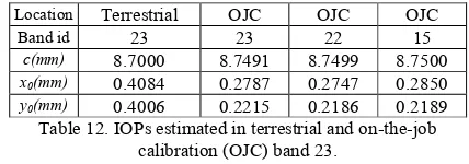
A further analysis was performed comparing the IOPs (c, xo, yo) estimated with on-the-job calibration with aerial images of band 23 and using initial values provided by terrestrial calibration with images from bands 23, 22 and 15. The estimated values are presented in Table 12. It can be seem that the IOPs estimated on-the-job have similar values, no matter the initial values used and these values are different from those obtained in the terrestrial calibration, specially the coordinates of the principal point. This can be explained by the mechanical instability or even to delay in the event logging which can be absorbed by the estimated coordinates of the principal point.
Location Terrestrial OJC OJC OJC
Band id 23 23 22 15
c(mm) 8.7000 8.7491 8.7499 8.7500
x0(mm) 0.4084 0.2787 0.2747 0.2850
y0(mm) 0.4006 0.2215 0.2186 0.2189
Table 12. IOPs estimated in terrestrial and on-the-job calibration (OJC) band 23.
It can be concluded that for medium accuracy the conventional BBA leads to suitable results. For areas with difficult terrestrial access, such as forest areas, direct georeferencing is recommended and, then, OJC should be required to compensate these variations in the IOPs.
4. CONCLUSIONS
The aim of this study was to assess the use of a lightweight hyperspectral camera based on a Fabry-Pérot interferometer (FPI) with photogrammetric techniques. The main concern when using this FPI camera is the determination of the IOPs and its change with different bands configurations. Experiments with some reference bands of two sensors were performed both with terrestrial and aerial data.
The configurations were not optimal, mainly the side overlap. Also, only one flight height was used and it should be better to use two flights heights to minimize correlations. The results have shown that some IOPs have to be estimated on-the-job with bundle adjustment to provide suitable results, especially when using direct georeferencing data. Combining GNSS data is of crucial importance in forest applications because of the difficult to establish dense control in the block extent. Further research is needed to assess the stability of the camera inner orientation and the use of IOP values of some reference bands.
ACKNOWLEDGEMENTS
The authors would like to acknowledge the support of FAPESP (Fundação de Amparo à Pesquisa do Estado de São Paulo - grant 2013/50426-4), CNPq (Conselho Nacional de Desenvolvimento Científico e Tecnológico - grant 307554/2014-7) and Academy of Finland (Decision number 273806). The authors are also thankful to Gabriela T. Miyoshi, Fernanda Torres and Lucas D. Santos who helped in data collection and some experiments.
REFERENCES
Aasen, H., Burkart, A., Bolten, A., Bareth, G, 2015. Generating 3D hyperspectral information with lightweight UAV snapshot cameras for vegetation monitoring: from camera calibration to quality assurance. ISPRS Journal of Photogrammetry and Remote Sensing, 108, pp.245-259. Brown, D. C., 1971. Close-Range Camera Calibration, Photogrammetric Engineering, 37(8): pp.855-866.
Clarke, T.A., Fryer, J.G., 1998. The Development of Camera Calibration Methods and Models, Photogrammetric Record, 16(91), pp. 51–66.
Garrido-Jurado, S., Muñoz-Salinas, R., Madrid-Cuevas, F. J., Marín-Jiménez, M. J., 2014. Automatic generation and detection of highly reliable fiducial markers under oclusion. Pattern Recognition, 47(6), pp. 2280-2292.
Habib, A.F., Morgan, M., Lee, Y., 2002. Bundle Adjustment with Self–Calibration Using Straight Lines. Photogrammetric Record, 17(100), pp. 635-650.
Habib, A., Pullivelli, A., Mitishita, E., Ghanma, M., Kim, E. M., 2006. Stability analysis of low-cost digital cameras for aerial mapping using different georeferencing techniques. Photogrammetric Record, 21(113), pp. 29-43.
Hagen, N., Kudenov, M. W., 2013. Review of snapshot spectral imaging technologies. Optical Engineering, 52(9), pp. 090901-090901.
Honkavaara, E., Saari, H., Kaivosoja, J., Pölönen, I., Hakala, T., Litkey, P., Mäkynen, J., Pesonen, L., 2013. Processing and Assessment of Spectrometric, Stereoscopic Imagery Collected Using a Lightweight UAV Spectral Camera for Precision Agriculture. Remote Sensing, 5(10), pp. 5006-5039.
Kenefick, J. F., Gyer, M. S., Harp, B. F., 1972. Analytical Self-Calibration. Photogrammetric Engineering, 38, 1117-1126.
Lapray, P. J., Wang, X., Thomas, J. B., Gouton, P., 2014. Multispectral filter arrays: Recent advances and practical
implementation. Sensors, 14(11), pp. 21626-21659.
Mäkynen, J., Holmlund, C., Saari, H., Ojala, K., Antila, T., 2011. Unmanned Aerial Vehicle (UAV) operated megapixel spectral camera. Proceedings of SPIE, Electro-Optical Remote Sensing, Photonic Technologies, and Applications V, 8186, pp. 81860Y-1–81860Y-9.
Mäkynen, J. A., 2009. Lightweight Hyperspectral Imager, 2009. 74f. Master's Thesis, Helsinki University of Technology, Helsinki, Finland. 74 pages. http://lib.tkk.fi/Dipl/2009/urn100105.pdf
Mäkeläinen, A., Saari, H., Hippi, I., Sarkeala, J., Soukkamaki, J., 2013. 2D Hyperspectral frame imager camera data in photogrammetric mosaicking. International Archives of the Photogrammetry, Remote Sensing and Spatial Information Sciences, XL-1/W2, pp. 2-267.
Merchant, D. C., 1979. Analytical Photogrammetry: Theory and Practice. Notes Revised from Earlier Edition Printed in 1973, Ohio State University: Columbus, USA.
Miyoshi, G. T. 2016. Caracterização espectral de espécies de Mata Atlântica de Interior em nível foliar e de dossel. 125 p. MSc. dissertation, Presidente Prudente, SP, 2016. (In Portuguese)
Näsi, R., Honkavaara, E., Lyytikäinen-Saarenmaa, P., Blomqvist, M., Litkey, P., Hakala, T., Viljanen, N., Kantola, T., Tanhuanpää, T., Holopainen, M., 2015. Using UAV-based photogrammetry and hyperspectral imaging for mapping bark beetle damage at tree-level. Remote Sensing, 7(11), pp. 15467-15493.
Remondino, F., Fraser, C., 2006. Digital camera calibration methods: considerations and comparisons. Int. Archives of Photogrammetry, Remote Sensing and Spatial Information Sciences, 36, pp. 266-272.
Rikola Ltd, 2015. http://www.rikola.fi/ (20 Jan. 2016). Saari, H.; Aallos, V. V., Akujärvi, A., Antila, T., Holmlund, C.; Kantojärvi, U., Ollila, J., 2009. Novel miniaturized hyperspectral sensor for UAV and space applications. Proceedings of SPIE 7474 Sensors, Systems, and Next-Generation Satellites XIII, 74741M.
Saari, H., Pölönen, I., Salo, H., Honkavaara, E., Hakala, T., Holmlund, C., Mäkynen, J., Mannila, R., Antila, T., Akujärvi, A., 2013. Miniaturized hyperspectral imager calibration and UAV flight campaigns. Proceedings of SPIE 8889, Sensors, Systems, and Next-Generation Satellites XVII, 88891O. Schowengerdt, R. A., 2007. Remote Sensing: Models and Methods for Image Processing. Third edition. Academic Press, Orlando, FL, USA. 560 pages.
Tommaselli, A. M. G., Galo, M., De Moraes, M. V. A., Marcato, J., Caldeira, C. R. T., Lopes, R.F., 2013. Generating Virtual Images from Oblique Frames. Remote Sensing, 5(4), pp. 1875-1893.
Tommaselli, A. M. G., Marcato Junior, J., Moraes, M., Silva, S. L. A., Artero, A. O., 2014. Calibration of panoramic cameras with coded targets and a 3D calibration field. Int. Archives of Photogrammetry, Remote Sensing and Spatial Information Sciences, 3, W1.