*Corresponding author. Tel.:#1-217-333-4596; fax:#1-217-244-6678.
E-mail address:anil@"sher.econ.uiuc.edu (A.K. Bera).
Tests for the error component model in the
presence of local misspeci"cation
Anil K. Bera
!,
*, Walter Sosa-Escudero
"
, Mann Yoon
#
!Department of Economics, University of Illinois, 1206 S. Sixth Street, Champaign, IL 61820, USA "Department of Economics, National University of La Plata, Calle 48 No. 555, Of. 516,
(1900) La Plata, Argentina
#Department of Economics and Statistics, California State University at Los Angeles, 5151 State University Drive, Los Angeles, CA 90032, USA
Received 1 February 1998; received in revised form 1 March 2000; accepted 5 July 2000
Abstract
It is well known that most of the standard speci"cation tests are not valid when the alternative hypothesis is misspeci"ed. This is particularly true in the error component model, when one tests for either random e!ects or serial correlation without taking account of the presence of the other e!ect. In this paper we study the size and power of the standard Rao's score tests analytically and by simulation when the data are con-taminated by local misspeci"cation. These tests are adversely a!ected under misspeci" ca-tion. We suggest simple procedures to test for random e!ects (or serial correlation) in the presence of local serial correlation (or random e!ects), and these tests require ordinary least-squares residuals only. Our Monte Carlo results demonstrate that the suggested tests have good"nite sample properties forlocalmisspeci"cation, and in some cases even for far distant misspeci"cation. Our tests are also capable of detecting the right direction of the departure from the null hypothesis. We also provide some empirical illustrations to highlight the usefulness of our tests. ( 2001 Elsevier Science S.A. All rights reserved.
JEL classixcation: C12; C23; C52
Keywords: Error component model; Testing; Random e!ects; Serial correlation; Local misspeci"cation
1. Introduction
The random error component model introduced by Balestra and Nerlove (1966) was extended by Lillard and Willis (1978) to include serial correlation in the remainder disturbance term. Such an extension, however, raises questions about the validity of the existing speci"cation tests such as the Rao's (1948) score (RS) test for random e!ects assuming no serial correlation as derived in Breusch and Pagan (1980). In a similar way doubts could be raised about tests for serial correlation derived assuming no random e!ects. Baltagi and Li (1991) proposed a RS test that jointly tests for serial correlation and random e!ects. One problem with the joint test is that, if the null hypothesis is rejected, it is not possible to infer whether the misspeci"cation is due to serial correlation or to random e!ects. Also, as we will discuss later, because of higher degrees of freedom the joint test will not be optimal if the departure from the null occurs only inonedirection. More recently, Baltagi and Li (1995) derivedRSstatistics for testing serial correlation assuming "xed/individual e!ects. These tests re-quire maximum-likelihood estimation of individual e!ects parameters.
For a long time econometricians have been aware of the problems that arise when the alternative hypothesis used to construct a test deviates from the data-generating process (DGP). As emphasized by Haavelmo (1944, pp. 65}66), in testing any economic relations, speci"cation of a given"xed set of possible alternatives, called the priori admissible hypothesis, X0, is of fundamental importance. Misspeci"cation of the priori admissible hypotheses was termed as type-III error by Bera and Yoon (1993). Welsh (1996, p. 119) also pointed out a similar concept in the statistics literature. Typically, the alternative hypothesis may be misspeci"ed in three di!erent ways. In the"rst one, which we shall call
&complete misspeci"cation', the set of assumed alternatives,X0, and the DGP,
X@, say, are mutually exclusive. This happens, for instance, if one tests for serial independence when the DGP has random individual e!ects but no serial dependence. The second case occurs when the alternative is underspeci"ed in that it is a subset of a more general model representing the DGP, i.e.,X0LX@. This happens, for example, when both serial correlation and individual e!ects are present, but are tested separately (one at a time). The last case is&overtesting'
ordinary least-squares (OLS) residuals from the standard linear model for panel data. Our testing strategy is close to that of Hillier (1991) in the sense that we try to partition an overall rejection region to obtain evidence about the direction (or directions) in which the model needs revision.
The plan of the paper is as follows. In the next section we review a general theory of the distribution and adjustment of the standard RSstatistic in the presence of local misspeci"cation. In Section 3, the general results are specialized to the error component model. In Section 4, we present two empirical illustra-tions. Section 5 reports the results of an extensive Monte Carlo study. These results, along with the empirical examples, clearly demonstrate the inappro-priateness of one-directional tests in identifying the speci"c source of misspeci" -cation(s), and highlight the usefulness of our adjusted tests. Section 6 provides some concluding remarks.
2. E4ects of misspeci5cation and a general approach to testing in the presence of
a nuisance parameter
Consider a general statistical model represented by the log-likelihood
¸(c,t, /). Here, the parameterstand/are taken as scalars to conform with our error component model, but in general they could be vectors. Suppose an investigator sets/"/
0and testsH0: t"t0using the log-likelihood function
¸
1(c, t)"¸(c, t, /0), where/0andt0are known values. TheRSstatistic for
testingH
0in¸1(c, t) will be denoted byRSt. Let us also denoteh"(c@,t@,/@)@
and hI"(c8@,t@0, /@
0)@, wherec8 is the maximum-likelihood estimator (MLE) of
cwhent"t
0 and/"/0. The score vector and the information matrix are
de"ned, respectively, as
wherendenotes the sample size. If¸
1(c,t) were the true model, then it is well known that underH0: t"t0,
RSt"1
where PD denotes convergence in distribution and J this set-up, asymptotically the test will have correct size and will be locally optimal. Now suppose that the true log-likelihood function is¸
2(c,/) so that the alternative ¸
1(c, t) becomescompletely misspeci"ed. Using a sequence of local values/"/
0#d/Jn, Davidson and MacKinnon (1987) and Saikkonen (1989) obtained the asymptotic distribution ofRStunder¸
2(c, /) as therefore, the test will have incorrect size. Notice that the crucial quantity is Jt
(>cwhich can be interpreted as the partial covariance betweendtandd(after
eliminating the e!ect ofdcondtandd
(. IfJt(>c"0, then the local presence of
the parameter/has no e!ect onRSt.
Turning now to the case ofunderspecixcation, let the true model be represent-ed by the log-likelihood¸(c, t, /). The alternative¸
1(c,t) is now
underspeci-"ed with respect to the nuisance parameter /, leading to the problem of undertesting. In order to derive the asymptotic distribution of RSt under the true model¸(c,t, /), we again consider the local departures/"/0#d/Jn
Using this result, we can compare the asymptotic local power of the under-speci"ed test with that of the optimal test. It turns out that the contaminated noncentrality parameterj
3(m,d) may actually increase or decrease the power depending on the con"guration of the termm@Jt
(>cd.
The problem of overtesting occurs when multi-directional joint tests are applied based on an overstated alternative model. Suppose we apply a joint test for testing hypothesis of the formH
0:t"t0and/"/0using the alternative model¸(c, t,/). Let RS
asymptotic distribution ofRS
t( under overspeci"cation, i.e., when the DGP is
represented by the log-likelihood either¸
1(c, t) or¸2(c, /), let us consider the following result, which could be obtained from (1) by replacingtwith [t@, /@]@. Assuming correct speci"cation, i.e., under the true model represented by
¸(c,t, /) witht"t
Using this fact, we can easily"nd the asymptotic distribution of the
overspeci-"ed test. Consider testingH
0: t"t0and/"/0in¸(c, t, /) where¸1(c, t)
represents the true model. Under¸
1(c,t) witht"t0#m/Jn, we obtain by
Note that the noncentrality parameterj
5(m) of the overspeci"ed testRSt( is
identical toj
1(m) of the optimal testRSt in (1). Althoughj5"j1, some loss of power is to be expected, as shown in Das Gupta and Perlman (1974), due to the higher degrees of freedom of the joint testRS
t(.
Using result (2), Bera and Yoon (1993) suggested a modi"cation toRStso that the resulting test is valid in thelocalpresence of/. The modi"ed statistic is given by
RSHt"1
n[dt(hI)!Jt(>c(hI)J~1(>c(hI)d((hI)]@[Jt>c(hI)!Jt(>c(hI)J~1(>c(hI)J(>tc(hI)]~1 [dt(hI)!Jt
(>c(hI)J~1(>c(hI)d((hI)]. (6)
This new test essentially adjusts the mean and variance of the standardRSt. Bera and Yoon (1993) proved that undert"t0and/"/0#d/Jn RSHthas acentrals21distribution. Thus,RSHthas the same asymptotic null distribution as that of RS
t based on the correct speci"cation, thereby producing an asymp-totically correct size test under locally misspeci"ed model. Bera and Yoon (1993) further showed that for local misspeci"cation the adjusted test is asymptotically equivalent to Neyman'sC(a) test and, therefore, shares the optimality properties of theC(a) test. There is, however, a price to be paid for all these bene"ts. Under the local alternativest"t
0#m/Jn
RSHtPD s21(j
where j
6,j6(m)"m@(Jt>c!Jt(>cJ~1(>cJ(t>c)m. Note that j1!j6*0, where
j
1is given in (1). Result (7) is valid both in the presence or absence of the local misspeci"cation/"/
0#d/Jn, since the asymptotic distribution of RSHt is una!ected by the local departure of / from /
0. Therefore, RSHt will be less powerful thanRStwhen there is no misspeci"cation. The quantity
j
7"j1!j6"m@Jt(>cJ~1(>cJ(>tcm (8)
can be regarded as the premium we pay for the validity of RSHt under local misspeci"cation. Two other observations regardingRSHtare also worth noting. First, RSHt requires estimation only under the joint null, namely t"t
0 and
/"/
0. Given the full speci"cation of the model ¸(c,t, /) it is, of course, possible to derive a RS test for t"t0 in the presence of /. However, that requires MLE of / which could be di$cult to obtain in some cases. Second, whenJ
t(>c"0,RSHt"RSt. In practice this is a very simple condition to check.
As mentioned earlier, if this condition is true,RS
tis an asymptotically valid test in the local presence of/.
3. Tests for error component model
We consider the following one-way error component model introduced by Lillard and Willis (1978), which combines random individual e!ects and" rst-order autocorrelation in the disturbance term
y
where b is a (k]1) vector of parameters including the intercept,
k
i&IIDN(0, p2k) is a random individual component, andeit&IIDN(0, p2e). The
k
i and lit are assumed to be independent of each other with
l
i,0&N(0,p2e/(1!o2)).Nand¹denote the number of individual units and the
number of time periods, respectively. For the validity of the tests discussed here, we need to assume that the regularity conditions of Andereson and Hsiao (1982) are satis"ed. Also, testing forp2kinvolves the issue of the parameter being at the boundary. Although for the nonregular problem of testing at the boundary value, both the likelihood ratio and Wald test statistics do not have their usual asymptotic chi-squared distribution, the RS test statistic does [see, e.g., Bera et al., 1998].
Let us seth"(c, t, /)@"(p2e, p2k, o)@. Consider the problem of testing for the existence of the random e!ects (H
h
0"(c0, t0, /0)@"(p2e, 0, 0)@because of the block-diagonality of the
informa-tion matrix involving the b and h parameters. These quantities have been derived in Baltagi and Li (1991):
L¸
k. We will continue to follow this convention for the elements of the information matrix and for expressing our test statistics. Denoting
J"(N¹)~1E(!L2¸/LhLh@) evaluated at h
wherecstands for the parameterp2e. SinceJ
ko>c'0, indicating the asymptotic positive correlation between the scoresd
kanddo, the one-directional test for the random e!ects reported in Breusch and Pagan (1980) is not valid asymptotically in the presence of serial correlation. For this case our RSHk can be easily constructed, from Eq. (6), as
RSHk" N¹(A#2B)2
whereAandBdenote, as in Baltagi and Li (1991),
Note that u8 are the OLS residuals from the standard linear model y
it"x@itb#uit without the random e!ects and serial correlation. Also notice
that A and B are closely related to the estimates of the scores d
k and do, respectively. It is easy to see that theRSHk adjusts the conventionalRSstatistic given in Breusch and Pagan (1980), i.e.,
RSk" N¹A2
2(¹!1), (13)
by correcting the mean and variance of the scoredkfor its asymptotic correla-tion withdo.
To see the behavior ofRSklet us"rst consider the case of complete misspeci" -cation, i.e.,p2k"0 butoO0. Using (2) and (11), the noncentrality parameter of RSk for this case is rejection of the null hypothesisp2k"0 too often. For local departuresRSHk will not have this drawback whenoO0 since underp2k"0,RSHkwill have acentral s2distribution. Let us now consider the underspeci"cation situation i.e., when we have bothp2k'0 andoO0, and we useRSkto testH
0: p2k"0. From (1), (3)
and (11), we see that the change in the noncentrality parameter ofRSk due to nonzeroois given by presence of autocorrelation will add power to RS
noncentrality parameter ofRSHk underp2k'0 andoO0, can be written as
which does not depend ono. There is, however, a cost in applyingRSHkwhenois indeed zero. From (8) the cost is
j interesting interpretation of this cost of RSHk in terms of the behavior of the unadjusted testRSo underp2k'0.
As mentioned before, Baltagi and Li (1995) derived a RS test for serial correlation in the presence of random individual e!ects. Naturally, the test requires MLE ofp2k. Our procedure gives a simple test for serial correlation in the random e!ects model. In this situationRSHo is obtained simply by switching
p2k andoto yield
RSHo"N¹2(B#(A/¹))2
(¹!1)(1!(2/¹)). (18)
If we assume that the random e!ects are absent throughout, thenRSHo in (18) reduces to
RSo"N¹2B2
¹!1. (19)
This conventionalRSstatistic (19) is also given in Baltagi and Li (1991). As we have done forRSk, we can also study the performance ofRSo under various misspeci"cations. When there is complete misspeci"cation, i.e., when
o"0 butp2k'0, the noncentrality parameter ofRSo is often when p2k'0. Similarly, when there is underspeci"cation, i.e, oO0 with
random e!ect, is
Therefore, we have an increase in (or a possible loss of ) power wheno'0 (or
o(0). The noncentrality parameter of RSHo will not be a!ected at all under
p2k'0. On the other hand, we do, however, pay a penalty whenp2k"0 and we use the adjusted testRSHo. The penalty is
j
7(o)"o2Jok>cJ~1k>cJko>c"2o2
¹!1
¹2 . (22)
Due to this factor the power ofRSHowill be somewhat less than that ofRS owhen p2k is indeed zero; the size of RSHo, however, remains una!ected. It is very interesting to note that
j7(o)"j2(o), (23)
given in (14). Similarly, from (17) and (20)
j
7(p2k)"j2(p2k). (24)
An implication of (23) is that the cost of usingRSHo whenp2k"0 is the same as the cost of using RSk whenoO0. Similarly, (24) implies that the loss in the noncentrality parameter ofRSHkwheno"0 is equal to the unwanted gain in the noncentrality parameter ofRSo whenp2k'0. We will explain these seemingly unintuitive phenomena after we"nd a relationship among the four statistics, RSHk,RS
k,RSHo, andRSo. It should be noted that the equalities of Eqs. (23) and (24) are not speci"c for the error component model, and they hold in general. This can be seen by comparingj
2(d) below (2) withj7in Eq. (8), wheretswaps position with/andmis replaced byd.
Baltagi and Li (1991, 1995) derived a jointRStest for serial correlation and random individual e!ects which is given by
RSko" N¹2
2(¹!1)(¹!2) [A2#4AB#2¹B2]. (25)
Under the joint nullp2k"o"0,RS
Since forRS
kandRSkowe will use, respectively,s21ands22critical values,RSko will be less powerful. An interesting result follows from (12), (13), (18), (19) and (25), namely,
RSko"RSHk#RSo"RSk#RSHo, (27)
i.e., the two directionalRStest forp2kandocan be decomposed into the sum of the adjusted one-directional test of one type of alternative and the unadjusted form for the other one. Using (27) we can easily explain some of our earlier observations. First, consider the identities in (23) and (24). From (27), we have
RS
o!RSHo"RSk!RSHk. (28)
Let us consider the case of p2k"0 and oO0. Then the left-hand side of (28) represents the&penalty'of usingRSHo (instead ofRSo) while the right-hand side amounts to the&cost'of usingRSk. Eq. (28) implies that these penalty and cost should be the same, as noted in (23). A reverse argument explains (24). Secondly, the local presence ofo(orp2k) has no e!ect onRSHk (orRSHo); therefore, from (5) and (27), we can clearly see why the noncentrality parameter ofRS
ko will be equal to that ofRS
o (orRSk) whenp2k"0 (oro"0). So far we have considered only two-sided tests forH
0: p2k"0. Sincep2k*0, it
is natural to consider one-sided tests, and it is expected that it will lead to more powerful tests. Within our framework, it is easy to construct appropriate one-sided tests by taking the signed square root of our earlier two-sided statistics,RSk andRSHk. We will denote these one-sided test statistics asRSOk andRSOHk, and they are given by one-sided tests are based on this score function or its adjustment. Under
H0: p2k"0, the adjusted testRSOHkwill be asymptotically distributed as N(0, 1).
The unadjustedRSO
kwill be asymptotically normal but with a nonzero mean J2(¹!1)/¹2o whenoO0 as can be seen from (14). The statistic RSOHk was
"rst suggested by Honda (1985) and its "nite sample properties have been investigated by Baltagi et al. (1992). Similar one-sided versions forRSoandRSHo
4. Empirical illustrations
In this section we present two empirical examples that illustrate the usefulness of the proposed tests. The"rst is based on a data set used by Greene (1983, 2000). The equation to be estimated is a simple, log-linear cost function:
lnC
it"b0#b1lnRit#uit,
whereR
itis measured as output of"rmiin yeartin millions of kilowatt-hours,
andC
it is the total generation cost in millions of dollars, i"1, 2,2, 6, and
t"1, 2, 3, 4. The second example is based on the well-known Grunfeld (1958)
and Grunfeld and Griliches (1960) investment data set for"ve US manufactur-ing"rms measured over 20 years which is frequently used to illustrate panel issues. It has been used in the illustration of misspeci"cation tests in the error-component model in Baltagi et al. (1992), and in recent books such as those by Baltagi (1995, p. 20) and Greene (2000, p. 592). The equation to be estimated is a panel model of"rm investment using the real value of the"rm and the real value of capital stock as explanatory variables:
I
it"b0#b1Fit#b2Cit#uit,
whereI
itdenotes real gross investment for"rmiin periodt,Fitis the real value
of the "rm and C
it is the real value of the capital stock, i"1, 2, 2, 5, and
t"1, 2,2, 20.
We estimated the parameters of both models by OLS and implemented the following seven tests based on OLS residuals: the Breusch}Pagan test for random e!ects (RSk), the proposed modi"ed version (RSHk), the LM serial correlation test (RSo), the corresponding modi"ed version (RSHo), the joint test for serial correlation and random e!ects (RS
ko), and the two one-sided tests for random e!ects (RSO
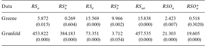
k and RSOHk). The test statistics for both examples are presented in Table 1; thep-values are given in parentheses.
All of the test statistics were computed individually, and the equality in (27) is satis"ed for both data sets. In the example based on Greene's data the
unmodi-"ed tests for serial correlation (RSo) and for random e!ects (RSkto some extent, and RSOk quite strongly) reject the respective null hypothesis of no serial correlation and no random e!ects, and the omnibus test rejects the joint null. But our modi"ed tests suggest that in this example the problem seems to be serial correlation rather the presence of both e!ects. For Grunfeld's data, applications of our modi"ed tests point to the presence of the other e!ect. The unmodi"ed tests soundly reject their corresponding null hypotheses. The
Table 1
Empirical illustration. Tests for random e!ects and serial correlation!
Data RS
k RSHk RSo RSHo RSko RSOk RSOHk
Greene 5.872 0.269 15.569 9.966 15.838 2.423 0.518
(0.015) (0.604) (0.000) (0.002) (0.000) (0.007) (0.3020)
Grunfeld 453.822 384.183 73.351 3.712 457.535 21.303 19.605
(0.000) (0.000) (0.000) (0.054) (0.000) (0.000) (0.000)
!p-values are given in parenthesis.
rather than serial correlation. As expected, the joint test statistic is highly signi"cant.
In spite of the small sample size of the data sets, these examples seem to illustrate clearly the main points of the paper: the proposed modi"ed versions of the test are more informative than a test for serial correlation or random e!ect that ignores the presence of the other e!ect. In the"rst case, serial correlation spuriously induces rejection of the no-random e!ects hypothesis, and in the second case the opposite happens: the presence of a random e!ect induces rejection of the no-serial correlation hypothesis. The joint testRSkorejects the joint null but is not informative about the direction of the misspeci"cation.
RSkoprovides a correct measure of the joint e!ects of individual component and serial correlation. The main problem is how to decompose this measure to get an idea about the true departure(s). From a practical standpoint if
RSko"RSk#RSodoes not hold, that should be an indication of the presence
of an interaction between random e!ects and serial correlation; and the unadjus-ted statistics RS
k and RSo will be contaminated by the presence of other departures. For example, for the Grunfeld data
RS
k#RSo!RSko"RSk!RSHk"RSo!RSHo"69.638.
This provides a measure of the interaction betweenp2kando, and is also equal to the correction needed for each unadjusted test.
5. Monte Carlo results
In this section we present the results of a Monte Carlo study to investigate the
"nite sample behavior of the tests. To facilitate comparison with existing results we follow a structure similar to the one adopted by Baltagi et al. (1992) and Baltagi and Li (1995).
The model was set as a special case of (9):
y
wherea"5 andb"0.5. The independent variablex
itwas generated following
Nerlove (1971):
x
it"0.1t#0.5xi,t~1#uit,
where u
it has the uniform distribution on [!0.5, 0.5]. Initial values were
chosen as in Baltagi et al. (1992). Letp2,p2k,p2
vandp2e represent the variances of u
it, ki,vitandeit, respectively, and letq"p2k/p2, which represents the`strengtha of the random e!ects. Here, p2"p2k#p2
v, and we set p2"20.qand o were
allowed to take seven di!erent values (0, 0.05, 0.1, 0.2, 0.4, 0.6, 0.8), and three di!erent sample sizes (N,¹) were considered: (25, 10), (25, 20) and (50, 10). Since for eachi,v
itfollows an AR(1) process,p2v"p2e/(1!o2). Then, according to this
structure, the random e!ect term and the innovation were generated as
k
i&IIDN(0, 20(1!q)),
e
it&IIDN(0, 20(1!q)(1!o2)).
For each sample size the model described above was generated 1000 times under di!erent parameter settings. Therefore, the maximum standard errors of the estimates of the size and powers would beJ0.5(1!0.5)/1000K0.015. In each replication the parameters of the model were estimated using OLS, and seven test statistics, namely,RSk, RSHk, RSo, RSHo, RSko,RSOk andRSOHkwere computed. The tables and graphs are based on the nominal size of 0.05. Our simulation study was quite extensive; we carried out experiments for all possible parameter combinations for the three sample sizes. We present here only a portion of our extensive tables and graphs; the rest is available from the authors upon request.
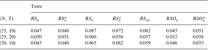
Calculated statistics underq"o"0 were used to estimate the empirical sizes of the tests and to study the closeness of their distributions tos2throughQ}Q plots and the Kolmogorov}Smirnov test. From Table 2 we note that bothRS
k andRSHk have similar empirical sizes, but these are below the nominal size 0.05
forN"25,¹"10 andN"50,¹"10. The results forRS
Table 2
Empirical size of tests. (nominal size"0.05) Tests
(N,¹) RS
k RSHk RSo RSHo RSko RSOk RSOHk
(25, 10) 0.047 0.048 0.087 0.072 0.062 0.045 0.051
(25, 20) 0.050 0.051 0.060 0.056 0.057 0.052 0.058
(50, 10) 0.043 0.040 0.065 0.062 0.059 0.046 0.053
good. All of them reject the null too frequently, but the empirical sizes improve as we increaseNor¹. Comparing the performances ofRS
oandRSHo, we notice thatRSHo has somewhat better size properties. As expected, the one-sided tests RSO
kandRSOHk have larger empirical sizes than their two-sided counterparts. Overall, except for a couple of cases, the size performance of all tests are within one standard errors of the nominal size 0.05.
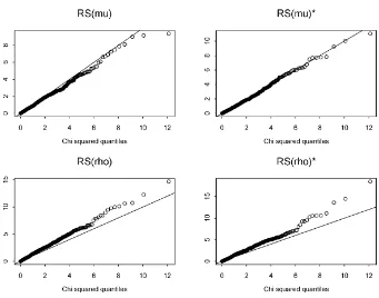
The results of Table 2 are consistent with the Q}Q plots in Fig. 1 for
N"25, ¹"10. To save space"gures for the other two combinations of (N,¹)
are not included. We also do not present the"gures for the joint and one-sided tests, since they resemble those reported for the other tests. From the plots note that the empirical distributions of the test statistics diverge from that of thes21at the right tail parts. For RSk and RSHk the points are below the 453 line, particularly for the high values, and that leads to sizes beingbelow0.05 as we just noted from Table 2. However, the number of points (out of 1000) that are far away from the 453line at the tail parts are not many. For RSo andRSHo we observe a higher degree of departure from the 453line in the opposite direction, and this leads to much higher sizes of the tests. Results from the Kol-mogorov}Smirnov test, not reported here, accept the null hypothesis of the
overalldistribution being the same ass2for the"rst"ve, and standard normal for the last two statistics. For the true sizes of the tests, however, it is only the tail part, not the overall distribution, that matters.
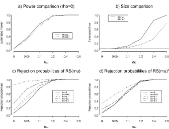
Let us now turn into the performance of tests in terms of power. ForN"25
and ¹"10, the estimated rejection probabilities of the tests are reported in
Table 3, and are also illustrated in Figs. 2(a)}(d). The results forq"o"0.08 are not reported since in most cases the rejection probabilities were one or very close to one. Moreover, our adjusted tests are designed for locally misspeci"ed alternatives close to q"o"0.0, and the main objective of our Monte Carlo study is to investigate the performance of our suggested tests in the neighbor-hood of q"o"0.0. Let us "rst concentrate on RSk,RSHk, RSOk and RSOHk
which are designed to test the null hypothesisH
0: p2k"0. Wheno"0,RSkand
RSO
k are, respectively, the two- and one-sided optimal tests. This is clearly evident looking at all the rows in Table 3 with o"0;RSO
Fig. 1. Q}Qplots. Sample size (25, 10).
powers among all the tests andRSkjust trails behind it. The power ofRSHkis less than that ofRS
kwheno"0. The losses in power are, however, not very large, as can also be seen from Fig. 2(a). Whenqexceeds 0.2 (orp2kexceeds 4, since we set
p2k"20q) both tests have power equal to 1. The amount of loss in usingRSHk
wheno"0 was characterized by (17) in terms of the decrease in the noncentral-ity parameter. That loss increases withq(p2k). However, the overall power ofRSHk
is guided by the noncentrality parameter in (16):
j
6(p2k)"
p4k
2p4e (¹!1)!
p4k
p4e
¹!1
¹ ,
where the second term is the amount of penalty in usingRSHkwheno"0, and it is given in (17). Since the"rst term dominates, the relative value of the loss is negligible. WhileRSHkandRSOHkdo not sustain much loss in power wheno"0, we notice some problems in RSk andRSOk whenp2k"0 but oO0.RSk and RSO
k rejectH0:p2k"0 too frequently. For example, when q"0 (i.e.,p2k"0) ando"0.4,RS
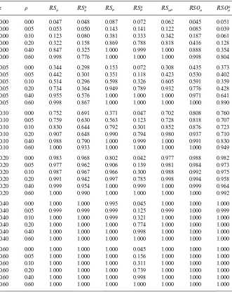
Table 3
Estimated rejection probabilities of di!erent tests. Sample size:N"25;¹"10
q o RS
k RSHk RSo RSHo RSko RSOk RSOHk
0.00 0.00 0.047 0.048 0.087 0.072 0.062 0.045 0.051
0.00 0.05 0.053 0.050 0.143 0.141 0.122 0.085 0.039
0.00 0.10 0.123 0.080 0.381 0.333 0.342 0.187 0.061
0.00 0.20 0.322 0.158 0.869 0.788 0.818 0.416 0.128
0.00 0.40 0.847 0.325 1.000 0.999 1.000 0.888 0.354
0.00 0.60 0.998 0.776 1.000 1.000 1.000 0.998 0.804
0.05 0.00 0.344 0.298 0.153 0.072 0.308 0.435 0.373
0.05 0.05 0.442 0.301 0.351 0.118 0.423 0.530 0.402
0.05 0.10 0.514 0.296 0.598 0.326 0.605 0.591 0.359
0.05 0.20 0.734 0.364 0.949 0.789 0.932 0.776 0.428
0.05 0.40 0.955 0.576 1.000 1.000 1.000 0.971 0.641
0.05 0.60 0.998 0.867 1.000 1.000 1.000 1.000 0.890
0.10 0.00 0.752 0.691 0.371 0.047 0.702 0.808 0.760
0.10 0.05 0.759 0.630 0.563 0.123 0.728 0.818 0.707
0.10 0.10 0.830 0.644 0.792 0.301 0.852 0.876 0.723
0.10 0.20 0.907 0.648 0.990 0.794 0.980 0.937 0.710
0.10 0.40 0.988 0.790 1.000 0.999 1.000 0.991 0.830
0.10 0.60 1.000 0.933 1.000 1.000 1.000 1.000 0.949
0.20 0.00 0.983 0.968 0.802 0.042 0.977 0.988 0.982
0.20 0.05 0.977 0.962 0.906 0.139 0.981 0.984 0.973
0.20 0.10 0.987 0.967 0.966 0.300 0.988 0.992 0.975
0.20 0.20 0.991 0.942 0.997 0.785 0.998 0.994 0.958
0.20 0.40 0.999 0.954 1.000 0.999 1.000 0.999 0.964
0.20 0.60 1.000 0.990 1.000 1.000 1.000 1.000 0.992
0.40 0.00 1.000 1.000 0.995 0.045 1.000 1.000 1.000
0.40 0.05 0.999 0.999 0.999 0.125 0.999 1.000 0.999
0.40 0.10 1.000 1.000 0.999 0.321 1.000 1.000 1.000
0.40 0.20 1.000 1.000 1.000 0.774 1.000 1.000 1.000
0.40 0.40 1.000 1.000 1.000 0.998 1.000 1.000 1.000
0.40 0.60 1.000 1.000 1.000 1.000 1.000 1.000 1.000
0.60 0.00 1.000 1.000 1.000 0.045 1.000 1.000 1.000
0.60 0.05 1.000 1.000 1.000 0.156 1.000 1.000 1.000
0.60 0.10 1.000 1.000 1.000 0.311 1.000 1.000 1.000
0.60 0.20 1.000 1.000 1.000 0.739 1.000 1.000 1.000
0.60 0.40 1.000 1.000 1.000 0.998 1.000 1.000 1.000
0.60 0.60 1.000 1.000 1.000 1.000 1.000 1.000 1.000
true) forRSkcan be seen in Fig. 2(b). As we discussed in Section 3, this unwanted rejection probabilities is due to the noncentrality parameterj
2(o) in (14), which is`purelyaa function of the degree of departure ofofrom zero.RSHk andRSOHk
Fig. 2. Tests for random e!ects. Sample size (25, 10).
For the above case ofq"0 ando"0.4 the rejection probabilities forRSHk and RSOHk are, respectively, 0.325 and 0.354. Fig. 2(b) gives the power ofRSHk when
q"0 for di!erent values of o. As we mentioned earlier, RSHk and RSOHk are designed to be robust only under local misspeci"cation, i.e, for low values ofo. From that point of view, they do a very good job } their performances deteriorate only whenotakes high values. Now by directly comparing the one-and two-sided tests forH
0: p2k"0, we note that the former has higher rejection
probabilities except for a few cases when q"0.0. For these cases the score
L¸/Lp2k takes large negative values and that leads to acceptance ofH
0 when
one-sided tests are used and rejection of H
0 when we use the two-sided test. Note that RSOk"signJRSk rejects H
0 if RSOk'1.645 while using RSk rejection occurs ifRSk'3.84 which exceeds 1.6452.
From Table 3 and Fig. 2(c), we note that whenq'0, an increase ino('0) enhances the rejection probabilities of RSk. For example, when q"0.05 the rejection probabilities of RSk for o"0.0 and 0.2 are, respectively, 0.344 and 0.734. This can be explained using the expression (15), which gives the changes in the noncentrality parameter of RS
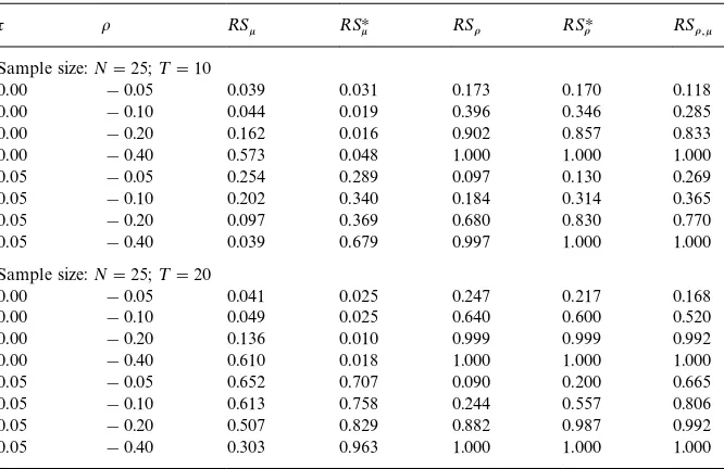
Table 4
Estimated rejection probabilities of di!erent tests for negativeo
q o RS
k RSHk RSo RSHo RSo,k Sample size:N"25;¹"10
0.00 !0.05 0.039 0.031 0.173 0.170 0.118
0.00 !0.10 0.044 0.019 0.396 0.346 0.285
0.00 !0.20 0.162 0.016 0.902 0.857 0.833
0.00 !0.40 0.573 0.048 1.000 1.000 1.000
0.05 !0.05 0.254 0.289 0.097 0.130 0.269
0.05 !0.10 0.202 0.340 0.184 0.314 0.365
0.05 !0.20 0.097 0.369 0.680 0.830 0.770
0.05 !0.40 0.039 0.679 0.997 1.000 1.000
Sample size:N"25;¹"20
0.00 !0.05 0.041 0.025 0.247 0.217 0.168
0.00 !0.10 0.049 0.025 0.640 0.600 0.520
0.00 !0.20 0.136 0.010 0.999 0.999 0.992
0.00 !0.40 0.610 0.018 1.000 1.000 1.000
0.05 !0.05 0.652 0.707 0.090 0.200 0.665
0.05 !0.10 0.613 0.758 0.244 0.557 0.806
0.05 !0.20 0.507 0.829 0.882 0.987 0.992
0.05 !0.40 0.303 0.963 1.000 1.000 1.000
valid only asymptotically and for local departures ofofrom zero. Fig. 2(d) shows that there is some uniform gain in rejection probabilities of RSHk only when
o"0.4. For smaller values of o, the rejection probabilities sometimes even
decrease but are always close to values for the caseo"0. As we indicated earlier there could be somelossof power ofRS
kwheno(0. We performed a small-scale experiment for this case, results of which are reported in Table 4. First note that whenq"0, an increase in the absolute value ofoleads to an increase in the size ofRS
k. For example, whenN"25, ¹"10 andq"0, the rejection frequencies foro"0 and!0.4 are, respectively, 0.047 and 0.573. This is due to the noncentrality parameter (14) which is a function of
o2. Whenq'0 (p2k'0), the changes in the noncentrality parameter could be
negative, and there could be a substantial loss in power ofRSk. For instance, for the above (25, 10) sample size combinations, andq"0.05, the powers of RSk,
for o"0.0 and !0.4 are, respectively, 0.344 and 0.039. RSHk does not su!er
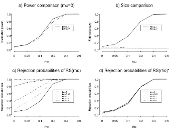
from these detrimental e!ects as we see from Table 4. Its size remains small for allo(0, and power even increases as the absolute value ofobecomes larger. In a similar way, we can explain the behavior ofRSo andRSHo using Table 3 and Figs. 3(a)}(d). From Table 3 we note that, as expected, whenp2k"0,RSo has the highest powers among all the tests. The powers ofRSHo are very close to those of RS
Fig. 3. Tests for serial correlation. Sample size (25, 10).
The real bene"t ofRSHo is noticed wheno"0 butq'0; the performance of RSHois quite remarkable, as can be seen from Fig. 3(b).RS
orejectsH0: o"0 too often, whereas, quite correctly,RSHo does not rejectH
0 so often. For example, whenq"0.2 ando"0, the rejection proportions for RS
o andRSHo are 0.802 and 0.042, respectively. Even when we increaseqto 0.6, the rejection proportion forRSHo is only 0.045, whereasRS
o rejects 100% of the time. In a way,RSHo is doing more than it is designed to do, that is, not rejectingo"0 whenois indeed zero even forlargevalues ofq.
From Fig. 3(c), we observe that the power ofRSois strongly a!ected by the presence of random e!ects, while there is virtually no e!ect on the power ofRSHo
as seen from Fig. 3(d) even for large values of q. This performance ofRSHo is exceptionally good. For negative values ofoin Table 4, we see that the presence of qhas a less detrimental e!ect onRSHo. For example, wheno"!0.10, the rejection probabilities ofRSo are 0.396 and 0.184 forq"0.0 and 0.05, respec-tively; for the same situations, the powers ofRSHo are, respectively, 0.346 and 0.314.
latter in the presence of serial correlation. To see this from a theoretical point of view, let us consider (17) and (22), which are, respectively, the penalties of using RSHkandRSHo. From (17),p4k/p4e(¹!1)/¹, the penalty in usingRSHk, also depends onothroughp2e"20(1!q)(1!o2), while (22), 2o2(¹!1)/¹2, is a function of oonly and is of smaller magnitude in terms of¹.
Finally, we discuss brie#y the performance of the joint statisticRSko in the light of our results (4) and (5). This test is optimal whenp2k'0 andoO0. As we can see from Table 3, in this situationRSkohas the highest power most of the time. However, when the departure fromp2k"0,o"0 is one-directional (say,
p2k'0,o"0),RSkandRSkohave the same non-centrality parameter (see (26)).
SinceRSkoandRSo use thes22 ands21 tests, respectively, there will be a loss of power in usingRSko. For example, whenq"0.10 ando"0, the powers forRSk andRS
ko are 0.752 and 0.702, respectively. Similarly, whenq"0,o"0.2, the power of RS
o and RSko are, respectively, 0.869 and 0.818. These results are consistent with those of Baltagi and Li (1995). AlthoughRS
kohas overall good power, it cannot help to identify the exact source of misspeci"cation when there is only a one-directional departure.
The qualitative performance of all the tests do not change when we increase the sample sizes to N"25, ¹"20, and N"50, ¹"10 and they further illustrate the usefulness of our modi"ed tests. These results are not presented but are available from the authors upon request.
6. Conclusions
In this paper we have proposed some simple tests, based on OLS residuals for random e!ects in the presence of serial correlation, and for serial correlation allowing for the presence of random e!ects. These tests are obtained by adjust-ing the existadjust-ing test procedures. We have investigated the"nite sample size and power performance of these and some of the available tests through a Monte Carlo study. We have also provided some empirical examples. The Monte Carlo study, along with the examples, clearly show the usefulness of our procedures to identify the exact source(s) of misspeci"cation. One drawback of our methodo-logy is that we allow for onlylocalmisspeci"cation. For nonlocal departures, e$cient tests could be obtained after estimating full model(s) by maximum likelihood; that, however, will loose the simplicity of our tests using only OLS residuals.
Acknowledgements
improve the paper. Thanks are also due to Miki Naoko for her help in preparing the manuscript. An earlier version of this paper was presented at Texas A&M University, March 1996; the Midwest Econometric Group Meeting, the University of Wisconsin at Madison, November 1996; the Economics seminar at University of San Andres, Argentina, November 1997; and the Annual Meeting of the Argentine Association of Political Economy, Bahia Blanca, Argentina. We wish to thank the participants and Badi Baltagi for helpful comments and discussion. However, we retain responsibility for any remaining errors.
References
Andereson, T.W., Hsiao, C., 1982. Formulation and estimation of dynamic models using panel data. Journal of Econometrics 18, 47}82.
Balestra, P., Nerlove, M., 1966. Pooling cross-section and time-series data in the estimation of a dynamic model: the demand for natural gas. Econometrica 34, 585}612.
Baltagi, B., 1995. Econometric Analysis of Panel Data. Wiley, New York.
Baltagi, B., Chang, Y., Li, Q., 1992. Monte Carlo results on several new and existing tests for the error component model. Journal of Econometrics 54, 95}120.
Baltagi, B., Li, Q., 1991. A joint test for serial correlation and random individual e!ects. Statistics and Probability Letters 11, 277}280.
Baltagi, B., Li, Q., 1995. Testing AR(1) against MA(1) disturbances in an error component model. Journal of Econometrics 68, 133}151.
Bera, A.K., Jarque, C.M., 1982. Model speci"cation tests: a simultaneous approach. Journal of Econometrics 20, 59}82.
Bera, A.K., Yoon, M.J., 1991. Speci"cation testing with misspeci"ed alternatives. Bureau of Eco-nomic and Business Research Faculty Working Paper 91-0123, University of Illinois, presented at the Econometric Society Winter Meeting, Washington, DC, December 1990.
Bera, A.K., Yoon, M.J., 1993. Speci"cation testing with locally misspeci"ed alternatives. Econo-metric Theory 9, 649}658.
Bera, A.K., Ra, S.S., Sarkar, N., 1998. Hypothesis testing for some nonregular cases in econometrics. In: Chakravorty, S., Coondoo, D., Mukherjee, R. (Eds.), Econometrics: Theory and Practice. Allied Publishers, New Delhi, pp. 319}351.
Breusch, T.S., Pagan, A.R., 1980. The Lagrange multiplier test and its applications to model speci"cation in econometrics. Review of Economic Studies 47, 239}253.
Das Gupta, S., Perlman, M.P., 1974. Power of the noncentral F-test: E!ect of additional variate on Hotteling's¹2-test. Journal of the American Statistical Association 69, 174}180.
Davidson, R., MacKinnon, J.G., 1987. Implicit alternatives and local power of test statistics. Econometrica 55, 1305}1329.
Greene, W., 1983. Simultaneous estimation of factor substitution, economies of scale and non-neutral technical change.. In: Dogramaci, A. (Ed.), Econometric Analyses of Productivity. Kluwer-Nijo!, Boston, pp. 121}144.
Greene, W., 2000. Econometric Analysis, 4th Edition. Prentice-Hall, Englewood Cli!s, NJ. Grunfeld, Y., 1958. The determinants of corporate investment. Unpublished Ph.D. Thesis,
Depart-ment of Economics, University of Chicago.
Grunfeld, Y., Griliches, Z., 1960. Is aggregation necessarily bad? Review of Economics and Statistics 42, 1}13.
Hillier, G.H., 1991. On multiple diagnostic procedures for the linear model. Journal of Econometrics 47, 47}66.
Honda, Y., 1985. Testing the error component model with non-normal disturbances. Review of Economic Studies 52, 681}690.
Hsiao, C., 1986. Analysis of Panel Data. Cambridge University Press, Cambridge.
Lillard, L.A., Willis, R.J., 1978. Dynamic aspects of earning mobility. Econometrica 46, 985}1012. Majunder, A.K., King, M.L., 1999. Estimation and testing of a regression with a serially correlated error component. Working paper, Department of Econometrics and Business Statistics, Monash University, Australia.
Nerlove, M., 1971. Further evidence of the estimation of dynamic economic relations from a time-series of cross-sections. Econometrica 39, 359}382.
Phillips, R.F., 1999. Estimation of mixed-e!ects and error components models with an AR(1) component: some new likelihood maximization procedures and Monte Carlo evidence. Working paper, Department of Economics, George Washington University.
Rao, C.R., 1948. Large sample tests of statistical hypothesis concerning several parameters with applications to problems of estimation. Proceedings of the Cambridge Philosophical Society 44, 50}57.
Saikkonen, P., 1989. Asymptotic relative e$ciency of the classical test statistics under misspeci" ca-tion. Journal of Econometrics 42, 351}369.