www.elsevier.com / locate / econbase
Cointegration analysis using M estimators
*
Ted Juhl
University of Kansas, Department of Economics, 213 Summerfield Hall, Lawrence, KS 66045, USA Received 12 June 2000; accepted 20 December 2000
Abstract
Tests for cointegration are developed using multivariate M estimators. The tests are based on analyzing the singular values of the parameter estimates standardized by the covariance matrix and do not require a reduced rank estimator. 2001 Elsevier Science B.V. All rights reserved.
Keywords: Cointegration; Robust inference
JEL classification: C12; C22
1. Introduction
The dominant strand of the cointegration literature is based on ordinary least-squares (OLS) and reduced rank regression. However, since economic data often exhibit non-Gaussian behavior, it would seem that other estimation strategies may provide an increase in efficiency, translating into increased power in testing. Lucas (1996, 1997, 1998) successfully implemented tests for cointegration using Wald tests, pseudo likelihood ratio tests, and LM tests based on a non-Gaussian likelihood that falls in the class of M estimators.
This paper introduces a new test of cointegrating rank, one which is based on multivariate M estimation of a vector autoregression (VAR). The multivariate M estimator of the first VAR coefficent is standardized by its covariance matrix, and we perform a singular value decomposition. The singular values are tested directly in order to determine the rank of the cointegrating space. This test is called the M singular value test or MSV.
In the remainder of the paper, we use the following standard notation. We denote convergence in
d 1
distribution by →. If W(s) is a Brownian motion with s[(0, 1), then the Lebesgue integrale0W(s) ds
1 ¡ ¡
is denoted byeW and the stochastic integrale0W(s) dW(s) 5eW dW . Finally, if K is a p3r matrix
¡
of full column rank, then K' is a p3( p2r) matrix such that K K' 50.
*Corresponding author. Tel.: 11-785-864-3501; fax:11-785-864-5270. E-mail address: [email protected] (T. Juhl).
2. M-singular value test
We first consider a kth order VAR with iid errors. Let
k21
DXt5m1PXt211
O
GiDXt2i1et, (1) i51where the vectors X andt et are p31, P andGi are p3p, and et has covariance matrix See. Testing the null of r cointegrating vectors involves testing the rank of the matrixP. One way to determine the rank of a matrix is to examine the singular values. The singular values of a matrix K are the
¡
eigenvalues of K K and the rank of a matrix is the number of nonzero singular values. Presumably,
ˆ
we could estimateP, find a standard error forP and calculate the singular values of the standardized
ˆ
P. Finally, we must have some statistical criteria for determining how many of the singular values are significantly different from zero.
We pursue the strategy mentioned above using the class of multivariate M estimators for P. Let
u5(m, P, G, See). We define the estimator ofu as
Suppose that X was a stationary vector and thatt m5Gi50. Then the (stationary) estimator of P,
ˆ
which we denote PM would have an estimated covariance matrix given by
21 21
matrix SC5C1 SccC1 . Next, we construct the standardized matrix
21 / 2 1 / 2
cointegrating vectors can be tested using the statistic MSVr5Toi5r11li. The MSV statistic is
1
asymptotically equivalent to Johansen’s (1988) likelihood ratio statistic if one uses OLS . The asymptotic distribution of MSV is given below.r
¡
Theorem 1. Suppose that assumptions given in Lucas (1998) hold. If rank(P)5r so that P5ab
with a and b both p3r, then
F (s) and F (s) are standard Brownian motions. The correlation between F and F is a diagonal1 2 1 2
1 p ˜
¡ ¡ 21
matrix with the canonical correlations betweena e' t anda'C1 ct. If there is no intercept and one is
¡
¯ ¯
not estimated, F25F . If an intercept is present (and estimated ) and2 a m' 50, F25F22eF . If2
¡ ¯
a'±0, the first element of F is s and the remaining elements are the remaining elements of 2
F22eF .2
The asymptotic distribution of MSV is identical to that of the Wald and LM statistics proposed byr Lucas (1996, 1998). There are nuisance parameters remaining in the limiting distribution in that the Brownian motions are imperfectly correlated, which changes the limiting distribution for each M estimator selected. However, we can find estimates of the correlations and use the Gamma approximation suggested in Boswijk and Doornik (1999) to obtain asymptotic critical values.
3. Monte Carlo
We conduct a simple Monte Carlo experiment using the data generating process
c
] 2 0
DXt5
S D
T Xt211et.0 0
If c50, there are no cointegrating vectors and if c.0, there is one (trivial) cointegrating vector.
2
Several distributions are considered for et; normal, t with 3 degrees of freedom, mixed normal , and
3
Cauchy .
¡
We setr(e)5ln(11e e / 5) so that we use a student-t likelihood with 5 degrees of freedom for the
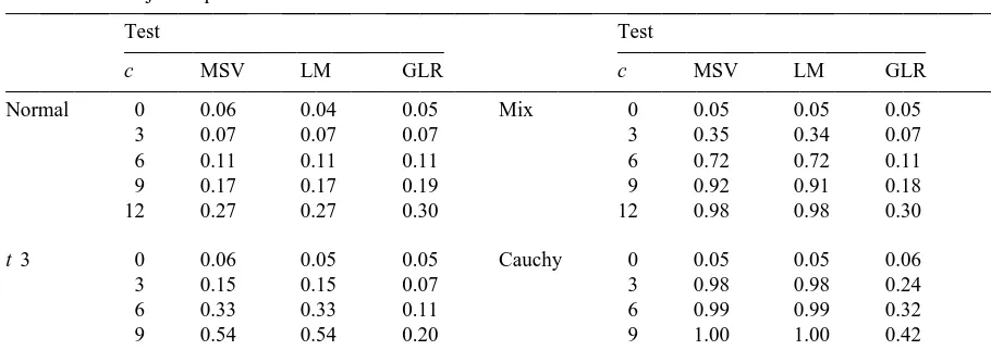
MSV and LM tests. The Gaussian likelihood ratio test of Johansen (1988) is included for comparison and denoted GLR. The sample size is 200 and 10 000 replications are performed. In order to find critical values for the MSV and LM tests, we must find an estimate of the nuisance parameters that affect the limiting distribution. That is, we estimate the canonical correlations between F and F .1 2
Using these estimates, critical values are generated for the tests in each replication by implementing the Gamma approximation proposed in Boswijk and Doornik (1999). The rejection percentage for the tests are listed in Table 1. The MSV test based on the t distribution has good size and power properties and effectively exploits heavy-tailed errors. The Gamma approximation works very well for both the MSV and LM tests.
4. Conclusion
We have developed a new test for cointegrating rank using robust tests based on multivariate M estimators. There are several advantages of the MSV test. First, the test does not depend on the ordering of the variables in the system, a feature shared with the LM test of Lucas (1998). Second, we
2
The observation comes from a normal distribution with standard deviation 2.5 with probability 0.2 and from a normal distribution with standard deviation 0.5 with probability 0.8.
3
Table 1
Size and size adjusted power
Test Test
c MSV LM GLR c MSV LM GLR
Normal 0 0.06 0.04 0.05 Mix 0 0.05 0.05 0.05
3 0.07 0.07 0.07 3 0.35 0.34 0.07
6 0.11 0.11 0.11 6 0.72 0.72 0.11
9 0.17 0.17 0.19 9 0.92 0.91 0.18
12 0.27 0.27 0.30 12 0.98 0.98 0.30
t 3 0 0.06 0.05 0.05 Cauchy 0 0.05 0.05 0.06
3 0.15 0.15 0.07 3 0.98 0.98 0.24
6 0.33 0.33 0.11 6 0.99 0.99 0.32
9 0.54 0.54 0.20 9 1.00 1.00 0.42
12 0.74 0.73 0.31 12 1.00 1.00 0.52
use a Monte Carlo experiment to show that the size and power are quite good. Finally, the computation of the MSV test is particularly simple in that we do not impose a reduced rank condition at the estimation stage, reducing computational complexity compared to the Wald, PLR, and LM tests in Lucas (1996, 1997, 1998). Given the non-linear optimization required for some M estimators, this is highly advantageous.
The proposed MSV test could be easily extended to incorporate adaptively estimated models. Again, we need only obtain one estimate of P adaptively, and consider the singular values from the standardized estimate.
Acknowledgements
´
I thank Bruce Hansen, Roger Koenker, Donald Lien, and Andre Lucas for comments on earlier versions of this paper.
Appendix A. Proof of Theorem 1
We prove the theorem when the data generating process has no intercept and one is not estimated. The other cases are similar. Given the conditions in the theorem,
[Ts ]
ct B (s)c 21 / 2
T
O
S D S D
¡ ⇒b X B (s)
t51 t 2
where B and B are correlated Brownian motions. The variance matrices associated with B and Bc 2 c 2
¡ 21 ¡ ¡ 21 ¡
are Scc and (a b' ') a S a' ee '(b a' ') . Let H5(b,b') be normalized such that H H5I. It is
d
Let the distributions above (not vectorized) be denoted as J1 and J2 respectively. We write
ˆ
are equivalent to the roots of
¡ 21
ˆ ˆ ˆ
ulS112S11PMSC PMS11u
since S11 is positive definite in finite samples. Define
¡ 21
ˆ ˆ ˆ S(l)5lS112S11PMSC PMS .11
¡
Note that S(l) shares the roots of H S(l)H. Using rules for partitioned determinants gives
¡ ¡ ¡ ¡ 21 ¡
uH S(l)Hu5ub S(l)buub'hS(l)2S(l)b(b S(l)b) b S(l)jb'u (A.2) We will consider the asymptotic distribution ofr5Tl since the eigenvalues are normalized by T in
¡
the MSV statistic. Note that under the null hypothesis,r P5ab . Using this fact and the result
¡ ¡ 21 ¡
b'S(l)b'⇒r
E
B B2 2 2D C1 1SccC D1 1 (A.5)¡ ¡ ¡
follows similarly with D15O (1)p a 1(eB B )2 2 J2. Inserting (A.3), (A.4), and (A.5) into (A.2) results in
¡ ¡
ur
E
B B2 2 2D D D2 3 2u (A.6)¡ ¡ 21 21 21 ¡ 21 21
with D25O (1)p a 1eB dB C2 c 1 and D35C1SccC12(C1SccC )1 a(a C1SccC1a) 3
¡ 21
a (C1SccC ). Following Lemma 10.1 in Johansen (1995), we can show that1
¡ 21 21 21 ¡
D35a'(a'C1 SccC1 a') a' ¡
which will eliminate the O (1)p a terms. Then A.6 becomes
¡ 21 ¡ 21 21 21 21 ¡
ur
E
B B2 2 2E
B dB C2 c 1 a'(a'C1 SccC1 a') a'C1E
dB Bc 2u. (A.7)¡ 21 / 2 ¡
Pre and post multiplying A.7 byu(a S a' ee ') (a b' ')uwill not change the roots and it standardizes
B (s) so that all the Brownian motions have unit variance. Then using the trace we have2
p 21
¡ ¡ ¡
˜
T
O
li⇒trS
E
dF F1 2S
E
F F2 2D
E
F dF2 1D
(A.8)i5r11
¡ 21 21 21 / 2 21 ¡ 21 / 2 ¡
where F15(a'C1 SccC1 a') a'C1 B (s) and Fc 25(a S a' ee ') (a b' ')B (s).2 h
References
Boswijk, H., Doornik, J.A., 1999. Distribution approximations for cointegration tests with stationary exogenous regressors. Universiteit van Amsterdam.
Johansen, S., 1988. Statistical analysis of cointegration vectors. Journal of Economic Dynamics and Control 12, 231–254. Johansen, S., 1995. Likelihood-based Inference in Cointegrated Vector Autoregressive Models. Oxford University Press,
New York.
Lucas, A., 1996. Outlier robust unit root analysis. Ph.D. Thesis, Tinberen Institute, Amsterdam.
Lucas, A., 1997. Cointegration testing using pseudolikelihood ratio tests. Econometric Theory 13, 149–169.