www.elsevier.nlrlocaterjappgeo
Hydraulic well testing inversion for modeling fluid flow in
fractured rocks using simulated annealing: a case study at
Raymond field site, California
Shinsuke Nakao
a,), Julie Najita
b,1, Kenzi Karasaki
b,1 aGeological SurÕey of Japan, 1-1-3 Higashi, Tsukuba, Ibaraki, 305-8567, Japan
b
Lawrence Berkeley National Laboratory, Berkeley, CA 94720, USA
Received 2 August 1999; accepted 23 June 2000
Abstract
Ž . Ž .
Cluster variable aperture CVA simulated annealing SA is an inversion technique to construct fluid flow models in fractured rocks based on the transient pressure data from hydraulic tests. A two-dimensional fracture network system is represented as a filled regular lattice of fracture elements. The algorithm iteratively changes element apertures for a cluster of fracture elements in order to improve the match to observed pressure transients. This inversion technique has been applied to hydraulic data collected at the Raymond field site, CA to examine the spatial characteristics of the flow properties in a fractured rock mass. Two major conductive zones have been detected by various geophysical logs, geophysical imaging techniques and hydraulic tests; one occurring near a depth of 30 m and the other near a depth of 60 m. Our inversion results show that the practical range of spatial correlation for transmissivity distribution is estimated to be approximately 5 m in the upper zone and less than 2.5 m in the lower zones. From the televiewer and other fracture imaging logs it was surmised that the lower conductive zone is associated with an anomalous single open fracture as compared to the upper zone, which is an extensive fracture zone. This would explain the difference in the estimated practical range of the spatial correlation for transmissivity.q2000 Elsevier Science B.V. All rights reserved.
Keywords: Hydraulic well test; Inversion; Fluid flow model; Fractured rocks; Simulated annealing
1. Introduction
For engineering concerns such as environmental remediation, it is quite important to characterize
)Corresponding author. Fax:q81-298-61-3702.
Ž .
E-mail addresses: [email protected] S. Nakao ,
Ž .
[email protected] J. Najita , [email protected]
ŽK. Karasaki .. 1
Fax:q1-510-486-5686.
subsurface fractures that control groundwater flow and transport properties of fractured rocks. Pressure interference testing due to pumping or injection us-ing multiple wells is a useful and direct method to collect information on transmissivities of the fracture system. Once pressure transient data is obtained, an inverse method can be applied to match the observed data and hence to construct a hydrological model ŽCarrera and Neuman, 1986; Finsterle, 1993;
. Doughty et al., 1994 .
0926-9851r00r$ - see front matterq2000 Elsevier Science B.V. All rights reserved.
Ž .
Hydrological characterization of fractured rocks is extremely difficult because fracture distributions are highly heterogeneous and discontinuous. If the rock is extensively fractured and all the fractures are hydrologically active, the medium would behave like an equivalent porous medium. However, cross-hole and tracer tests show that this is not usually the case ŽBillaux et al., 1989 . In the case where the rock. matrix can be considered impermeable, major hy-draulic behavior is governed by the geometry of the fracture network. In order to overcome some of these problems, after extracting fracture zones by geologi-cal and geophysigeologi-cal methods, fracture network mod-els with a partially filled lattice were used to
charac-Ž
terize the heterogeneity of the zone Long et al., .
1991 . Our study follows this approach. Ž .
Simulated annealing SA , on the other hand, is a stochastic search method and has attracted attention as a scheme for optimizing the objective function, because the algorithm selects parameters outside the neighborhood of a local minimum. Although in prac-tical applications obtaining the global minimum is not guaranteed, near-optimal solutions can be often found by representing SA as a Markov chain with
Ž
adequate parameters Geman and Geman, 1984; van .
Laarhoven and Aarts, 1987 . SA has been used in a Ž
variety of optimization problems Kirkpatrick et al., .
1983 , and also been applied to geophysical explo-Ž
ration e.g. Sen and Stoffa, 1991; Vasudevan et al., .
1991 , and hydrology to develop a groundwater
man-Ž .
agement strategy Dougherty and Marryott, 1991 Ž
and stochastic reservoir modeling Deutsch and Jour-.
nel, 1994 .
In hydrological applications, Lawrence Berkeley
Ž .
National Laboratory LBNL has been developing an Ž
inverse method for well test data using SA Mauldon .
et al., 1993 . A partially filled lattice represents a fracture network and an individual fracture element is changed randomly from conductive to nonconduc-tive or vice versa. The effect of this change is examined by numerically simulating well tests and comparing simulations with field test data. Jacobsen Ž1993 and Najita and Karasaki 1995 developed a. Ž .
Ž .
SA method called cluster variable aperture CVA SA that uses a distribution of fracture apertures. The algorithm changes element transmissivities by chang-ing element apertures followchang-ing the cubic law. In addition, the algorithm will change the property of a
cluster of elements instead of a single element. Clus-ter size and shape, which represent simplified frac-ture sets, are the parameters specified in the inver-sion. Sensitivity studies, investigating optimal cluster size using synthetic models with spatially correlated transmissivity, showed that the optimal cluster size seems to be 20–40% of the practical range of spatial
Ž
correlation for transmissivity distribution Nakao et .
al., 1999 .
To develop multi-disciplinary field testing tech-niques and analysis methods for characterizing hy-draulic properties of fractured rocks, a dedicated field site was established near the town of Raymond,
Ž .
CA Karasaki et al., 1994 . Questions that are being Ž .
addressed at this site include: 1 the number of boreholes, the number and type of the hydrologic and geophysical well tests needed to characterize a
Ž .
given volume of rock, 2 the possibility of predict-Ž . ing fluid transport based on fracture geometry, 3 how to scale-up the observations made at a smaller
Ž .
scale, and 4 how to relate geometric fracture infor-mation from outcrops and boreholes to hydrology. Various geophysical and hydrologic tests have been conducted in a cluster of nine wells at this site to image the hydrologic connections of a fractured rock mass. The results from these tests indicate that flow is mainly confined in the two dominant upper and
Ž .
lower conductive zones Cohen, 1993 . The prelimi-nary result of hydrologic modeling for the upper conductive zone using SA was presented in Nakao et
Ž .
al. 1999 . In this article, comprehensive results of hydrologic modeling using SA will be presented to examine the spatial characteristics of the flow prop-erties in both the upper and lower conductive zones at the Raymond field site. We will start with a brief description of the Raymond field site, then proceed to describe the hydraulic well testing inversion using SA and the application to the field test data.
2. Raymond field site
mate-Ž
rial in California Bateman and Sawka, 1981; Bate-.
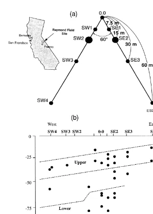
man, 1992 . Nine boreholes were drilled in an in-verted V pattern with increasing spacing between
Ž .
boreholes Fig. 1a . Driller’s logs indicate that rela-tively unweathered granite is located beneath less than 8 m of soil and regolith. The wells are cased to approximately 10 m and vary in depth between 75 and 100 m. The water level is normally between 2 and 3 m below the top of casing.
Various geophysical logs, geophysical imaging techniques and hydraulic tests have been conducted to image the hydrologic connection of the fractured
Ž
rock mass Cohen, 1993; Karasaki et al., 1995; . Cook, 1995; Cohen, 1995; Vasco et al., 1996 . Re-gional characterization and site specific fracture measurements show that there are two sets of subver-tical tectonic fractures: one set strikes at N30W and
Ž .
the other strikes at N60E Cohen, 1995 . The current
Ž . Ž .
Ž .
conceptual model Fig. 1b consists of two dominant conductive zones: one occurring near a depth of 30 m and the other between 54 and 60 m. The presence of these zones are also imaged by ground penetrating radar reflection and a seismic tomography survey ŽVasco et al., 1996 . It should be noted that these. surveys respond to different physical properties, i.e. the seismic method responds to a rock stiffness contrast, while the radar responds to the electro-mag-netic properties of the media. Furthermore, the re-sults from hydraulic tests indicate that there is a high degree of heterogeneity in transmissivity
distribu-Ž .
tions within the two conductive zones Cohen, 1993 . The main purpose of the application of SA is to characterize the heterogeneity of transmissivity dis-tributions within the zones.
3. Analysis method
3.1. SA in general
SA has its origins in thermodynamics and the manner in which liquid metals cool and anneal. In physical annealing, a metal is heated and allowed to cool very slowly in order to obtain a regular molecu-lar configuration having the lowest possible energy state. If the temperature T is held constant, the system approaches thermal equilibrium and the prob-ability distribution for the configuration with energy
Ž .
E approaches the Boltzmann probability Pr E sexp ŽyErk T ; where kb . b is the Boltzmann constant.
Ž .
Metropolis et al. 1953 first introduced a simple algorithm to incorporate these ideas into numerical calculations. The following criterion known as the Metropolis algorithm is applied in determining whether a transition to another configuration occurs at the current temperature. For the ny1st configura-tion Xny1 and the nth configuration Xn with ener-gies Eny1and E , respectively, the transition proba-n bility at some system temperature T is given by
Pr X
Ž
ny1™Xn.
This criterion always allows a transition to a config-uration if system energy is decreased and sometimes allows a transition to a configuration with higher energy. This stochastic relaxation step allows SA to search the space of possible configurations without always converging to the nearest local minimum. In SA, the objective function for an optimization prob-lem is analogous to energy state and the set of free
Ž .
parameters configuration is analogous to the ar-rangement of molecules.ATemperatureB is simply a control parameter in a given optimization problem. We will refer to the objective function as Aobjective
Ž .
function energy B and also refer to the temperature asAcontrol parameter TBin the following sentences. In general, the SA algorithm consists of the
fol-Ž .
lowing tasks: 1 generate or randomly change sys-Ž .
tem configuration, 2 calculate values of the
objec-Ž . Ž .
tive function energy , 3 perform the Metropolis algorithm to determine whether a new configuration
Ž .
is accepted or not, and 4 adjust the current control
Ž .
parameter T according to the annealing cooling schedule.
Several choices of annealing schedule are possi-ble. A computationally practical schedule is the
Ž .
widely used decrement rule Press et al., 1986 . Given an initial control parameter T , assign0
TksT0ak; ks0,1,2,3 . . . ,
Ž .
2where a is between 0 and 1. This general form has
been implemented by others with values of a
rang-Ž
ing from 0.5 to 0.99 e.g. van Laarhoven and Aarts, .
1987 . In this schedule, the current control parameter
T is kept fixed until a finite number of transitions, L , have been accepted, then the parameter T isk
lowered.
3.2. Implementation to well test inÕersion
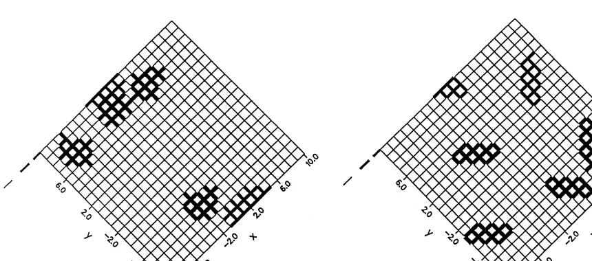
In order to use SA for the inversion of well tests, we consider a two-dimensional fracture network model as shown in Fig. 2. Fractures at multiple depths are not considered. Each element represents a simplified fracture that controls the transmissivity.
Ž 2 . Ž y1.
Transmissivity m rs , specific storage m ,
aper-Ž . Ž .
ture m , unit thickness 1 m and length are imposed on each element. Well locations are specified at node
Ž
Ž .
Fig. 2. Fracture network models: each element represents a simplified fracture. Example of an isotropic fracture cluster left and an
Ž .
anisotropic fracture cluster right .
.
changes due to pumping or injection are calculated at each node using the finite element code TRINET ŽKarasaki, 1987 . Note that the neither SA algorithm. nor TRINET is limited to the two-dimensional model. We use a two-dimensional model because of the complexity and large computational requirements for a 3-D representation. Fluid flow along fractures is assumed to be laminar. It is also assumed that the transmissivity of any fracture element follows the
Ž 3
cubic law Tsrgb r12m — r: density of water, g: acceleration due to gravity, m: dynamic viscosity
.
of water, b: aperture . Whether the cubic law is applicable here is not pertinent to the present study, although the subject itself is very important.
In CVA SA, the objective is to find a near-opti-mal fracture network geometry by modifying clusters
Ž .
of element apertures hence transmissivities and cal-culating pressure transient curves in order to simulta-neously match observed head data at observation wells. At each step of the algorithm, a cluster of elements is randomly selected using the Wolff
algo-Ž .
rithm Wolff, 1989 and their aperture is changed to an aperture chosen at random from a discretized distribution. In this study, we use a finite list of aperture choices. The number and the values of
replacement apertures are user-specified parameters. In the case of Fig. 2, two discretized apertures, thick Žhigh transmissivity and thin low transmissivity. Ž . lines, are specified. The transmissivity of the cluster of elements is also updated according to the cubic law. This step is analogous to the perturbation step in the general SA algorithm.
cluster size increases, however, the cluster shape more likely becomes circular. Instead of the random cluster shape, as shown in Fig. 2, we also have an option in the cluster selection so that the cluster
Ž .
shape can be anisotropic elliptical to incorporate a priori information, namely, geological information about regional fractures such as strikes and scales. These two parameters, cluster size and shape, play a key role in the inversion, because these are a direct representation of simplified fracture sets. As men-tioned before, the optimal cluster size approximately corresponds to the spatial correlation length of
trans-Ž .
missivity distributions Nakao et al., 1999 .
Following the perturbation step, well tests are simulated on the fracture network and the calculated pressure transients are compared with observed data.
Ž .
The objective function energy to be minimized is the sum of the squared differences between the calculated and observed pressure transients due to pumping or injection. In this study, all wells
in-Ž .
cluded in the objective function energy are un-weighted under the assumption that errors in field measurements due to noise or the accuracy of pres-sure transducers are approximately equal for all wells. At the ith iteration:
w x
where ojk refers to the observed pressure transient at the k th time step for jth well. pi jk refers to the simulated pressure transient at the ith iteration for the jth well and k th observed time step.
The Metropolis algorithm is applied to determine whether the current fracture configuration is
accept-Ž .
able based on the Eq. 1 . When L acceptances atk
control parameter T have been achieved, the param-k
Ž .
eter is reduced to Tkq1 via Eq. 2 with as0.9. Tkq1 stays constant until Lkq1transitions have been accepted at Tkq1. This process continues until the annealing schedule is exhausted or the number of iterations has reached a user-specified maximum. At this point, the best model found thus far is expected to be close to the global minimum. In the following,
Ž .
we refer to Aminimum objective function energyB; however, this is used to describe the smallest
objec-Ž .
tive function energy found at the end of the inver-sion.
4. Hydraulic well test data
Hydraulic well testing was conducted at the Ray-Ž
mond field site on several occasions e.g. Cohen, 1993; Karasaki et al., 1995; Cook, 1995; Cohen,
.
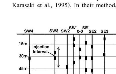
1995 . The data used in this study was taken in 1995. Each of the nine wells was injected systematically with fresh water using a straddle packer system. The distance between the straddle packers was roughly 6 m. A typical injection test was conducted for 10 min. The pressure in the water tank was held constant using compressed air. Neither the flow rate nor the downhole pressure was actively controlled; they spontaneously adjusted themselves accordingly to the transmissivity of the injection interval. The ad-vantages of this method are the simplicity of the set-up and the ease of test execution. After each test, the packer string was lowered by approximately 6 m. Depth intervals sealed by packers during a particular injection were kept unobstructed during the next, so that the entire length of the well was tested. There were approximately 15 injection tests per well in all nine wells. While these injections were conducted, the pressures in the remaining 31 intervals were simultaneously monitored. As a result, a total of 4200 interference pressure transients were recorded. A schematic of the packer set up in the site is shown in Fig. 3. To analyze connections between wells using a large number of interference data, a binary
Ž
inversion method was developed Cook, 1995; .
Karasaki et al., 1995 . In their method, each set of
pressure transient data was reduced to a binary set: 1 Žyes if an observation zone responds to an injection,.
Ž .
and 0 no otherwise, and they successfully visual-ized connections between wells. The result strongly supports the existence of two separated conductive zones, one at a depth of approximately 30 m and other at 60 m.
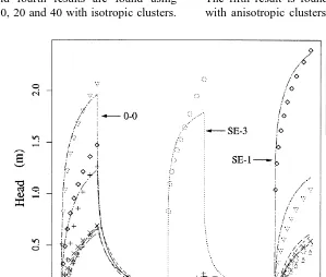
From the large number of interference data de-scribed above, three sets of injection data in series were selected for each zone: injection into wells 0-0, SE-1 and SE-3 for the upper zone, and injection into wells 0-0, SW-1 and SW-3 for the lower zone. These injection intervals are located approximately between depths of 20 to 30 m and between depths of 50 to 60 m. Intervals with interference response are also lo-cated in these depths. We believe these intervals are confined in the upper and lower conductive zones shown in Fig. 1b. Injection flow rates were, on the average, 6.4 lrmin for well 0-0, 5.9 lrmin for well SE-1 and 6.5 lrmin for well SE-3 in the upper zone. In the lower zone, injection flow rates were 4.5 lrmin for well 0-0, 5.3 lrmin for well SW-1 and 1.4 lrmin for well SW-3. It should be noted that for a pair of wells, injecting at the first and observing at the second does not always give the same pressure
Ž
response when their roles are reversed i.e. injecting .
at the second and observing at the first . For exam-ple, injection into well 0-0 gives about 1.5 m change of head in well SE-3; on the other hand, injection into well SE-3 gives 0.2 m change of head in well
Ž .
0-0 for the upper zone see Fig. 6 . This is because the packer configurations were changed before doing the reciprocal tests.
Ž .
The template model of the site consists of a 32=32 regular grid with 2.5 m fracture elements which covers an 80=80 m area both for the upper and lower zones. The total number of nodes and elements are 1089 and 2112, respectively. Wells SW-4 and SE-4 are not included in the model, because the interference response is not observed during a 600-s injection. In all the calculations dis-cussed below, we impose an initial head value of 0 m for all nodes, so that the relative head changes of wells are examined. We also assign constant pressure
Ž .
conditions 0 m on the outer boundary. As an initial configuration, all fracture elements have
transmissiv-y5 Ž 2 . y4
ity 10 mrs , aperture 2.30=10 m. This ini-tial transmissivity is the average value of the aquifer
estimated from the drawdown analyses of the three
Ž .
wells, 0-0, SW-1 and SE-1 Cohen, 1993 . Note that the transmissivity of the outer region beyond a radius of 37.5 m from the origin is held fixed at 10y5 Ž 2 .
m rs throughout the inversion, because the pres-sure transients are not so sensitive to the transmissiv-ity distribution of the outer region. In other words, it is difficult to resolve the regions away from the wells and in particular, the regions near the bound-aries.
The equivalent specific storage of the fracture elements are set to be 0.1 and 0.01 my1 for the upper and lower zones, respectively, and are held constant throughout the inversion. These values are selected by trial and error. It is generally necessary to use a higher-than-usual specific storage in discrete fracture network models where the conductivity of an element is coupled to its volume through the cubic law. Because it is impossible to model all the fractures and pore spaces in the rock enumeratively due to the computational limitations, the specific storage value in the model is an effective one that represents the storage of the volume of rock that
Ž .
surrounds the fracture element. Mauldon et al. 1993 used a similar approach for their simulation of the fracture flow experiments conducted at Stripa Mine in Sweden. Our focus, too, is to estimate the distribu-tion of the transmissivity contrast. Therefore, we feel it is justified to use the effective value for the specific storage.
In our forward simulation, we set the boundary condition at the well as the constant rate using the average flow rate over the injection period. Except for the very early time, when the compliance of the injection plumbing affected the apparent flow rate, the flow did not change greatly. Replacement aper-tures specified in the inversion are 1.07=10y3, 4.96=10y4, 2.30=10y4and 1.07=10y4 m, which correspond to transmissivities of 10y3, 10y4, 10y5
y6 Ž 2 .
and 10 mrs , respectively. The upper and lower zones were modeled separately.
5. Results
5.1. The upper zone
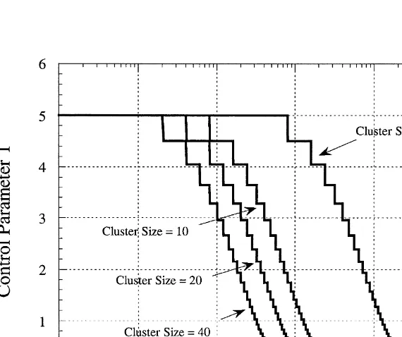
the transmissivity distribution within the upper con-ductive zone. For each cluster size, inversions were run seven times starting from seven different random seeds. Inversions using cluster size of 10 with anisotropic clusters, with strikes at N30W and N60E, were also conducted. These major fracture sets were identified from the measurements of outcrops and
Ž .
the acoustic televiewer logs. Annealing cooling schedules for four cluster sizes are shown in Fig. 4. In these schedules, the total number of the element change in an inversion is set to be same for all cluster size cases. Namely, in the case of cluster size 40, the control parameter T is lowered after 20 configuration changes are accepted, whereas the con-trol parameter T is lowered after 800 changes are accepted in the case of cluster size 1. We set all inversions will be stopped when the annealing sched-ule is exhausted. This means that the inversions using larger cluster sizes need less number of itera-tion. For example, the inversions using cluster sizes 1 and 40 requires approximately 22,460 and 980 total iterations, respectively.
Fig. 5 summarizes the inversion results. The
low-Ž .
est minimum objective function energy , 4.7, is
reached in the seed 4 of the cluster size 10, starting
Ž .
from the initial objective function energy of 3.33=
3 Ž .
10 . The minimum objective function energy varies to some extent depending on a random seed for a given cluster size. The averaged minimum objective
Ž .
function energy is smallest for a cluster size of 1. As the cluster size decreases, the averaged minimum
Ž .
objective function energy also decreases. Compari-son of pressure transients between observed and calculated data for the minimizing configuration
ob-Ž .
tained using the cluster size 10 seed 4 is illustrated in Fig. 6. A relatively good match is achieved.
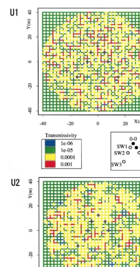
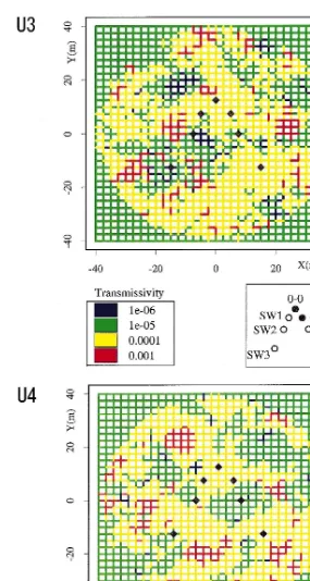
In order to represent average properties of the annealing solutions obtained using the same cluster size, seven annealing solutions are combined to pro-duce one configuration by means of median filters, which are commonly used as velocity filters in data
Ž
processing of vertical seismic profiling e.g. Hardage, .
1985 . That is, the median transmissivity value Žtransmissivity value itself, not its logarithm among. seven values is selected for each fracture element so as to produce one median configuration. Five me-dian-filtered configurations are shown in Figs. 7–9. The first result is found using a cluster size of 1. The
Ž .
Ž .
Fig. 5. Inversion results for the upper zone: minimum objective function energy vs. cluster sizes.
second, third and fourth results are found using cluster sizes of 10, 20 and 40 with isotropic clusters.
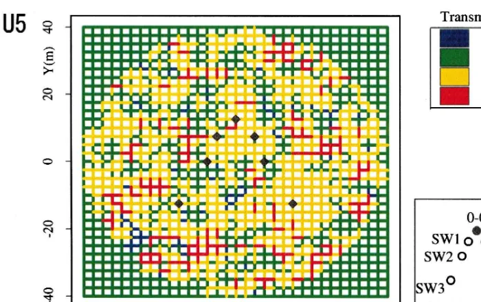
The fifth result is found using a cluster size of 10 with anisotropic clusters, with strikes at N30W and
Ž .
Ž . Ž .
Fig. 7. Median-filtered inversion result with cluster size 1 U1 and cluster size 10 U2 for the upper zone. The injection test data into well
Ž .
Ž . Ž .
Ž .
Fig. 9. Median-filtered inversion result with cluster size 10 and anisotropic shapes for the upper zone U5 .
N60E. We refer to these as cases U1 through U5. It is difficult to observe the major feature common to all the results from these figures. However, the an-nealing results consistently show high transmissivi-ties around well 0-0. SW-3 is relatively isolated in U3 and U5 results. This is because SW-3 had a very low interference response from all of three well
Ž .
injections see Fig. 6 . Aside from these two
fea-Ž .
tures, U1–U4 isotropic clusters do not seem to show a particular spatial pattern.
Since the inversion result is based on limited information and the hydraulic inversion is inherently non-unique, it is difficult to say how ArealB such results are. Rather, we believe that assessing the validity of the result can best be done by testing how
Ž .
the result model predicts hydraulic behavior of the data, which is not used to build the model. Thus, to evaluate the inversion results, a cross validation test was conducted. We modeled the SW-2 injection test, which was not included in the inversion as injection
Ž .
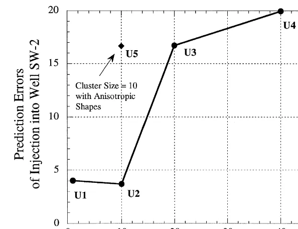
data. TRINET Karasaki, 1987 was again used to simulate injection into SW-2. Fig. 10 shows predic-tion errors for injecting at SW-2 for each cluster size
Ž .
results U1–U5 . The prediction error, which is the sum of the squared difference between the calculated
Ž .
and observed data given by Eq. 3 , is approximately 4 for cases U1 and U2, while it is more than 15 for
U3, U4 and U5. This result indicates that cases U1 and U2 are the good models among the results of five cluster types. From these results, we observe that cluster sizes of 1 and 10 are suitable to obtain good results.
Ž The omnidirectional semi-variogram for U2
clus-.
ter size of 10 is given in Fig. 11. The directional semi-variograms were also calculated to check the existence of geometric anisotropies. However, no significant anisotropies are observed in Fig. 11. A practical range of the spatial correlation is
approxi-Ž
mately 4.0 m since both the element length and . spacing are 2.5 m, we refer to this value as 5.0 m . This practical range is a little smaller than that obtained from each annealing solution because of the smoothing effect of the median filters. However, it is
Ž .
nearly consistent with the range 5–7.5 m estimated from the optimal cluster size, in that the optimal cluster size corresponds to 20–40% of the number of fractures within the practical range of spatial
correla-Ž .
tion Nakao et al., 1999 .
5.2. The lower zone
re-Fig. 10. Predicted errors of injection into well SW-2 for five annealing solutions for the upper zone.
Ž sults. The lowest minimum objective function
en-.
ergy , 140.0, is reached in the seed 7 of the cluster size 1, starting from the initial objective function Ženergy of 4.82. 3
=10 . The averaged minimum
ob-Ž .
jective function energy is smallest for a cluster size
of 1. As the cluster size decreases, the minimum
Ž .
objective function energy also decreases. For clus-ter size of 10, the anisotropic-shapes case reaches smaller energy than that of isotropic-shapes case. Comparison of pressure transients between observed
Ž .
Ž .
Fig. 12. Inversion results for the lower zone: minimum objective function energy vs. cluster sizes.
and calculated data for the minimizing configuration
Ž .
obtained using the cluster size 1 seed 7 is
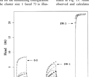
illus-trated in Fig. 13. Although a good match between observed and calculated data was obtained in the
Ž .
Ž . Ž .
Fig. 14. Median-filtered inversion result with cluster size 1 L1 and cluster size 10 L2 for the lower zone. The injection test data into well
Ž .
Ž . Ž .
Ž .
Fig. 16. Median-filtered inversion result with cluster size 10 and anisotropic shapes for the lower zone L5 .
lower zone, the absolute head value of the injection into SW-3 is quite large. This causes the relatively
Ž .
high minimum objective functions energies rather than those of the upper zone cases.
Five median-filtered configurations are shown in Figs. 14–16. The first result is found using a cluster size of 1. The second, third and fourth inversion solutions are found using cluster sizes of 10, 20 and
Ž .
Fig. 18. Omnidirectional and directional semi-variograms of transmissivity for the inversion results with cluster sizes1 L1 for the lower zone.
40 with isotropic clusters. The fifth result is found using a cluster size of 10 with anisotropic clusters, with strikes at N30W and N60E. We refer to these as cases L1 through L5. A major feature common to all the results is that well SW-3 is clearly isolated. This is because SW-3 had a very high head change while
Ž .
injection see Fig. 13 . Annealing results also show a relatively high transmissivity area between wells SW-2 and SE-2.
In order to evaluate the inversion results, a cross validation test was again conducted. We modeled the SW-2 and the SE-1 injection tests, which were not included in the inversion as injection data. Fig. 17 shows predicted errors for injecting at SW-2 and
Ž .
SE-1 for each cluster size results L1–L5 . For clus-Ž . ter size of 10, the anisotropic-shapes case L5 ob-tains smaller error than that of isotropic-shapes case ŽL2 . This finding will be discussed in the next. section. The prediction errors are smallest for L1 in
Ž both injections. This result indicates that L1 cluster
.
size of 1 is the most suitable among the results of five cluster types.
The directional and omnidirectional
semi-vario-Ž .
grams for L1 cluster size of 1 are given in Fig. 18. A practical range of the spatial correlation is less
Ž
than 2.5 m since both of the element length and . spacing are 2.5 m, we refer to this value as 2.5 m . This practical range is consistent with the range Žaround 2.5 m estimated from the optimal cluster.
Ž .
size Nakao et al., 1999 . It is impossible to observe whether geometric anisotropies of the correlation structure exist within the range of 2.5 m, because of the resolvable scale used in the configuration. Note that this is the first attempt to estimate the horizontal correlation length of transmissivity for both the up-per and lower conductive zones at Raymond field site.
6. Discussion
In the preliminary analysis of the upper zone ŽNakao et al., 1999 , we conducted the SA inversion. just once for each cluster size, resulting in a little overestimation of the practical range of the spatial
Ž .
correlation for transmissivity 5–10 m . In this study,
Ž .
stacked to produce one average configuration by means of the median filters. This is because we really want to extract the average properties of the transmissivity distribution, which may be specific for the results obtained using each cluster size.
For the upper zone, we showed that the configura-tion achieved using cluster size of 1 or 10 with
Ž .
isotropic cluster shapes cases U1 or U2 are the most suitable among five cluster types for obtaining good fluid flow models. Furthermore, the inversion using cluster size of 10 requires approximately one tenth of the iteration number for the cluster size of 1, which means that the cluster size of 10 is optimal to enhance convergence of the inversion from the view-point of computational effectiveness. From the semi-variogram analysis of U2, the practical range of the correlation structure is estimated to be 5.0 m, and no obvious geometric anisotropies are observed.
For the lower zone, we showed that the
configura-Ž .
tion achieved using cluster size of 1 case L1 is the most suitable among five cluster types for obtaining good fluid flow models. On the other hand, both of
Ž .
the minimum objective function energy and predic-tion errors are smaller for the anisotropic cluster
Ž .
shape case L5 than those for the isotropic cluster Ž .
shapes case L2 . This suggests the possibility of the lower zone being anisotropic with possible strikes at N30W and N60E, and that the geometric fracture information from outcrops and boreholes may be correlated to hydrology. Even though this is the case, the practical range of the correlation structure is estimated to be less than 2.5 m from the
semi-vario-Ž . gram analysis of the best result L1 .
From the televiewer, television and optical scan-ner logs it was determined that the lower zone is associated with an anomalous single open fracture as compared to the upper zone, which is an extensive fracture zone. This would explain the difference in the estimated practical range of the spatial
correla-Ž .
tion for transmissivity. Vasco et al. 1996 analyzed
Ž .
seismic velocity structures and Q attenuation struc-tures at this site and reported that the velocity and attenuation anomalies appeared to coincide with the extensively fractured upper zone, although some dis-crepancies between the velocity and attenuation anomalies existed in the lower zone. They suggest that velocity and attenuation anomalies indicate frac-ture zones rather than individual fracfrac-tures. This also
supports the difference in fracture types between the upper and lower conductive zones.
We showed that the process of selecting a reason-able cluster size and shape using this algorithm by trial and error may lead to an estimated range of spatial correlation. With a possible range of spatial correlation parameters, we have much more valuable information, such as how to extrapolate model re-sults to a larger region. Note that a cluster size of, say, five can be used to fine-tune the optimal cluster size. However, because we chose to use an orthogo-nal lattice, the resolvable length scale is nonetheless limited to the multiple of 2.5 m when we estimate the practical range of spatial correlation for transmis-sivity.
It is important to conduct cross validation tests to determine the variability in solutions, because the models we build use very limited data. This differs from building models based on a complete knowl-edge of the ArealB fracture system. For future study, in order to reduce the uncertainty in the hydrological model, inversion of both hydraulic and tracer test data is planned, because the tracer test data analysis is more effective to estimate fluid flow paths within the fracture network. It is also important to conduct sensitivity studies to develop a field test design, such as the relative number of injection or pumping wells and observation wells, and the location of the wells. These factors are clearly related to the ability to detect heterogeneity of the hydraulic conductivity structure.
7. Conclusions
seven annealing solutions are combined to produce one configuration by means of median filters.
Since a cluster size of 1 and 10 gives the
mini-Ž .
mum objective function energy , the practical range of the spatial correlation of transmissivity is esti-mated to be 5 m in the upper extensive fracture zone. On the other hand, the practical range of the spatial correlation of transmissivity is estimated to be less than 2.5 m in the lower fracture zone, because the cluster size of 1 gives minimum objective function Ženergy . These results are confirmed by the cross. validation of the injection test data, which is not used in the inversion.
Acknowledgements
This work was supported by Science and
Tech-Ž .
nology Agency of Japan STA . It was also partially supported by the Japan Nuclear Cycle Development
Ž .
Institute JNC , through the U.S. Department of En-ergy Contract Number DE-AC03-76SF00098. We would like to thank two anonymous reviewers for their helpful comments.
References
Bateman, P.C., 1992. Plutonism in the central part of the Sierra
Ž .
Nevada Batholith, Professional Paper No. 1483 . U.S. Geo-logical Survey, 186.
Bateman, P.C., Sawka, W.N., 1981. Raymond Quadrangle, Madera and Mariposa Counties, California — Analytic data. USGS Professional Paper No.1214.
Billaux, D., Chiles, J.P., Hestir, K., Long, J., 1989. Three-dimen-sional statistical modelling of a fractured rock mass — an example for the Fanay–Augers mine. Int. J. Rock Mechanics
Ž .
Mining Sci. 26 3r4 , 281–299.
Carrera, J., Neuman, S.P., 1986. Estimation of aquifer parameters under transient and steady state condition: 2. Uniqueness, stability, and solution algorithm. Water Resour. Res. 22, 211– 227.
Cohen, A.J.B., 1993. Hydrogeologic characterization of a frac-tured granite rock aquifer, Raymond, CA. MSc Thesis, Univ. of California, Lawrence Berkeley Laboratory, LBL-34838, Berkeley, 97.
Cohen, A.J.B., 1995. Hydrogeologic characterization of fractured rock formation: a guide for groundwater remediators. Lawrence Berkeley National Laboratory report, LBL-38142, Berkeley, 144.
Cook, P., 1995. Analysis of hydraulic connectivity in fractured
granite, MSc Thesis, Univ. of California. Lawrence Berkeley National Laboratory report, Berkeley, 70.
Deutsch, C.V., Journel, A.G., 1994. Integrating well test-derived effective absolute permeability in geostatistical reservoir
mod-Ž .
eling. In: Yarus, J.M., Chambers, R.L. Eds. , Stochastic Modeling and Geostatistics. AAPG, pp. 131–141.
Dougherty, D., Marryott, R.A., 1991. Optimal groundwater man-agement: 1. Simulated annealing. Water Resour. Res. 27, 2493–2508.
Doughty, C., Long, J.C., Hestir, K., Benson, S.M., 1994. Hydro-logic characterization of heterogeneous geoHydro-logic media with an inverse method based on iterated function systems. Water Resour. Res. 30, 1721–1745.
Finsterle, S., 1993. ITOUGH2 user’s guide version 2.2. Lawrence Berkeley National Laboratory report, LBL-34581, Berkeley, 102.
Geman, S., Geman, D., 1984. Stochastic relaxation, Gibbs distri-bution and Bayesian restoration of images. IEEE Trans. Pat-tern Analysis Machine Intelligence, PAMI 6, 721–741. Hardage, B.A., 1985. Vertical seismic profiling: Part A:
Princi-ples, Handbook of Geophysical Exploration. Geohysical Press. Jacobsen, J.S., 1993. A user’s and programmer’s guide to anneal: A research code developed to implement simulated annealing for hydraulic well test applications. Technical report, Lawrence Berkeley Laboratory, Berkeley, 58.
Karasaki K., 1987, A new advection–dispersion code for calculat-ing transport in fracture networks. Earth Sciences Division Annual Report 1986. LBL-22090, Berkeley, pp. 55–58. Karasaki, K., Freifeld, B., Davison, C., 1994. A characterization
study of fractured rock. Proceedings of Internat. High Level Radio. Waste Manag. Conf. pp. 2423–2428.
Karasaki, K., Cohen, A., Cook, P., Freifeld, B., Grossenbacher, K., Peterson, J., Vasco, D., 1995. Hydrologic imaging of fractured rock. Proceedings of Materials Research Society Symposium vol. 353, pp. 379–386.
Kirkpatrick, S., Gelatt, C.D. Jr., Vecchi, M.P., 1983. Optimization by simulated annealing. Science 220, 671–680.
Long, J.C.S., Karasaki, K., Davey, A., Peterson, J., Landsfeld, M., Kemeny, J., Martel, S., 1991. An inverse approach to the construction of fracture hydrology models conditioned by geophysical data. Int. J. Rock Mech. Mining Sci. Geomech.
Ž .
Abstr. 28 2r3 , 121–142.
Metropolis, N., Rosenbluth, A., Rosenbluth, M., Teller, A., Teller, E., 1953. Equation of state calculations by fast computing machines. J. Chem. Phys. 21, 1087–1092.
Mauldon, A.D., Karasaki, K., Martel, S.J., Long, J.C.S., Lands-feld, M., Mensch, A., Vomvoris, S., 1993. An inversion technique for developing models for fluid flow in fracture systems using simulated annealing. Water Resour. Res. 29, 3775–3789.
Nakao, S., Najita, J., Karasaki, K., 1999. Sensitivity study on hydraulic well testing inversion using simulated annealing. Ground Water 37, 736–747.
Press, W.H., Flannery, B.P., Teukolsky, S.A., Vetterling, W.T., 1986. Numerical Recipes: The Art of Scientific Computing. Cambridge Univ. Press, 818.
Sen, M.K., Stoffa, P.L., 1991. Nonlinear one-dimensional seismic waveform inversion using simulated annealing. Geophysics 56, 1624–1638.
van Laarhoven, P.J.M., Aarts, E.H.L., 1987. Simulated Annealing: Theory and Applications. D. Reidel Publishing, 186.
Vasco, D.W., Peterson, J.E. Jr., Majer, E.L., 1996. A simultane-ous inversion of seismic traveltimes and amplitudes for veloc-ity and attenuation. Geophysics 61, 1738–1757.
Vasudevan, K., Wilson, W.G., Laidlaw, W.G., 1991. Simulated annealing statics computation using an order-based energy function. Geophysics 56, 1831–1839.
Wolff, U., 1989. Collective Monte Carlo updating for spin
sys-Ž .