Comparation on Several Smoothing Methods in
Nonparametric Regression
R. Rizal Isnanto
Abstract – There are three nonparametric regression methods covered in this section. These are Moving Average Filtering-Based Smoothing, Local Regression Smoothing, and Kernel Smoothing Methods. The Moving Average Filtering-Based Smoothing methods discussed here are Moving Average Filtering and Savitzky-Golay Filtering. While, the Local Regression Smoothing techniques involved here are Lowess and Loess. In this type of smoothing, Robust Smoothing and Upper-and-Lower Smoothing are also explained deeply, related to Lowess and Loess. Finally, the Kernel Smoothing Method involves three methods discussed. These are Nadaraya-Watson Estimator, Priestley-Chao Estimator, and Local Linear Kernel Estimator. The advantages of all above methods are discussed as well as the disadvantages of the methods.
Keywords: nonparametric regression, smoothing, moving average, estimator, curve construction.
I. INTRODUCTION
Nowadays, maybe the names “lowess” and “loess” which are derived from the term “locally weighted scatterplot smoothing,” as both methods use locally weighted linear regression to smooth data, is often discussed. Finally, the methods are differentiated by the model used in the regression: lowess uses a linear polynomial, while loess uses a quadratic polynomial [3]. A very popular technique for curve fitting complicated data sets is called lowess ([1], [2]) (locally weighted smoothing scatter plots, sometimes called
loess). In lowess, the data is modeled locally by a
polynomial weighted least squares regression, the weights giving more importance to the local data points. This method of approximating data sets is called locally
weighted polynomial regression. The power is lowess is
that you do not require a fit function to fit the data (a smoothing parameter and degree of the local parameter (usually 1 or 2) is supplied instead). The disadvantage in using lowess is that you do not end up with an analytic fit function (yes, this was an advantage as well). Also, lowess works best on large, densely sampled data sets.
However, in this paper, we will also discuss other smoothing methods, started with Moving Average-Based Smoothing, Local Regression Smoothing, where Lowess and Loess are involved here, and finally, Kernel
Smoothing Method, completed with its variants will be also analyzed. The advantages of all above methods are discussed as well as the disadvantages of the methods.
Moving average filtering is the former of smoothing techniques. A moving average filter smooths data by
where ys(i) is the smoothed value for the ith data point,
N is the number of neighboring data points on either
side of ys(i), and 2N+1 is the span.
The moving average smoothing method used commonly follows these rules: the span must be odd; the data point to be smoothed must be at the center of the span; the span is adjusted for data points that cannot accommodate the specified number of neighbors on either side; and that the end points are not smoothed because a span cannot be defined.
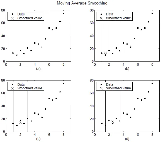
The smoothed values and spans for the first four data points of a generated data set are shown in Fig. 1.
The newer method based on moving average filtering is Savitzky-Golay filtering. This method can be thought of as a generalized moving average. You derive the filter coefficients by performing an unweighted linear least squares fit using a polynomial of a given degree. For this reason, a Savitzky-Golay filter is also called a digital smoothing polynomial filter or a least squares smoothing filter. Note that a higher degree polynomial makes it possible to achieve a high level of smoothing without attenuation of data features.
The Savitzky-Golay filtering method is often used with frequency data or with spectroscopic (peak) data.
Figure 1. Plot (a) indicates that the first data point is not smoothed because a span cannot be constructed. Plot (b) indicates that the second data point is smoothed using a span of three. Plots (c) and (d) indicate that a span of five is used to calculate the smoothed value.
For frequency data, the method is effective at preserving the high-frequency components of the signal. For spectroscopic data, the method is effective at preserving higher moments of the peak such as the line width. By comparison, the moving average filter tends to filter out a significant portion of the signal’s high-frequency content, and it can only preserve the lower moments of a peak such as the centroid. However, Savitzky-Golay filtering can be less successful than a moving average filter at rejecting noise.
The newer method based on moving average filtering is Savitzky-Golay filtering. This method can be thought of as a generalized moving average. You derive the filter coefficients by performing an unweighted linear least squares fit using a polynomial of a given degree. For this reason, a Savitzky-Golay filter is also called a digital smoothing polynomial filter or a least squares smoothing filter. Note that a higher degree polynomial makes it possible to achieve a high level of smoothing without attenuation of data features.
The Savitzky-Golay filtering method is often used with frequency data or with spectroscopic (peak) data. For frequency data, the method is effective at preserving the high-frequency components of the signal. For spectroscopic data, the method is effective at preserving higher moments of the peak such as the line width. By comparison, the moving average filter tends to filter out a significant portion of the signal’s high-frequency content, and it can only preserve the lower moments of a peak such as the centroid. However, Savitzky-Golay filtering can be less successful than a moving average filter at rejecting noise.
The Savitzky-Golay smoothing method used commonly follows these rules: the span must be odd; the polynomial degree must be less than the span; and the data points are not required to have uniform spacing.
Normally, Savitzky-Golay filtering requires uniform spacing of the predictor data. However, the algorithm provided supports nonuniform spacing. Therefore, you are not required to perform an additional filtering step to create data with uniform spacing.
3
Figure 3. The graph on the left is a seemingly good fit (α = 0:2); the graph in the middle has been over smoothed (α = 0:4); the graph on the right is
under smoothed (α = 0:05).
The plot shown in Fig. 2 displays generated Gaussian data and several attempts at smoothing using the Savitzky-Golay method. The data is very noisy and the peak widths vary from broad to narrow. The span is equal to 5% of the number of data points.
From Fig. 2, it can be shown that plot (a) shows the noisy data. To more easily compare the smoothed results, plots (b) and (c) show the data without the added noise. Plot (b) shows the result of smoothing with a quadratic polynomial. Notice that the method performs poorly for the narrow peaks. Plot (c) shows the result of smoothing with a quartic polynomial. In general, higher degree polynomials can more accurately capture the heights and widths of narrow peaks, but can do poorly at smoothing wider peaks.
III.LOCAL REGRESSION SMOOTHING PROCEDURE
The curve obtained from a loess model is governed by two parameters, α and λ. The parameter α is a smoothing functions are used to approximate globally complicated data sets. To use cubic polynomials or other more complex functions for the local approximation, although allowed in the theory, would go against the “simple local function” idea underlying lowess. Fig. 3 shows some parameter α. We can see that over or under-smoothing the data can make your lowess fit not as good as you may like. Oversmoothing reveals general trends, but obscures the local variations. Under smoothing results in a
“choppy” fit, for which there is too much local variation. Neither of these situations is desirable.
So the question becomes, how can we choose the best value for α? Since there is interplay between the local polynomial that is chosen and the smoothing parameter, the first thing we should say is that typically the local polynomial is kept as simple as possible, and the smoothing parameter is then varied. So begin your analysis with a linear local polynomial, and then vary the smoothing parameter until your curve approximates the data well. Typically, smoothing parameters in the range 0.2–0.5 will work well.
We cannot measure the distance of the fit to the data points as a measure of how good our fit is, since that would always select a “choppy” fit as the best. We know there are random fluctuations in the data, but quantifying the degree of these fluctuations can be difficult. One way is to define a function to minimize which incorporates, to some degree, the closeness of the fit to the data points and a penalty function which increases for a smoother fit function.
The local regression smoothing process follows these steps for each data point [4].
1. Compute the regression weights for each data point in the span. The weights are given by the tricube function shown below.
Where x is the predictor value associated with the response value to be smoothed, xi are the nearest neighbors of x as defined by the span, and d(x) is the distance along the abscissa from x to the most distant predictor value within the span. The weights have two characteristics. Firstly, the data point to be smoothed has the largest weight and the most influence on the fit; and secondly, data points outside the span have zero weight and no influence on the fit.
2. A weighted linear least squares regression is performed. For lowess, the regression uses a first degree polynomial. For loess, the regression uses a second degree polynomial.
3. The smoothed value is given by the weighted regression at the predictor value of interest.
Figure 4. The weight function for the leftmost data point and for an interior data point.
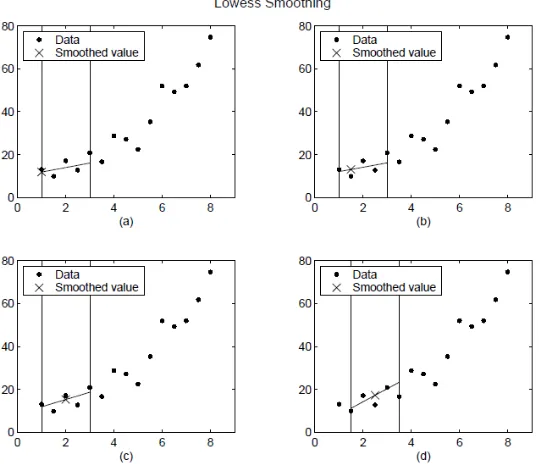
Figure 5. Lowess smoothing (a) and (b) use an asymmetric weight function, (c) and (d) use a symmetric weight function.
data point, the weight function is symmetric. However, if the number of neighboring points is not symmetric about the smoothed data point, then the weight function is not symmetric. Note that unlike the moving average
smoothing process, the span never changes. For example, when you smooth the data point with the smallest predictor value, the shape of the weight function is truncated by one half, the leftmost data point in the span has the largest weight, and all the neighboring points are
to the right of the smoothed value. The weight function for an end point and for an interior point is shown in Fig. 4 for a span of 31 data points. Using the lowess method with a span of five, the smoothed values and associated regressions for the first four data points of a generated data set are shown in Fig. 5(a) and (b) for an asymmetric
weight function use; Otherwise, (c) and (d) for symmetric weight function use.
5
For the loess method, the graphs would look the same except the smoothed value would be generated by a second-degree polynomial.
A. Robust Smoothing Procedure
If data contains outliers, the smoothed values can become distorted, and not reflect the behavior of the bulk of the neighboring data points. To overcome this problem, you can smooth the data using a robust procedure that is not influenced by a small fraction of outliers.
There is a robust version for both the lowess and loess smoothing methods. These robust methods include an additional calculation of robust weights, which is resistant to outliers. The robust smoothing procedure follows these steps [4].
1. Calculate the residuals from the smoothing procedure described in the previous section.
2. Compute the robust weights for each data point in the span. The weights are given by the bisquare function shown below.
where ri is the residual of the i-th data point produced
by the regression smoothing procedure, and MAD is the median absolute deviation of the residuals:
MAD = median( |r|)
The median absolute deviation is a measure of how spread out the residuals are. If ri is small compared to
6MAD, then the robust weight is close to 1. If ri is
greater than 6MAD, the robust weight is 0 and the associated data point is excluded from the smooth calculation
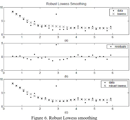
Figure 6. Robust Lowess smoothing
(a) outlier influences the smoothed value for several nearest neighbors; (b) residual of the outlier is greater than six median absolute deviations; (c) the smoothed values neighboring the outlier reflect the bulk of the
data.
3. Smooth the data again using the robust weights. The final smoothed value is calculated using both the local regression weight and the robust weight.
4. Repeat the previous two steps for a total of five the outlier is greater than six median absolute deviations. Therefore, the robust weight is zero for this data point. Plot (c) shows that the smoothed values neighboring the outlier reflect the bulk of the data.
B. Upper and Lower Smooths
The loess smoothing method provides a model of the middle of the distribution of Y given X. This can be extended to give us upper and lower smooths [7], where the distance between the upper and lower smooths
In this example, we generate some data to show how to get the upper and lower loess smooths. These data are obtained by adding noise to a sine wave. The resulting middle, upper and lower smooths are shown in Fig. 7, and we see that the smooths do somewhat follow a sine wave. It is also interesting to note that the upper and lower smooths indicate the symmetry of the noise and the constancy of the spread.
IV. KERNEL SMOOTHING METHODS
they fit the data in a local manner. These are called local
polynomial kernel estimators. We first define these
estimators in general and then present two special cases: the Nadaraya-Watson estimator and the local linear
kernel estimator.
With local polynomial kernel estimators, we obtain an estimate
y
0at a pointx
0by fitting a d-th degree polynomial using weighted least squares. As with loess, we want to weight the points based on their distance toFigure 7. The data for this example are generated by adding noise to a sine wave. The middle curve is the usual loess smooth, while the other curves are obtained using the upper and lower loess smooths.
0
x
. Those points that are closer should have greater weight, while points further away have less weight. To accomplish this, we use weights that are given by the height of a kernel function that is centered atx
0. As with probability density estimation, the kernel has a bandwidth or smoothing parameter represented by h. This controls the degree of influence points will have on the local fit. Ifh is small, then the curve will be wiggly, because the
estimate will depend heavily on points closest to
x
0. In this case, the model is trying to fit to local values (i.e., our ‘neighborhood’ is small), and we have over fitting. Larger values for h means that points further away will have similar influence as points that are close tox
0 (i.e., the ‘neighborhood’ is large). With a large enough h, we would be fitting the line to the whole data set.A. Nadaraya-Watson Estimator
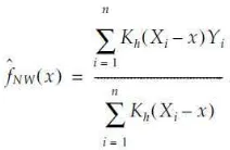
Some explicit expressions exist when d = 0 and d = 1. When d is zero, we fit a constant function locally at a given point . This estimator was developed separately by Nadaraya [9] and Watson [10]. The Nadaraya-Watson estimator is given below.
Note that this is for the case of a random design. When the design points are fixed, then the
X
i is replaced byi
x
, but otherwise the expression is the same [8]. The smooth from the Nadarya-Watson estimator is shown in Figure 8.Figure 8. Smoothing obtained from the Nadarya-Watson estimator with
h = 1.
There is an alternative estimator that can be used in the fixed design case. This is called the Priestley-Chao kernel estimator [11].
B. Priestley-Chao Estimator
The Priestley-Chao is given below.
where the
x
i,
i
=
1
,...,
n
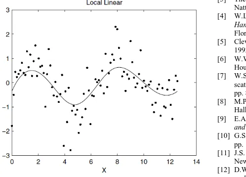
, represent a fixed set of ordered nonrandom numbers.C. Local Linear Kernel Estimator
When we fit a straight line at a point x, then we are using a local linear estimator. This corresponds to the case where d = 1, so our estimate is obtained as the
solutions
β
0andβ
1that minimize the following,7
where
As before, the fixed design case is obtained by replacing the random variable
X
iwith the fixed pointi
x
.When using the kernel smoothing methods, problems can arise near the boundary or extreme edges of the sample. This happens because the kernel window at the boundaries has missing data. In other words, we have weights from the kernel, but no data to associate with them. Wand and Jones [8] show that the local linear estimator behaves well in most cases, even at the boundaries. If the Nadaraya-Watson estimator is used, then modified kernels are needed ([8],[12]).
The local linear estimator is applied to the same generated sine wave data. The entire procedure is implemented and the resulting smooth is shown in Figure 9. Note that the curve seems to behave well at the boundary.
Figure 9. Smoothing obtained from the local linear estimator.
V. CONCLUSIONS
There are two common types of smoothing methods: filtering (averaging) and local regression. However, there are some methods which are arisen later, which can be classified as Kernel Smoothing, For which, now we can divide smoothing methods into three. Each smoothing method requires a span. The span defines a window of neighboring points to include in the smoothing calculation for each data point. This window moves across the data set as the smoothed response value is calculated for each predictor value. A large span increases the smoothness but decreases the resolution of the smoothed data set, while a small span decreases the smoothness but increases the resolution of the smoothed data set. The optimal span value depends on your data set and the smoothing method, and usually requires some experimentation to find.
REFERENCES
[1] W.S. Cleveland, Robust Locally Weighted Regression and
Smoothing Scatterplots, Journal of the American Statistical
Association, Vol. 74, pp. 829-836, 1979.
[2] http://www.itl.nist.gov/div898/handbook/pmd/section1/ pmd144.htm..
[3] The MathWorks, Curve Fitting Toolbox Users’ Guide, version 1, Nattick, MA, 2002.
[4] W.L. Martinez and A.R. Martinez, Computational Statistics
Handbook with Matlab, Chapman & Hall/CRC, Boca Raton,
Florida, 2002.
[5] Cleveland, W. S.. Visualizing Data, Hobart Press, New York, 1993
[6] W.W. Daniel and J.C. Terrell, Business Statistics, 5th edition,
Houghton Mifflin Company, Boston, 1989.
[7] W.S. Cleveland and Robert McGill, “The many faces of a scatterplot,” Journal of the American Statistical Association, 79: pp. 807-822, 1984.
[8] M.P. Wand and M. C. Jones, Kernel Smoothing, Chapman and Hall, London, 1995
[9] E.A. Nadaraya, “On estimating regression,” Theory of Probability
and its Applications, 10: pp. 186-190, 1964.
[10] G.S. Watson, “Smooth regression analysis,” Sankhya Series A, 26: pp. 101-116, 1964.
[11] J.S. Simonoff, Smoothing Methods in Statistics, Springer-Verlag, New York, 1996
[12] D.W. Scott, Multivariate Density Estimation: Theory, Practice,