Forensic.Speaker.Identification.eBook EEn

(1)

(2)

(3)

(4)

(5)

Taylor & Francis Forensic Science Series

Edited by James Robertson

Forensic Sciences Division, Australian Federal Police Firearms, the Law and Forensic Ballistics

T A Warlow ISBN 0 7484 0432 5 1996

Scientific Examination of Documents: methods and techniques, 2nd edition D Ellen

ISBN 0 7484 0580 1 1997

Forensic Investigation of Explosions A Beveridge

ISBN 0 7484 0565 8 1998

Forensic Examination of Human Hair J Robertson

ISBN 0 7484 0567 4 1999

Forensic Examination of Fibres, 2nd edition J Robertson and M Grieve

ISBN 0 7484 0816 9 1999

Forensic Examination of Glass and Paint: analysis and interpretation B Caddy

(6)

London and New York

Forensic Speaker

Identification

(7)

First published 2002 by Taylor & Francis 11 New Fetter Lane, London EC4P 4EE

Simultaneously published in the USA and Canada by Taylor & Francis Inc,

29 West 35th Street, New York, NY 10001

Taylor & Francis is an imprint of the Taylor & Francis Group

Typeset in Times by Graphicraft Ltd, Hong Kong

Printed and bound in Great Britain by TJ International Ltd, Padstow, Cornwall

All rights reserved. No part of this book may be reprinted or reproduced or utilised in any form or by any electronic, mechanical, or other means, now known or hereafter invented, including photocopying and recording, or in any information storage or retrieval system, without permission in writing from the publishers.

Every effort has been made to ensure that the advice and information in this book is true and accurate at the time of going to press. However, neither the publisher nor the author can accept any legal responsibility or liability for any errors or omissions that may be made. In the case of drug administration, any medical procedure or the use of technical equipment mentioned within this book, you are strongly advised to consult the manufacturer’s

guidelines.

British Library Cataloguing in Publication Data

A catalogue record for this book is available from the British Library

Library of Congress Cataloging in Publication Data A catalogue record has been requested

(8)

To my mum, who died on the day before she could see this book

finished.

(9)

Acknowledgements

In getting to the stage where I could even contemplate writing this book, and then actu-ally writing it, I have benefited from the help of many people, in many different ways. Now I can thank them formally for their contributions, which is a great pleasure. When I think of this book I think of the following people.

Hugh Selby, Reader in Law at the Australian National University. A long time ago, in commissioning a chapter on forensic speaker identification for his legal reference series Expert Evidence, Hugh introduced me to the Bayesian evaluation of evidence, with the implicit suggestion that I apply it to forensic speaker identification. Things seemed then to fall into place. How much is a key conceptual framework worth? That much I have to thank Hugh. Hugh also acted as my legal guinea-pig and read several early drafts, and he was also my source of information on legal matters. I also thank

Mie Selby, who was apparently never quite able to escape in time from having Hugh read some sections to her.

Dr Yuko Kinoshita, soon to be Lecturer in the School of Communication at the University of Canberra. Yuko gave me permission to use, in Chapter 11, a large por-tion of the results from her PhD research into forensic speaker identificapor-tion.

Dr Ann Kumar, Reader in Asian History at the Australian National University. Ann has contributed in several significant ways. She let me have some of her long Australian vowels for acoustic analysis in Chapter 8, and also compiled the glossary. Apart from reading and correcting several drafts, Ann was always there to listen to me try to formulate and express ideas, and offered continual encouragement. She said she found it very stimulating, and I’m sure it satisfied her intellectual curiosity. But I think she really should have been spending the time studying the comparative manufacture of Javanese Krises and Japanese ceremonial swords, or the agreement in mitochondrial DNA between Japanese and Indonesians. Now she can.

Drs Frantz Clermont and Michael ‘Spike’ Barlow of the Department of Computer Science at the University College of New South Wales. Frantz and Spike have been this poor linguistic phonetician’s window into the world of automatic speaker recognition. They also provided the superb if somewhat slightly extra-terrestrially disconcerting three-dimensional figure of the vocal tract tube in Chapter 6. Frantz has patiently tried to make the mathematics of the cepstrum understandable to me, without confusing me with what he says are its ‘dirty bits’. He spent a lot of his time creating the twoMatlab™ figures of the cepstrum in Chapter 8, and then getting them just right for me.

(15)

samples. As well as offering never-ending support and encouragement, Renata has been in total command of all the onerous background work and thus ensured that I have always been free to devote my time to writing. Unfortunately, unless I can do some really quick thinking, I now no longer have an excuse for not mowing the lawn.

Dr Francis Nolan, Reader in Phonetics at the University of Cambridge. As is obvious from the number of citations in the text, this book owes a tremendous intellectual debt to Francis’ extensive work on the phonetic bases of speaker recognition and its application to forensic phonetics. Francis also read an earlier draft and made many invaluable sug-gestions for improvement.

Alison Bagnall, Director of Voicecraft International. I have Alison to thank for making available the beautiful xero-radiographs of my vocal tract, and video of my vocal cords, which appear in Chapter 6. We made them at the (now) Women’s and Children’s Hospital in Adelaide, as part of an investigation for their marvellous cranio-facial unit into variation of vowel height and velopharyngeal port aperture.

My colleagues and students in the Linguistics Department at the Australian National University, and elsewhere. In particular, Professor Anna Wierzbicka, for her help with questions of semantic analysis; Professor Andrew Butcher, of the Department of Speech Pathology at Flinders University, South Australia, for encouragement and ideas and keeping me posted on his forensic-phonetic case-work in the context of many informative discussions on forensic speaker identification; Belinda Collins and Johanna Rendle-Short

for their help with conversation analysis; Jennifer Elliott for keeping me up-to-date with between-speaker and within-speaker variation in okay.

John Maindonald, formerly of the Statistical Consulting Unit of the Australian National University. John patiently fielded all my questions on statistical problems and then answered them again, and often again, when I still wasn’t quite sure.

James Robertson, head of forensic services for the Australian Federal Police. James was my series editor, and made many useful comments and corrections to drafts of several chapters of the book.

Len Cegielka, my eagle-eyed copy-editor. This book has greatly benefited from Len’s experienced and professional critique. I’m sure he is well aware of the considerable extent of his contribution, and doesn’t need me to tell him that he really has made a material improvement. So instead of that I will just express my thanks for a job very well done.

Professor Stephen Hyde in the Research School of Physical Sciences’ Department of Applied Mathematics at the Australian National University. Stephen contributed the 3-D figure in Chapter 2.

The book is ultimately the fault of Dr (now Pastor) Mark Durie, who was respons-ible for my embarking on forensic speaker identification. There have been times when I’m really not sure whether he actually deserves thanks for this.

All have given their knowledge and expertise to help make the book better, but also the most valuable thing of all: their time. They are in the happy, and deserved, position of partaking of all of the credit but none of the criticism. That, of course, is down to me alone.

(16)

government initiated a series of savage cuts by slashing 600 million dollars from the tertiary education budget. All the while incanting inane alliterations like ‘clever coun-try’ and ‘knowledge nation’, we are teaching less and less to more and more. Sadly, I don’t suppose this is much different from many other countries.

That modern master of the essay, Stephen Jay Gould recently wrote this about the current jeopardy of scholarly enquiry:

I just feel that the world of commerce and the world of intellect, by their intrinsic natures, must pursue different values and priorities – while the commercial world looms so much larger than our domain that we can only be engulfed and destroyed if we make a devil’s bargain of fusion for short-term gain.

Gould (2000: 26) Much the same sentiment is expressed in a recent P. D. James detective novel:

People who, like us, live in a dying civilisation have three choices. We can attempt to avert the decline as a child builds a sand-castle on the edge of the advancing tide. We can ignore the death of beauty, of scholarship, of art, of intellectual integrity, finding solace in our own consolations. . . . Thirdly, we can join the barbarians and take our share of the spoils.

James (2001: 380) Unfortunately, the person who wrote these pessimistic words in the novel is in fact the brutal murderer! Well, I too have often felt like murdering in the past few years, as change after change, cut after cut, has made it increasingly difficult to teach, to supervise, to do case-work and meaningful research, and to write this book.

The point I wish to make, however, is this. This book is about an aspect of applied scholarly endeavour, forensic phonetics, that carries with it very serious social re-sponsibilities. The book makes it clear that forensic speaker identification requires scholarly expertise, and in several disparate areas. Expertise, like forensically useful fundamental frequency, is a long-term thing. It requires an enormous amount of dedication on the part of students and teachers to get someone to the stage where they may responsibly undertake forensic case-work. This simply cannot be realised, in both senses of the term, under an ideology so clearly obsessed with the bottom line. Most people can learn to do a variety of things – I think the result is what is called multiskilling – but whether they will do them with sufficient skill and expertise is another matter. With the topic of this book that is precisely the question. It is about acquiring and exercising expertise. As Francis Nolan (1997: 767) has written: Justice will depend on it.

On a more optimistic note, then: I hope that this book will go a little way to helping all interested parties excel.

References

(17)

Gould, S. J. (2000) ‘The lying stones of Marrakech’, in Gould, S. J. The Lying Stones of Marrakech: Penultimate Reflections in Natural History: 9–26, London: Jonathan Cape. James, P. D. (2001) Death in Holy Orders, London: Faber and Faber.

(18)

Introduction

1 Introduction

Paul Prinzivalli, an air freight cargo handler in Los Angeles, stood trial for telephon-ing bomb threats to his employer, Pan Am. He was suspected because he was known to be a disgruntled employee, and because some Pan Am executives thought that the offender’s voice sounded like his. Defence was able to demonstrate with the help of forensic-phonetic analysis that the offender’s voice samples contained features typical of a New England accent, whereas Prinzivalli’s accent was unmistakably from New York. To untrained West Coast ears, the differences between New York and Boston accents are not very salient; to ears trained in linguistic and phonetic analysis, the recordings contained shibboleths galore. Reasonable doubt was established and Prinzivalli was acquitted (Labov and Harris 1994: 287–99).

In a case of the kidnapping and murder of an 11-year-old German girl (Künzel 1987: 5, 6), considerable agreement was found between the voice samples of a suspect and that of the kidnapper and, on the basis of this and other evidence, the suspect was arrested. Subsequently, a more intensive comparison between offender and suspect voice samples yielded yet more similarities. The man confessed during his trial.

In another American case involving a telephoned bomb threat (Hollien 1990: 51), the defendant had been identified by his voice. However, it was clear to forensic phon-eticians even from an auditory comparison that the voices of the defendant and the offender were very different. For example, the offender’s voice had features typical of someone who spoke English as a second language. The case was dismissed.

In the late 1990s in Australia, in a case concerning illegal drug trafficking (Q. vs. Duncan Lam 1999), police intercepted 15 incriminating telephone conversations con-taining 31 voice samples in Cantonese. Forensic-phonetic analysis was able to assign these 31 voice samples to three different speakers. Since the police, but not the analyst, knew the identity of some of the samples, not only could two of the speakers be identified, but the accuracy of the identification could also be checked.

(19)

could not be attributed to the suspect. A forensic-phonetic analysis was able to show that the brothers’ voices were distinguishable. Although their voices were indeed acous-tically very similar in many respects, they still differed in others, and in particular they both had different ways of saying their ‘r’ sound.

Forensic speaker identification

Expert opinion is increasingly being sought in the legal process as to whether two or more recordings of speech are from the same speaker. This is usually termed forensic speaker identification, or forensic speaker recognition. As the examples above show – and many more could be cited – forensic speaker identification can be very effective, contributing to both conviction and elimination of suspects. Equally importantly, the examples also demonstrate the necessity for expert evaluation of voice samples, since three of them show how the truth actually ran counter to the belief of naive listeners. Forensic speaker identification of the type described in this book – that is, using a combination of auditory and acoustic methods – has been around for quite a long time. Germany’s Bundeskriminalamt was one of the first institutions to implement it, in 1980 (Künzel 1995: 79), and the first conference on forensic applications of phon-etics was held in the United Kingdom in 1989. Yet there is still a considerable lack of understanding on the part of law enforcement agencies, legal practitioners, and indeed phoneticians and linguists, as to what it involves, what constitutes appropriate meth-odology, what it can achieve, and what its limitations are. In a 1995 Australian Court of Appeal report, for example, (Hayne and Crockett 1995: 2, 3) some perceived ‘weak-nesses in the science’ [of speaker identification] were explicitly listed, some of which were inaccurate (Rose 1996d). The aim of this book is to make explicit and explain in detail for the relevant professionals what is involved in forensic speaker identification (FSI), and to clarify the problems of inferring identity from speech under the very much less than ideal conditions typical in forensics.

Forensic phonetics

Forensic speaker identification is a part of forensicphonetics. Forensic phonetics is in turn an application of the subject of phonetics.Different experts have slightly differ-ing opinions on the exact subject matter of phonetics, and even whether it constitutes a discipline (Kohler 2000; Laver 2000; Ohala 2000). However, the following character-isation will not be controversial. Phonetics is concerned primarily with speech: it studies especially how people speak, how the speech is transmitted acoustically, and how it is perceived.

(20)

content identification and tape authentication, and only very indirectly with speaker profiling.

Readership

It is a good idea to be specific early on about the intended audience. I have had several types of readers in mind when writing this book. As just mentioned, I have written it to help members of the legal profession, the judiciary, and law enforcement agencies understand what forensic speaker identification is about. This will help them when requesting a forensic-phonetic investigation and help them understand and evaluate forensic-phonetic reports and evidence. I have also thought of linguistic phoneticians, budding and otherwise, who might be lured away from describing how languages differ phonetically to do valuable forensic-phonetic research into the complementary area of how their speakers differ. This book is also intended to be useful to those contemplating a professional career in forensic phonetics. I hope that the speech science community at large, including those working in the area of automatic speaker identification, will find much that is of use in the book. I hope, too, that the book will be accessible to both graduate and advanced undergraduate students in all related disciplines. Finally, I hope that the book will help stimulate the interest of statisticians who are thinking of researching, or supervising, forensic-statistical topics: there is especially much to be done in this area!

The take-home messages

The most important points that the book will make are these:

•

The forensic comparison of voice samples is extremely complex.

•

In the vast majority of cases the proper way to evaluate forensic speech samples, and thus to evaluate the weight of the forensic-phonetic evidence, is by estimating the probability of observing the differences between them assuming that the same speaker is involved; and the probability of observing the differences between them assuming that different speakers are involved. This method is thus inherently probabilistic, and as such will not yield an absolute identification or exclusion of the suspect.

•

The two main problems in evaluating differences between samples are (1) dif-ferential variation in voices, both from the same speaker and from different speakers, and (2) the variable and generally poor degree of control over forensic speech samples.

•

Speech samples need to be compared both acoustically and auditorily, and they also need to be compared from the point of view of their linguistic and non-linguistic features.

(21)

Argument and structure of the book

Speaker identification in the forensic context is usually about comparing voices. Probably the most common task involves the comparison of one or more samples of an offender’s voice with one or more samples of a suspect’s voice. Voices are important things for humans. They are the medium through which we do a lot of communicat-ing with the outside world: our ideas, of course, but also our emotions and our personality:

The voice is the very emblem of the speaker, indelibly woven into the fabric of speech. In this sense, each of our utterances of spoken language carries not only its own message, but through accent, tone of voice and habitual voice quality it is at the same time an audible declaration of our membership of particular social regional groups, of our individual physical and psychological identity, and of our momentary mood.

Laver (1994: 2) Voices are also one of the media through which we (successfully, most of the time) recognise other humans who are important to us – members of our family, media personalities, our friends and enemies. Although evidence from DNA analysis is poten-tially vastly more eloquent in its power than evidence from voices, DNA can’t talk. It can’t be recorded planning, carrying out or confessing to a crime. It can’t be so apparently directly incriminating. Perhaps it is these features that contribute to the interest and importance of FSI.

As will quickly become evident, voices are extremely complex things, and some of the inherent limitations of the forensic-phonetic method are in part a consequence of the interaction between their complexity and the real world in which they are used. It is one of the aims of this book to explain how this comes about.

Because of the complexity of the subject matter, there is no straightforward way to present the information that is necessary to understand how voices can be related, or not, to their owners. I have chosen to organise this book into four main parts:

•

The first part, in Chapters2–5, introduces the basic ideas in FSI: Why voices are difficult to discriminate forensically, Forensic-phonetic parameters, Expressing the outcome, Characterising forensic-phonetic speaker identification.

•

The second part, Chapters 6–9, describes what speech sounds are like: The human vocal tract and the production and perception of speech sounds, Phonemics, Speech acoustics, Speech perception.

•

The third part, in Chapter 10, describes what a voice is.

•

The fourth part, in Chapter 11, demonstrates the method using forensically real-istic speech.

(22)

come. Thus, for example, it is difficult to understand how speakers differ in phonemic structure without understanding phonemics in Chapter 7, and very difficult to under-stand phonemics without a prior underunder-standing of speech sounds from Chapter 6.The demonstration of the method in Chapter 11 will be much easier to understand with knowledge of speech acoustics in Chapter 8.

Because this book is intended to be of use to so many disparate groups, I have adopted an inclusive approach and erred on the side of detail. This means that some readers may find more detail in some chapters than they need. I can imagine that members of the legal profession will not be able to get quite as excited as I do about formant frequencies, for example, and readers with some background knowledge of articulatory phonetics do not need to learn about vocal tract structure. Feel free to skip accordingly, but please be aware of the cumulative structure of the book’s argument.

A brief characterisation of the contents now follows.

Basic ideas

In Chapters 2 to 5 are introduced the ideas that are central to the problem of FSI. There are four themes, one to each chapter. The first theme, in Chapter 2, describes what it is about voices that makes FSI difficult. This includes the existence of within-speaker as well as between-within-speaker variation, and its consequences for discriminating between speakers; what conditions variation, and our lack of control over it in the real world. The second theme, in Chapter 3, is forensic-phonetic parameters. Here are dis-cussed the different types of parameters used to compare speech samples forensically. The third theme describes the proper conceptual framework and way of expressing the outcome of a forensic-phonetic identification. This is in Chapter 4. The fourth theme, in Chapter 5, shows how FSI relates to other types of speaker recognition.

What speech sounds are like

FSI is performed on recordings of human vocalisations – sounds made exclusively by a human vocal tract. Although other vocalisations, for example laughs or screams, may from time to time be forensically important (Hirson 1995), most of the vocalisations used in FSI are examples of speech. Speech is the primary medium of that supremely human symbolic communication system called Language. One of the functions of a voice – perhaps the main one – is to realise Language, by conveying some of the speaker’s thoughts in linguistic form. Speech is Language made audible.

Moreover, when forensic phoneticians compare and describe voices, they usually do so with respect to linguistic units, especially speech sounds, like vowels or consonants. They might observe, for example, that the ee vowels in two samples are different; or that the th sound is idiosyncratically produced in both. It is therefore necessary to understand something of the structure of speech sounds, and how they are described. A large part of this book, Chapters 6 to 9, is accordingly given over to a description of the nature of speech sounds.

(23)

Chapter 7 (Phonemics) is concerned with how speech sounds are functionally organised in language. Phonemics is a conceptual framework that the forensic description of speech sounds usually assumes, and within which it is conveniently, and indeed indispensably, presented.

Phonemics regards actual speech sounds (called phones) as realisations of abstract sounds, called phonemes, whose function is to distinguish words. Thus the vowel in the word bead, and the vowel in the word bid are said to realise different phonemes in English because the phonetic difference between them – one vowel is, among other things, shorter than the other – signals a difference between words. The consonant sounds at the beginning of the words red and led realise different phonemes for the same reason. Phonemics is indispensable, because it supplies the basis for comparison of speech sounds in the first place. It allows us to say, for example, that two speech sounds are potentially comparable across samples because they are realisations of the same phoneme. This would enable us to legitimately compare, acoustically and phon-etically, the vowel in the word car in one sample, say, with the vowel in the word farin another, because they are realisations of the same phoneme.

It is generally assumed that similarities and differences between forensic speech samples should be quantified acoustically, and acoustic comparison is an indispensable part of forensic-phonetic investigation. It is therefore necessary to describe speech acoustics, especially those that are assumed to be the ones in which speaker identity is optimally encoded. Speech acoustics are described in Chapter 8.

Several aspects of speech perception – how humans decode the speech acoustics to hear speech – are relevant for forensic phonetics. In particular, one argument for the necessity of analysing forensic speech samples both auditorily and acoustically is based on speech perception. It is also important to know about the expectation effect (you hear what you expect to hear), another aspect of speech perception. Both are discussed in Chapter 9: Speech perception.

The contents of Chapters 6 to 9, then, describe some of the basic knowledge that informs phonetic work. For example, it would be typical for a forensic-phonetic expert to listen to two speech samples, decide what is comparable in terms of occurrences of the same phoneme, describe and transcribe the phonemes’ realisations, and then quantify the differences acoustically.

(24)

These aims have their downside. It would be silly to pretend that all of the specialist topics I have tried to explain in some detail are easy. They are quite definitely not, and the reader must be prepared to find at least some of the chapters difficult. Like many difficult passages, however, they become much more understandable on repeated readings.

What is a voice?

A voice is more than just a string of sounds. Voices are inherently complex. They signal a great deal of information in addition to the intended linguistic message: the speaker’s sex, for example, or their emotional state or state of health. Some of this information is clearly of potential forensic importance. However, the different types of information conveyed by a voice are not signalled in separate channels, but are convolved together with the linguistic message. Knowledge of how this occurs is neces-sary to interpret the ubiquitous variation in speech, and to assess the comparability of speech samples.

Familiar things like voices we tend to take for granted. In this case familiarity breeds false understanding. We assume they are simple, and that we know about them. This is especially typical for language, and phenomena that are intimately connected with language (Lyons 1981: 38). Language is absolutely fascinating, and nearly every-one has an unreflected opinion on aspects of their own language. Although not all languages have a separate word for voice, all languages have words for describing the way speakers sound when they talk: in English, for example, they can be harsh, kind, sexy, masculine, gruff, melodious, sibilant, booming, staccato, etc. (Laver 1991f ).

A voice is, however, an extremely complex object, and a large part of this complexity lies in its relationship with its owner. When comparing voices, it is imperative that one knows about what one is comparing. Consequently, it is very important to have a model for the information content in a voice, and how these different components inter-relate and interact. A model for the voice is presented in Chapter 10: What is a voice?

The likelihood ratio revisited: a demonstration of the method

A book like this could obviously not be taken seriously if it could not demonstrate that the method worked – that forensically realistic speech samples from the same speaker can be distinguished from speech samples from different speakers. In Chap-ter 11, then, will be found such a demonstration, together with an explanation of the basic mechanics of the statistical approach used (called the likelihood ratio), and its shortcomings.

Chapter 12 contains a summary of the book, and addresses questions of what, in terms of data, method, and qualifications of practitioner, constitutes the requirements for a successful forensic speaker identification. It also asks what developments can be expected in the future.

(25)

Why voices are difficult to discriminate forensically

2 Why voices are difficult to

discriminate forensically

As flagged in the introduction, the aim of this and the following three chapters is to introduce in as non-technical way as possible ideas and distinctions that are central to the understanding of forensic speaker identification. In this chapter I describe what it is about voices that makes identifying them or telling them apart under realistic forensic conditions problematic.

Probably the most common task in forensic speaker identification involves the comparison of one or more samples of an unknown voice (sometimes called the ques-tioned sample(s) ) with one or more samples of a known voice. Often the unknown voice is that of the individual alleged to have committed an offence (hereafter called the offender) and the known voice belongs to the suspect. Both prosecution and defence are then concerned with being able to say whether the two samples have come from the same person, and thus being able either to identify the suspect as the offender or to eliminate them from suspicion. Sometimes it is important to be able to attach a voice to an individual, or not, irrespective of questions of guilt.

In order to tell whether the same voice is present in two or more speech samples, it must be possible to tell the difference between, or discriminate between, voices. Put more accurately, it must be possible to discriminate between samples from the voice of the same speaker and samples from the voices of different speakers (Broeders 1995: 158). So identification in this sense is the secondary result of a process of discrimina-tion. The suspect may be identified as the offender to the extent that the evidence supports the hypothesis that questioned and suspect samples are from the same voice. If not, no identification results. In this regard, therefore, the identification in forensic speaker identification is somewhat imprecise. However, since the term identification is commonly found (recognition is another common term), I have chosen to use it in this book. It can also be noted here that the word discrimination is usually used in a sense that differs somewhat from that just described. This point will be taken up later.

(26)

conditions normally present in forensic case work. One of the aims of this chapter is therefore to clarify the reasons for this – why discrimination becomes more problem-atic in the real world of forensic phonetics.

It stands to reason that if entities are to be discriminated by one of their attributes, those entities must differ in that attribute. If everyone had the same voice, voices would be no use for discrimination. Thus, if individuals are to be discriminated by their voices, individuals must differ in their voices. They do, but the voice of the same speaker can also show considerable variation. This variation must now be discussed.

Between-speaker and within-speaker variation

Under ideal conditions, speakers can be identified reasonably easily by their voices. We know this from the excellent performance of automated speaker recognition sys-tems (to be discussed below). And we probably suspected it already because we have all had the experience of hearing identity: we humans recognise familiar voices, fairly successfully, all the time. This probably entitles us to assume that different speakers of the same language do indeed have different voices, although as already foreshadowed the extent to which this can be assumed forensically is a separate issue. We thus have to deal with variation between speakers, usually known as between-speaker (or inter-speaker) variation.

Although it is a general assumption that different speakers have different voices, it is crucial to understand that the voice of the same speaker will always vary as well. It is a phonetic truism that no-one ever says the same thing in exactly the same way. (For a demonstration of some of the acoustic differences that occur between repeats of the same word, see Rose 1996a). It is therefore necessary to come to terms with variation within a speaker. This is usually termed within-speaker or intra-speaker variation. (The latter term, with intra-, sounds confusingly similar to the inter- of inter-speaker varia-tion and, as I also always have trouble in remembering which is which, is accordingly avoided in this book.)

Probably the most important consequence of this variation is that there will always be differences between speech samples, even if they come from the same speaker. These differences, which will usually be audible, and always measurable and quantifiable, have to be evaluated correctly if forensic speaker identification is to work. To put it another way, forensic speaker identification involves being able to tell whether the inevitable differences between samples are more likely to be within-speaker differences or between-speaker differences.

Given the existence of within-speaker variation, it is obvious that the other logical requirement on the feasibility of forensic speaker identification (or indeed any identi-fication system) is that variation between speakers be bigger than the variation within a speaker. Again, this appears to be the case: providing that one looks at the right things, there is greater variation between the voices of different speakers than within the voice of the same speaker. It is also intuitively obvious that the greater the ratio of between-speaker to within-speaker variation, the easier the identification.

(27)

Figure 2.1 Three speakers in one dimension

pitch would then be termed a dimension. (Other commonly found synonyms are parameter, or feature.) In the figure, ‘5’ marks a particular value within this dimen-sion (or parameter, or feature). For the moment, let us assume that these values were measured from the speakers on one particular occasion: perhaps measurements were taken once at the beginning and end of their speech, once in the middle, and twice somewhere in-between, thus making five measurements per speaker. (Measurements are often referred to as observations, and the terms are used interchangeably in this book.)

Figure 2.1 shows how speakers vary along the single ‘average pitch’ dimension – speaker B’s lowest value is 110 ‘average pitch’ units, for example. It can be seen firstly that there is between-speaker variation: each speaker has different values for the dimension. Within-speaker variation is also evident: each speaker is characterised by a set of different values for the dimension. It can also be seen that variation within a speaker for the ‘average pitch’ dimension is small compared to the variation between speakers. For example, the largest difference between two observations for the same speaker is smaller than the smallest difference between any two speakers.

It can be appreciated that, given this kind of distribution, if we take any two values for this dimension, it would be easy to correctly discriminate them – to say whether the two values had come from the same speaker or not. If we took values of 100 and 104, for example, we could say that they came from the same speaker; if we took 100 and 110, we could say they came from different speakers. The reader might like to formulate the discriminant function for these data: the condition under which any two observations could be said to come from different speakers.1

(28)

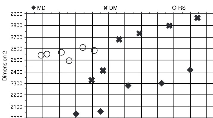
Figure 2.2 Three speakers with overlapping values in one dimension

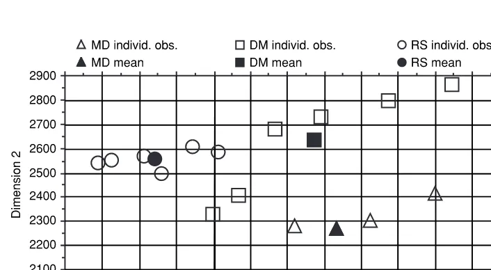
In reality, however, speakers overlap in their distributions for a dimension. Some-times they overlap a little, someSome-times a lot, and someSome-times completely. This situation is illustrated in Figure 2.2, which, in contrast to the made-up data in Figure 2.1, now shows real data from three speakers: MD, DM, RS. The dimension involved is an easily measured acoustic value in the second syllable of the word hello (the data are from Rose 1999a). Six hellos from each of the three speakers were measured, and the values plotted in the figure (their unit is hertz, abbreviated Hz). It can be seen that the speaker with the lowest observation was RS, whose lowest value was about 1240 Hz. The highest value, of about 1800 Hz, belongs to speaker MD.

The most important feature of Figure 2.2 is that the speakers can be seen to over-lap. Speakers MD and DM overlap a lot: DM’s range of values is from 1399 Hz to 1723 Hz, and is covered completely by MD, whose range is from 1351 Hz to 1799 Hz. Speaker RS, whose range is from 1244 Hz to 1406 Hz, encroaches a little on the lower ends of the other two speakers’ ranges.

The consequences of this overlapping are drastic. Now it is no longer possible to give a value for magnitude of difference between samples that will always correctly discriminate between the same and different speakers. This is because the smallest dif-ference between two different speakers, e.g. the difdif-ference of 7 Hz between DM’s lowest value of 1399 Hz and RS’s highest value of 1406 Hz, is smaller than the smallest within-speaker difference. Therefore, although we could say that a difference between any two observations that is greater than 448 Hz always indicates different speakers (because 448 Hz is the biggest within-speaker difference between the lowest and highest observations in the data) we cannot stipulate a threshold, values smaller than which will always demonstrate the presence of the same speaker.

(29)

discriminated. For example, if we chose a threshold value of 150 Hz, such that differ-ences between paired observations greater than 150 Hz were counted as coming from different speakers, and differences smaller than 150 Hz counted as the same speaker, we could actually correctly discriminate about 60% of all 153 pairs of between-speaker and within-speaker comparisons. (With six tokens each from three speakers, there are 45 possible within-speaker comparisons; and 108 possible between-speaker compar-isons.) For example, the difference of 35 Hz between speaker RS’s highest value of 1406 Hz and his next highest value of 1371 Hz is less than 150 Hz, and is therefore cor-rectly discriminated as a within-speaker difference. Likewise the difference of 155 Hz between RS’s lowest value of 1244 Hz and DM’s lowest value of 1399 would be correctly discriminated ( just!) as a between-speaker difference. However, the difference between RS’s highest value of 1406 and his lowest value of 1244 Hz is greater than 150 Hz and would be incorrectly classified as coming from two different speakers. This would count as a false negative: deciding that two observations come from different speakers when in fact they do not.

More significantly, the difference between RS’s highest value of 1406 and DM’s lowest value of 1399 Hz will be incorrectly discriminated as coming from the same speaker. This would count as a judicially fatal false positive: DM, assuming he is the accused, is now convicted of the crime committed by RS.

If we choose this threshold (of 150 Hz), then we get about the same percentage of between-speaker comparisons incorrect as within-speaker comparisons. This is called an equal error rate (EER); since we get about 60% correct discriminations, the EER in this case will be about 40%.

The threshold can, of course, be set to deliver other error rates. If we wished to ensure that a smaller percentage of false positives ensue (samples from two different speakers identified as coming from the same speaker), then we set the threshold lower. This would, of course, have the effect of increasing the instances where the real offender is incorrectly excluded.

Where does the figure of 150 Hz for the equal error rate threshold come from? It can be estimated from a knowledge of the statistical properties of the distribution of within-speaker and between-speaker differences, or it can be found by trial and error by choosing an initial threshold value, noting how well it performs, and adjust-ing it up or down until the desired resolution, in this case the equal error rate, is achieved.

Probabilities of evidence

The typical fact that only a certain percentage of cases can be correctly discriminated – for these data 60% – is another consequence of the overlap, and introduces the necessity for probability statements. For example, we would expect that a decision based on the application of the ‘150 Hz threshold’ test to any pair of observations from the above data would be correct 60% of the time and incorrect 40% of the time.

(30)

difference between two observations assuming that they come from the same speaker (60%), and assuming they come from different speakers (40%). Note that it is the probabilities of the evidence as provided by the test that are being given here and not the probability of the hypothesis that the same speaker is involved. This thus gives us a measure of the strength of the test. In other words, whatever our estimate was of the odds in favour of common origin of the two samples before the test, if the two observations are separated by less than 150 Hz, we are now 60/40 = one and a half times more sure that they do have a common origin. And if they are separated by more than 150 Hz, we are one and a half times more sure that they do not. Not a lot, to be sure, but still something.

Note that this also introduces the notion of probability in the sense of an expecta-tion, or as a measure of how much we believe in the truth of a claim (here, that the two observations come from the same speaker). The importance of assessing the probabilities of the evidence and not the hypothesis is a central notion and will need to be addressed in detail in Chapter 4.

Distribution in speaker space

The three speakers’ monodimensional data in Figure 2.2 also illustrate two more important things about voices. It is possible to appreciate that RS differs from MD and DM much more than the latter two differ. This is illustrative of the fact that voices are not all distributed equally in speaker space: some are closer together than others. This could also possibly be guessed from the fact that some voices sound more similar than others. Not so easy to guess is the fact that speakers can differ in the amount by which they vary for a dimension. This is also illustrated in Figure 2.2, where it can be seen that RS’s individual observations distribute more compactly than DM’s and MD’s. The fact that speakers vary in their variability is an additional complica-tion in discriminacomplica-tion.

The unequal distribution of voices is one reason why our illustrative discrimination, with its ‘average equal error rate’, is unrealistic. It will not be the case that all pairs of speakers will be discriminable to the same extent, because a small amount of really good discrimination between speakers who are well separated in speaker space, for example between RS and DM, or between RS and MD, can cancel out a large amount of poor discrimination, for example between MD and DM. This means that an average equal error rate can be misleading. It is because of this that sophisticated statistical techniques, for example linear discriminant analysis, are required to give a proper estimate of the inherent discriminating power of dimensions.

Multidimensionality

(31)

Figure 2.3 Three speakers in two dimensions

Two-dimensional comparison

Figure 2.3 shows the same three speakers as Figure 2.2, this time positioned with respect to two dimensions. The original dimension from Figure 2.2 is retained on the horizontal axis, and another acoustical dimension, this time having to do with the ‘l’ sound in the word hello, and also quantified in Hz, is shown vertically.

Now it can be seen that, although DM and MD largely overlap along the first dimension, they overlap much less on the second: DM’s lowest value is 2328 Hz, MD’s highest value is 2509, and two of DM’s values lie within MD’s range. RS’s values, which have a narrower distribution in the second dimension than the other two, are overlapped completely by DM and only minimally by MD.

As a result of quantifying speakers with respect to these two dimensions, the speakers can be seen to occupy more different positions in two-dimensional than one-dimensional speaker space.

It should be clear that, if it is possible to take into account differences in two dimensions, and the dimensions separate out speakers a little, there is the possibility of achieving a better discrimination than with a single dimension. This can be demon-strated with the data in Figure 2.3.

(32)

√(1244 − 1262)2₊₍₂₅₄₃₋₂₅₅₆₎2 =√(−18)2₊

(−13)2 =√(324) + (169) =√493

= 22.2

It can be seen from Figure 2.3 that there are still many different-speaker pairs that are separated by about the same amount as same-speaker pairs. Nevertheless, the overall greater separation results in a slight improvement in discrimination power (Aitken 1995: 80–2). Now about 70% of all 153 pairs can be discriminated, compared to 60% and 62% with the first and second single dimensions respectively. An improvement in discrimination performance will only happen if the dimensions are not strongly corre-lated, otherwise the same discrimination performance occurs with two well-correlated dimensions as with one. For the data in Figure 2.3, it can be seen that there is in fact a certain degree of correlation, since the second dimension increases as the first in-creases. The question of correlation between dimensions is an important one, to be examined in greater detail later.

Figure 2.3 shows two configurations typical for voice comparison: that one pair of speakers can be well separated in dimension 1 but not in dimension 2, whereas another pair might be well separated in dimension 2 but not in dimension 1. The other two logical possibilities are also found: that a pair of speakers can be well separated in both dimensions, and not separated in either dimension. Note that the second dimension in Figure 2.3, just like the first, will not correctly separate out all three speakers: there is no single dimension that will correctly discriminate all speakers.

Multidimensional comparison

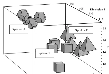
It is of course possible, theoretically, to carry the comparison to as many dimensions as desired. (The Euclidean distance between two observations in three dimensions now becomes the square-root of the sum of the squares of the differences between the observations in all three dimensions.) Figure 2.4 gives an idea of how three speakers might position in three-dimensional space (different dimensions and values are used from the previous examples).

(33)

Figure 2.4 Three speakers in three dimensions

Discrimination in forensic speaker identification

In forensic speaker identification, then, the task is to discriminate between same-speaker voice samples and different-same-speaker voice samples. It was observed earlier in this chapter that this is using the word discrimination in a somewhat different sense from that encountered generally in statistics. The difference between the two senses is important and is explained here.

The way discrimination is usually construed in statistics – let us call this classical discriminant analysis – can be illustrated once again using data from the three speakers in Figure 2.3. A typical classical discriminant analysis on these three speakers would involve deriving a discriminant function from the existing data, such that any new tokens from any of the three speakers could be correctly attributed to the correct speaker. For example, we might take another of DM’s hellos, find that it measured 1575 Hz on dimension one, and 2650 Hz on dimension two. The discriminant function that had been established with the old data would then hopefully identify this new token as having come from DM. It can be seen that an identification is involved here: the new token is identified by classical discriminant analysis as belonging to DM.

(34)

Classical discrimination is clearly useful for finding out whether a particular dimen-sion might be of use in forensic speaker identification, and there are many experi-ments in the literature where discriminant analysis of this type is used to demonstrate that a certain set of dimensions can correctly discriminate a predetermined set of speakers. However, it is of limited applicability in circumstances typical of forensic speaker identification. This is because in forensic speaker identification one does not normally have a predetermined set of known individuals to which the questioned sample is to be attributed on the basis of a set of dimensions. All one has is two (sets of) samples: questioned and suspect, and one does not know (of course!) whether the suspect’s voice is the same as that of the offender.

If one wants to look at the problem from the point of view of discriminant analysis, only two categories are involved in forensic speaker identification: same-speaker pairs and different-speaker pairs. The task is then to examine the pair of samples from offender and suspect and determine to what extent the evidence supports whether the pair is to be attributed to the category of same-speaker pair or different-speaker pair. It is part of the aim of this book to show that this can be done, and how it is done.

Dimensional resolving power

Although a speaker’s voice can be characterised in many different dimensions, not all dimensions are equally powerful. They vary according to their discriminatory power. For example, the discriminating power of the first dimension in Figure 2.3 on its own was 60%, whereas that of the second was 62%. Obviously, it is of no use to compare samples along dimensions that have little or no resolving power, and it is part of gen-eral forensic-phonetic knowledge to know which are the more powerful dimensions. This is a very important point, since time is usually limited and cannot be wasted on comparing samples with respect to weak dimensions.

The most powerful dimensions are naturally those that show a small amount of variation within a speaker and a large amount of variation between speakers, so a common way of selecting potentially useful forensic speaker identification dimensions has been to inspect the ratio of between-speaker to within-speaker variation (Pruzansky and Mathews 1964; Wolf 1972; Nolan 1983: 101; Kinoshita 2001). This ratio is called the F-ratio, and is usually a by-product of a statistical procedure called Analysis of Variance or ANOVA (‘ann-over’) (the proper statistical term for variation in this sense is variance). The discriminant power of the dimensions is then determined in discrimin-ant analyses, as mentioned above.

The reader should now be able to understand that it is always important to estab-lish that any dimension that is being used to compare speakers forensically is known to show at least greater between-speaker variation than within-speaker variation.

Ideal vs. realistic conditions

(35)

So far, all of this applies to any speaker recognition system. However, it is import-ant to understand that there are very big differences between speaker recognition under ideal conditions and forensic speaker identification, where the real-world circum-stances make conditions very much less than ideal. This is of course the individuality postulate in another guise, whereby no two objects (here: speakers’ voices) are identical, although they may be indistinguishable (Robertson and Vignaux 1995: 4). These less than ideal conditions make forensic speaker identification difficult for the following two reasons: lack of control over variation, and reduction in dimensions for comparison. These will now be discussed.

Lack of control over variation

It was pointed out above that variation is typical of speech, and that there is variation both between and within speakers. Some of the variation in speech is best understood as random, but a lot of it can be assumed to be systematic, occurring as a function of a multitude of factors inherent in the speech situation. For example, between-speaker variation in acoustic output occurs trivially because different speakers, for example men and women, have vocal tracts of different dimensions (why this is so is explained in Chapter 6). Within-speaker variation might occur as a function of the speaker’s differing emotional or physical state.

Since we usually do not have total control over situations in which forensic samples are taken, this is one major problem in evaluating the inevitably occurring differences between samples. This point is so important that it warrants an example. A concrete, but simplified, example with our ‘average pitch’ dimension will make this clear.

Let us assume that some speakers differ in the pitch of their voice. The pitch dif-ference, which can be heard easily between men’s and women’s voices, also exists between speakers of the same sex, and is due to anatomical reasons connected with the size and shape of the vocal cords, which are responsible for pitch production.

However, the pitch of a speaker also varies as a function of other aspects of the situation. These will include, but not exhaustively: the speaker’s mood, the linguistic message, and their interlocutor. The pitch can change as a function of the speaker’s mood: it might be higher, with a wider range, if the speaker is excited; lower, with a narrow range if they are fed-up. The speaker’s pitch will also change as a function of the linguistic message. In English it will normally rise, and therefore be higher, on questions expecting the answer yes or no. (Try saying ‘Are you going?’ in a normal tone of voice, and note the pitch rise on going.)

(36)

patterns. One subject of a recent forensic-phonetic investigation has been observed using an r sound after their vowels in words like car and father when speaking with inmates of an American prison, but leaving the postvocalic r sounds out when speak-ing with Australians (J. Elliott, personal communication). This behaviour suggests that he was accommodating to either real or perceived features in his interlocutors’ voices. This is because one of the ways in which most (but not all) varieties of Amer-ican English differ from Australian English is in the presence vs. absence of post-vocalic r.

Imagine a situation where an offender is recorded on the video surveillance system during an armed hold-up. The robber shouts threats, is deliberately intimidating: their voice pitch is high, with a narrow range. A suspect is interviewed by the police in the early hours of the morning. He almost certainly feels tired, and perhaps also alien-ated, intimidalien-ated, cowed and reticent. As a result, if he says anything useful at all, his pitch is low, with a small range. Although the pitch difference between the questioned and suspect samples will almost certainly be bigger than that obtaining between some different speakers, it cannot be taken to exclude the suspect, because of the different circumstances involved.

Now imagine a situation where an offender with normally high pitch is perpetrating a telephone fraud. The suspect, who has a normally low-pitched voice, is also inter-cepted over the telephone talking to their daughter: they are animated, congenial, happy: their pitch is high, and very similar to that of the offender. Although the observed pitch difference between the samples is less than that which is sometimes found within the same speakers, it cannot be taken as automatically incriminatory because of the different circumstances involved.

Individuals’ voices are not invariant but vary in response to the different situations involved. Depending on the circumstances, this can lead to samples from two different speakers having similar values for certain dimensions; or samples from the same speaker having different values for certain dimensions. It is also to be expected that samples from the same speaker will be similar in certain dimensions, and samples from different speakers will differ in certain dimensions.

Differences between voice samples, then, correlate with very many things. The differences may be due to the fact that two different speakers are involved; or they may reflect a single speaker speaking under different circumstances – with severe laryngitis, perhaps, on one occasion and in good health on another. One common circumstance that is associated with within-speaker variation is simply the fact that a long time separates one speech sample from another: there is usually greater within-speaker variation between samples separated by a longer period of time than between speech samples separated by a short period (Rose 1999b: 2, 25–6).

The effect of all this will be to increase the variation, primarily within speakers, and thus reduce the ratio of between-speaker to within-speaker variance of dimensions. This will result in a decrease in our ability to discriminate voices.

(37)

to suggest that this is so (Hirson et al. 1995), a higher pitch for the phone voice will be expected and not be exclusionary. However, a lower pitch for the telephone voice, or perhaps even the same pitch, will suggest an exclusion of the suspect.

In order to be able to evaluate all this, we need to know about how voices differ in response to different circumstances. Situations also need to be comparable with respect to their effect on speech. There may be situations where it is not possible to compare forensic samples because the effect of the situations in which they were obtained is considered to be too different. This basic comparability is one of the first things that a forensic phonetician has to decide.

Reduction in dimensionality

The second effect of the real-world context on forensic speaker comparison is a sub-stantial reduction in dimensionality of the voices to be compared. This commonly occurs in telephone speech, for example, where dimensions that may be of use – that is dimensions with relatively high resolution power – are simply not available because they have been filtered out. It can also occur as the result of many other practical factors, like noisy background, someone else speaking at the same time, and so on.

A not insignificant factor in this respect is time (Braun and Künzel 1998: 14). The identification, extraction, and statistical comparison of speech dimensions take a lot of time, especially for investigators who are not full-time forensic phoneticians. Whereas the enlightened governments of some countries, e.g. Holland, Germany, Sweden, Austria, Spain and Switzerland, employ full-time forensic phoneticians, in others, e.g. Australia and the United Kingdom, a lot of this work is done by academic phon-eticians who already have heavy research, teaching, supervisory and administrative loads. Time might therefore simply not be available to compare samples with respect to all important dimensions. Since our ability to discriminate voices is clearly a func-tion of the available dimensions, any reducfunc-tion in the number of available dimensions constitutes a limitation.

In addition to reduction, distortion of dimensions is a further problem associated with the real world. This occurs most commonly in telephone transmission (Rose and Simmons 1996; Künzel 2001). For example, the higher values of the second dimension that I adduced in Figure 2.3 to improve discrimination would in all probability be compromised by a bad telephone line. Distortion can also result from inadequate recording conditions, a low-quality tape recorder and/or microphone, echoic rooms, etc. Again, it is necessary to know what the effects are on different dimensions, and which dimensions are more resistant to distortion.

An interesting point arises from this practically imposed reduction in dimensionality. As a result, dimensions in which samples from different speakers differed a lot could be excluded. Then samples from two voices that in reality differed a lot would appear not to differ so much.

(38)

different, whereas there is no upper limit on the amount by which two samples can differ. There thus exists an asymmetry in the distribution of differences between samples, with a wall of minimal differences. (For a useful discussion on the effect of the wall phenomenon see Gould (1996, esp. ch.13) ).

At first blush, this sounds like good news for defence. It looks as though it could be argued that, although two samples do not differ very much, they may still be from different speakers, since it is possible that the dimensions strongly differentiating the speakers were not available for comparison. Moreover, a mutatis mutandis argument – although there are large differences between the voice samples, they still come from the same speaker – is clearly not available to the prosecution.

Such a defence argument is, in fact, logically possible if discussion is confined to differences between samples. As will be demonstrated in detail below, however, dis-cussion cannot be thus restricted, since the magnitude of differences between samples constitutes only half the information necessary to evaluate the evidence: it will be shown below that the question of how typical the differences are is equally important for its evaluation.

Representativeness of forensic data

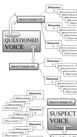
A final way in which real-world conditions make it difficult to forensically discrim-inate speakers has to do with the representativeness of the data that are used to compare voices forensically. By representativeness is meant how representative the actual observations are of the voice they came from. The more representative the data are of their voices, the stronger will be the estimate of the strength of the evidence, either for or against common origin. Below we examine the main factors influencing the representativeness of forensic speech data. First, however, it is necessary to outline a model showing how typical forensic speaker identification data are structured. This model is shown in Figure 2.5.

Typically, speech samples in forensic speaker identification come from two sources. One source is the voice of the offender. The other is the voice of the suspect. These two sources are marked in Figure 2.5 as ‘questioned voice’ and ‘suspect voice’.

It is worthwhile trying to conceptualise what these two sources must represent. One possible thought is that they must involve the totality of the speech of the offender, and the totality of the suspect’s speech. But how could such a concept be delimited? Would it include their speech as children, or the speech that they are yet to utter? A more sensible interpretation would be to assume some kind of temporal delimitation, namely the totality of the suspect/questioned speech at the time relevant to the com-mitting of the crime and its investigation.

(39)

Why voices are difficult to discriminate forensically

(40)

the values of the population they are taken from (Elzey 1987: 42), we can in fact estimate the true population values from large samples taken from it.

It may or may not be the case that the questioned source and the suspect source are the same. If the former, the suspect is the offender; if the latter, the suspect is not the offender. In reality, either the questioned source and the suspect source are the same, or they are not. However we cannot know this, as we only have access to the samples from the sources, and, as demonstrated above, the outcome of the investigation is thus probabilistic, not categorical.

The point to be made from all this is a simple one. The strength of the voice evid-ence depends on how well the questioned and suspect samples reflect their respective sources: how well the questioned samples reflect the offender’s voice and how well the suspect samples reflect the suspect voice. How well they do this depends on the amount of data available. Therefore the more data available, the more representative the samples are of their sources, and the stronger will be the estimate of the strength of the evidence, either for or against common origin.

What does ‘more data’ mean? Three factors influence the representativeness of forensic speech samples:

•

the number of the questioned and suspect samples available (called sample number);

•

the number of dimensions involved (dimension number, also called dimensionality); and

•

the size of the dimensions (dimension size).

Sample number, dimension number, and dimension size are explained below.

Sample number

Let us assume that four speech samples are available: two of the offender, call these the questioned samples, and two of the suspect, the suspect samples. Then the ques-tioned samplesreflect a part of the totality of the questioned source, and the suspect samples reflect part of the totality of the suspect source.2_{Figure 2.5}_{symbolises these}

speech samples, marked ‘Speech Sample Q(uestioned)’ 1 and 2, and ‘Speech Sample S(uspect)’ 1 and 2, as having come from the questioned and suspect sources respect-ively. The number of speech samples for each source is called the sample number. So in this example, the sample number for the questioned voice is two, and the sample number for the suspect’s voice is also two. It might be the case that there are 20 questioned samples (from 20 intercepted phone-calls perhaps) and 3 suspect samples (2 from phone-calls and 1 from a record of police interview). Then the questioned sample number would be 20 and the suspect sample number would be 3.

(41)

Dimension number

As explained above, a voice is characterisable in very many dimensions. For example, the three voices in Figure 2.3 were quantified with respect to two acoustic dimensions in the word hello. The number of dimensions per sample is called the sample’s dimen-sion number, or dimendimen-sionality.

Voice samples are also characterisable in very many dimensions, and a few of these dimensions are represented, numbered, in Figure 2.5. Thus it can be seen that one of the speech samples from the offender (Q1) has been quantified for three different dimen-sions numbered 1, 2 and 3. As a concrete example, we could imagine that dimension 1 was an acoustic value in the offender’s ah vowel in the word fucken’; dimension 2 might have something to do with the offender’s voice pitch; and dimension 3 could be a value in the offender’s ee vowel. The other speech sample from the offender (Q2) has been shown quantified for dimensions 1 and 2. Dimension 3 is not shown in the second speech sample: it might have been that there were no usable examples of ee vowels in Q2.

As far as the suspect’s speech samples are concerned, the first (S1) obviously had some ah vowels in fucken’ (dimension 1), and some ee vowels (dimension 3), but no usable pitch observations. The second suspect sample S2 lacks the ee vowel in dimension 3. The fact that not all samples in Figure 2.5 contain the same dimensions is typical. It can be seen, however, that questioned and suspect samples can still be compared with respect to all three dimensions.

Dimension size

Each dimension in Figure 2.5 can be seen to consist of a set of measurements or observations. Thus the questioned sample Q1 had five measurable examples of ah vowels from fucken’ (perhaps he said fucken’ eight times, five tokens of which had comparable and measurable ah vowels). The five observations for the fucken’ vowel dimension in Q1 might be the values 931, 781, 750, 636 and 557.

By dimension size is meant the number of observations contributing to each dimen-sion. So in the above example the dimension size for dimension 1 in the questioned speech sample is five, and the dimension size for dimension 2 in the suspect’s speech sample is three.

The different numbers of observations per dimension, of dimensions per sample, and of samples per source, will affect the degree of representativeness of the data. Below we examine how this occurs, starting with dimension size. Before this, however, a short digression is necessary to introduce the concept of mean values.

Mean values

Probably the most important thing needing to be quantified in comparing forensic speech samples is how similar or different their component dimensions are. This is because it is this difference that constitutes the evidence, the probability of which it is required to determine.