DO PUBLIC AND PRIVATE DEBT LEVELS AFFECT THE SIZE OF FISCAL MULTIPLIERS? | Adi | Journal of Indonesian Economy and Business 23172 72786 1 PB

(1)

Journal of Indonesian Economy and Business Volume 32, Number 3, 2017, 209 – 233

DO PUBLIC AND PRIVATE DEBT LEVELS AFFECT THE SIZE OF

FISCAL MULTIPLIERS?

Chairul Adi

Ministry of Finance, Republic of Indonesia, Indonesia (chairul.adi@gmail.com)

ABSTRACT

This paper investigates the effectiveness of fiscal policies – as measured by the impact and cumulative multipliers – and how they interact with public and private debt. Harnessing the moderated panel regression approach, based on the yearly data set of several economies during the period from 1996 to 2012, the analysis is focused on the impact of spending-and-revenue-based fiscal policies on economic growth and how these fiscal instruments interact with public and private indebtedness. The result of spending stimuli advocates the basic Keynesian theory. An increase in public expenditures contemporaneously generates a positive multiplier, of around 0.29 – 0.44 and around 0.45 – 0.58 during two years. Decomposing the expenditures into their elements, this paper documents a stronger impact from public investment than that from government purchases. On the other hand, the revenue stimuli seem to follow the Ricardian Equivalence Hypothesis (REH), arguing that current tax cuts are inconsequential. The impact and cumulative multipliers for this fiscal instrument have mixed results, ranging from -0.21 to 0.05 and -0.26 to 0.06, respectively. Moreover, no robust evidence is found to support the argument that government debt moderates the effectiveness of fiscal policies. The size of the multipliers for both spending and revenue policies remain constant with the level of public debt. On the other hand, private debt appears to show a statistically significant moderating effect on spending stimuli. Its impact on spending multipliers, however, is economically insignificant. The moderation effect of private debt on the revenue stimuli does not seem to exist. Finally, this paper documents that both public and private debt exhibit a negative and statistically significant estimation for economic output.

Keywords: fiscal policy, impact multiplier, cumulative multiplier, public debt, private debt

JEL Classification: E62, H3, H50

INTRODUCTION

The discussion of fiscal policy’s effectiveness has increased during the recent years. Policy makers need to know whether their decisions are effective in stimulating their economy. Many researchers have been investigating this field of interest to provide evidence that would be beneficial in the decision-making process. Blanchard and Perotti (2002), for instance, find that an increase in the output of an economy can be the result of positive government spending shocks and negative tax shocks. Furthermore, tax-based fiscal stimuli are more likely to increase growth than spending-based fiscal stimuli (Alesina & Ardagna, 2009; Forni,

Monteforte & Sessa, 2009; Mountford & Uhlig, 2009). Deciding the most effective fiscal policy, however, becomes a more complicated process since the size of the fiscal multiplier also depends on the business cycle (Baum, Poplawski-Ribeiro & Weber, 2012) and country-specific characteristics, such as the level of development, the exchange rate regime, openness to trade, public indebtedness, and the health of the financial system (Corsetti, Meier& Muller, 2012; Ilzetzki, Mendoza & Vegh, 2013).

(2)

They show evidence that the absence of a debt feedback effect can result in incorrect estimates of the dynamic effects of fiscal shocks. Ample studies have been conducted to investigate debt’s effect on the macroeconomic indicators. Reinhart and Rogoff (2010), for instance, investigated economic growth and inflation at different levels of government and external debt. They found that a higher public debt level is associated with lower economic growth. Other studies of debt level’s impact can be found in the works of Curutchet (2006), Kumar and Woo (2010), Cecchetti, Mohanty, and Zampolli (2011), Jorda, Schularik, and Taylor (2013), Andres, Bosca, and Ferri (2014), and many others.

The above authors analyse the debt’s effect merely from the perspective of the level of public debt (central government debt) and/or external debt. Besides the level of public debt, earlier studies indicate that private debt levels might also play a role in determining a fiscal policy’s effectiveness. As documented by Corsetti, Meier, and Muller (2012), the effectiveness of a fiscal policy depends on the health of the financial system. In addition, Jorda, Schularik, and Taylor (2013) argue that the financial stability risks mostly come from private sector credit booms, rather than from the expansion of public debt. This, therefore, suggests a need to look comprehensively at all forms of debt and figure out the interplay between private and government debt levels in determining a fiscal policy’s effectiveness.

The analysis of private debt’s impact on the output of an economy can be found in the work of Cecchetti, Mohanty, and Zampolli (2011) and Andres, Bosca, and Ferri (2014). The former investigated at what level public and private debt becomes a drag on economic growth. They found that the threshold levels of government debt, corporate debt, and household debt, at which they start damaging growth, are 85 percent, 90 percent, and 85 percent, respectively. Furthermore, the latter research looked at the interplay between the level of household leverage and fiscal stimuli. Analysing data of the US economy, they found that output multipliers

are always higher, in absolute value, when the volume of household debt is large. In their paper, the authors report that an environment of easy access to credit by impatient consumers, or of high borrowers’ debt, amplifies the impact multipliers of fiscal shocks.

Based on those above studies, the research question in this paper is whether public and private debt affects the effectiveness of a fiscal policy; this paper will investigate the impact of public and private debt levels in determining the size of the fiscal multiplier. Instead of viewing private debt levels merely from the perspective of household debt, this paper will employ data of the domestic credit available to the private sector as the proxy of private debt. This research, therefore, is expected to fill a gap in the literature by adding another component of private debt that has not been covered in the work of Andres, Bosca, and Ferri (2014). Even though Cecchetti, Mohanty, and Zampolli (2011) already include both household and corporate debt in the private debt variable, the authors view the impact of the debt level merely on the output of the economy. They do not relate the debt level’s impact on the effectiveness of fiscal policy, as the variable of fiscal stimuli is not included in their model. Hence, this paper is aimed at filling the gap by providing a more complete picture pertaining to debt level’s impact on fiscal policy’s effectiveness.

(3)

2017 Adi 211

In this paper, a panel regression method will be utilised; the same method that was used by Almunia et al. (2010) and Nakamura and Steinsson (2011). To conduct the analysis, this study primarily relies on the World Development Indicators database available from the website of the World Bank. The database provides a yearly dataset of 214 economies from 1960 to 2013. The analysis is presented based on a balanced panel consisting of 16 economies during the period from 1996 to 2012. For the robustness check, the analysis is continued, based on an unbalanced panel data set by extending the cross-sectional series to 39 countries from 1990 to 2012. Furthermore, this research analyses five variables, which are the output of the economy, government spending, government revenue, public debt, and the level of private debt.

The result of this paper supports the Keynesians’ argument that the increase in government spending should be expansionary. Government spending generates positive values for the impact multiplier, ranging from 0.29 to 0.44 and for the cumulative multiplier, for two years, of between 0.45 and 0.58. Revenue-based fiscal policies, on the other hand, seem to follow the Ricardian equivalence hypothesis, that views tax cuts as an inconsequential policy. The impact and cumulative multipliers are from -0.21 to 0.05 and -0.26 to 0.06, respectively. Worthy of note, this paper proposes not to solely view the spending instrument as a total entity, but one should classify government spending into its separate elements, as it might lead to different results. The decomposing analysis of public spending emphasises that increases in public investment should be more effective than in government consumption/purchases.

Regarding the impact of debt levels, no robust evidence is found to support the argument that government debt moderates the effec-tiveness of fiscal policies. The size of the multipliers for both spending and revenue policies remain constant with the public debt level. On the other hand, private debt appears to show a statistically significant moderating effect on spending stimuli. Its impact on the spending multipliers, however, is economically

insigni-ficant. The moderating effect of private debt on revenue stimuli does not seem to be present. Finally, this research documents that both public and private debt exhibits negative and statistically significant estimations of the economic output.

LITERATURE REVIEW

1. Fiscal Multiplier and its Determinants

The fiscal multiplier is the most commonly used term to refer to the effectiveness of fiscal stimulus on the output of an economy. Coenen et al. (2012) state that the debate concerning the effectiveness of fiscal stimulus is typically conducted in terms of the fiscal multiplier of different fiscal measures, which can be classified into two main categories, namely an increase in government expenditure and a decrease in tax rates. The presence of those two fiscal instruments raises a key question whether tax cuts or spending increases are the better strategy for stimulating the economy.

There are two main theories regarding the effect of fiscal instruments on the economy. Keynesians, on the one hand, believe that increases in government expenditure are expected to contribute directly to aggregate demand, whilst decreases in tax are presumed to stimulate private demand indirectly, by adding to the disposable income of the private sector. This means that tax cuts are less potent than spending increases in stimulating the economy, since households may save a significant portion of the additional after tax-income (Batini et al., 2014). The Keynesian theory, moreover, argues that increasing government spending without raising taxes, or reducing tax revenues without cutting expenditure, will stimulate the total demand. Equal changes in both fiscal instruments, however, might lead to a much smaller effect (Motley, 1987).

(4)

expenditure means that the government should increase its debt level to finance the expenditure. Given this situation, people know that they will have to pay higher taxes to repay the debt in the future, which will lower their future disposable income (Afzal, 2012). In other words, increases in public spending encourage households to reduce their current consumption since they recognise that the incremental government expenditure must be financed eventually by higher taxes (Motley, 1987).

The impact of fiscal variables on the output of an economy can be seen in the sign and size of the fiscal multipliers. A positive multiplier implies that expansion in a fiscal variable leads to an increase in the GDP; whilst a negative multiplier means that expansion in a fiscal instrument causes a contraction in the GDP. Furthermore, Mankiw (2008) explains that a positive shock in government purchases increases the demand for goods and services; hence, it generates a positive multiplier. An increase in tax, on the other hand, is apt to generate a negative multiplier, as it depresses consumer spending. Empirical evidence supporting those arguments can be found in the works of Fatas and Mihov (2001) and Blanchard and Perotti (2002).

As regards the size, Gonzalez-Garcia, Lemus, and Mrkaic (2013) explain that a spending multiplier greater than one means that the fiscal instrument is able to stimulate economic activities and boost the output to a greater value than that of the initial increase in the fiscal variable. The multiplier, however, might be less than one due to the presence of the crowding-out effect eroding the initial unitary increase in public spending. Mankiw (2008) explains that an increase in government purchases raises the demand for money and it consequently raises the interest rate. Since the interest rate is the cost of borrowing, the increase in the interest rate is likely to reduce the demand for investment goods. This effect might offset the expansionary effect of government purchases.

Earlier researches provide a wide variety of sizes for the fiscal multiplier. Ilzetzki and Vegh

(2008), for instance, document that the spending multiplier is about 0.63 for developing countries and 0.91 for high-income countries. Cogan et al. (2009), found that the tax multiplier is about – 0.3 whilst the spending multiplier is about 0.63. A more complete study of the size of fiscal multipliers in the literature can be found in Spilimbergo, Symansky, and Schindler (2009) and Batini et al. (2014).

Moreover, Alesina and Ardagna (2009) document that decreases in taxes are more expansionary than spending increases. In contrast, Forni, Monteforte, and Sessa (2009) and Baum, Poplawski-Ribeiro, and Weber (2012) suggest that the revenue multiplier is significantly smaller than the spending multiplier. Perotti (2004), found no evidence that tax cuts work faster or more effectively than increases in government expenditure.

Batini et al. (2014) classify the determinants of fiscal multipliers into two main categories, which are structural characteristics and conjunctural/temporary/cyclical factors. The term structural refers to characteristics that are intrinsic in the economy over a longer period. This category comprises trade openness, labour market rigidity, the size of automatic stabilisers, the exchange rate regime, the level of debt and public expenditure’s management and revenue administration. Cyclical factors, on the other hand, refer to a series of temporary, non-structural, circumstances that make the multipliers deviate from their “normal” level. The authors identify two main conjunctural factors, which are the state of the business cycle and the degree of monetary accommodation to fiscal shocks.

(5)

2017 Adi 213

2. Public and Private Debt Level

It has been mentioned earlier that the level of debt might affect the effectiveness of the fiscal variables. Kumar and Woo (2010) found evidence that there is a negative correlation between debt and growth. They suggest that on average, a 10 percent point increase in the initial debt-to-GDP ratio is associated with a slowdown in annual real per capita GDP growth of around 0.2 percentage points per year. Similarly, Ilzetzki, Mendoza, and Vegh (2013) document that fiscal stimulus in economies with high levels of public indebtedness might become counter-productive. When debt levels are high, increases in government expenditure may act as a signal that ﬁscal tightening will be required in the near future. This is consistent with the Ricardian equivalence hypothesis that has been explained in the earlier section.

Furthermore, the level of public borrowing is associated with debt’s sustainability, which is an important factor in determining the output effect of government purchases (Ilzetzki, Mendoza& Vegh, 2013). To achieve debt sustainability, countries need to increase tax revenues – despite such a policy being likely to lower the output of the economies (Reinhart & Rogoff, 2010). As debt levels increase, the ability of borrowers to repay becomes more uncertain; which results in a higher probability of default (Cecchetti, Mohanty& Zampolli, 2011) and larger risks to the fiscal budget and tax rates (Adam, 2010). In other words, the accumulation of debt involves risk. Corsetti et al. (2012), posit that a higher level of public debt may adversely affect economic activities. It becomes a sovereign risk channel, through which a country’s default risk leads to an increase in the cost of funding in the private sector. Hence, higher levels of public debt may adversely affect economic activities by increasing the financing costs for the private sector.

Reinhart, Reinhart, and Rogoff (2012), however, found evidence that the growth-reducing effects of high public indebtedness are not transmitted exclusively through high real interest rates. They suggest the distinct contribution of public debt overhangs in

lowering the economic growth. A similar result is also documented in the work of Jorda, Schularick and Taylor (2013). Another explanation of why fiscal stimulus is less effective at higher levels of government debt comes from Berben and Brosens (2005). The authors show empirical evidence that in countries with a high level of public debt, any increase in government spending is partly crowded out by a fall in private consumption. An increasing government debt implies higher tax liabilities for households in the future, so banks become more reluctant to give them credit. As a result, households are less able to smooth consumption.

The level at which public debt becomes a drag on economic growth varies among earlier studies. Reinhart and Rogoff (2010) assert that the relationship between government debt and real GDP growth is weak for debt-to-GDP ratios of below 90 percent of GDP. Above that, median growth rates decrease by one percent and average growth falls considerably more. Several researchers, however, cast doubt on these findings. They demonstrate theoretical and empirical flaws and findings in the work of Reinhart and Rogoff (2010). Iron and Bivens (2010), for instance, state that the paper of Reinhart and Rogoff (2010) overlooks the impact over time, or a more complicated dynamic relation between growth and debt. Moreover, Herndon, Ash, and Pollin (2013) point out serious errors – such as coding errors, the selective exclusion of available data, and unconventional weighting of summary statistics – that leads to an inaccurate picture of the relationship between public debt and GDP’s growth.

(6)

Zampolli (2011) suggest that governments should keep the debt level below 85 percent of GDP to build a fiscal buffer.

Besides investigating the impact of public debt, Cecchetti, Mohanty, and Zampolli (2011) also studied whether corporate and household debt show similar effects on the output of the economy to public debt. The authors found that both debts become a drag on the economic growth at 90 percent of GDP, for corporate debt and 85 percent of GDP for household debt. Similarly, they argue that over borrowing for individual households and firms leads to bankruptcy and financial ruin. Highly indebted borrowers can no longer be treated as creditworthy, so that lenders stop providing loans to them. Consequently, consumption and investment decrease.

Nevertheless, Andres, Bosca, and Ferri (2014) documented a contradictory finding. They found that in an environment of high borrower’s debt, fiscal policy becomes more effective. This means that the impact of a fiscal stimulus on the output of the economy is intensified when the level of household debt is high. The researchers explain that the increase in government purchases leads to a rise in the price of assets. The presence of private debt thus opens up a powerful channel for fiscal stimuli that affect the value of collateral. When the loan to value ratio is sufﬁciently high – which means a higher household debt level – changes in the value of collateral have a strong marginal effect on consumption, over and above the reaction to the current labour income. This reduces the marginal utility of consumption, thus reinforcing workers’ bargaining power in wage negotiations, further increasing the labours’ income. The authors, however, posit that the effect of household debt on fiscal multipliers depends on the fiscal instrument used. When an increase in government purchases is financed by raising taxes on income, it will lower the fiscal multipliers. This is because a tax-based fiscal policy has a greater impact than a spending-based policy (Alesina & Ardagna, 2009).

Those aforementioned papers represent two contending approaches to viewing the impact of private debt on the output of an economy. The study of Cecchetti, Mohanty, and Zampolli (2011) pointed out that private debt has a similar effect to public debt in moderating the fiscal policy’s effectiveness. In accordance with this view, Jorda, Schularik, and Taylor (2013) found that in advanced economies, significant financial stability risks have mostly come from private sector credit booms, rather than from the expansion of public debt. However, a high level of public debt is likely to exacerbate this effect.

On the other hand, the finding of Andres, Bosca, and Ferri (2014) might show that private debt is merely one of the channels through which public debt affects the economic output. As documented by Checherita and Rother (2010), the level of public debt is negatively correlated with the interest rate. Higher public financing pushes up sovereign debt yields and increases the net flow of funds from the private sector into the public sector. This may lead to an increase in the private interest rate. Intuitively, households and firms become more reluctant to seek loans since they become more costly. Thus, according to this view, a higher public debt level is associated with a lower private debt level. Hence, a fiscal stimulus becomes more effective in the environment of high levels of private debt.

3. Hypotheses

(7)

(8)

time the fiscal policy is initiated. Having said that and following the earlier studies, such as Perotti (2004) and Forni, Monteforte, and Sessa (2009), the one-year lagged value is also applied for the fiscal variables. Accordingly, the β2 coefficient represents the effect of last year’s stimuli on the current real GDP growth.

To see the moderating effect of the level of debt on the spending effect, one can add up the public and private debt levels in Equation (1) so we then have Equations (2) and (3). Note that GDebt refers to the government’s debt level whilst PDebt represents the private debt level.

GDPGri.t = α + β1 GSpendGri.t +

β2 GSpendGri.t-1 + β3 GDebti.t +

β4 (GSpendGri.t x GDebti.t) +

β5 (GSpendGri.t-1 x GDebti.t) +

ui.t (2)

GDPGri.t = α + β1 GSpendGri.t +

β2 GSpendGri.t-1 + β3 PDebti.t +

β4 (GSpendGri.t x PDebti.t) +

β5(GSpendGri.t-1 x PDebti.t) +

ui.t (3)

The moderating effect of public and private debt levels can be examined from the coefficient of β4 and β5. As mentioned earlier, public debt is expected to negatively moderate the fiscal stimuli (H1) whilst private debt is expected to

have a positive moderation effect (H2). The first

hypothesis, accordingly, would appear to hold if the β4 and β5 of Equation (2) have positive values and are significantly not different from zero. This means that a higher level of public debt amplifies the spending effect on the econo-mic output. Similarly, the second hypothesis might hold once the β4 and β5 of Equation (3) are significantly not different from zero, but with negative values. This means that a higher level of private debt would reduce the spending effect.

As regards the fiscal effect of the revenue stimuli, we simply alter the variable GSpendGr in Equation (1) with GRevGr, which refers to the growth rate of government revenue; hence, the equation is as follows.

GDPGri.t = α + β1 GRevGri.t + β2 GRevGri,t-1 +

ui.t (4)

For the moderation effect of the level of debt on the revenue effect, similarly, one can modify the earlier equations so we then have Equations (5) and (6) below. It is worth noting that the way to interpret the moderation effect hypotheses on the revenue’s effect is similar to that on the spending effect.

GDPGri.t = α + β1 GRevGri.t + β2 GRevGri.t-1 + β3 GDebti.t + β4 (GRevGri.t x GDebti.t) + β5 (GRevGri.t-1 x GDebti.t) + ui.t (5)

GDPGri.t = α + β1 GRevGri.t + β2 GRevGri.t-1 + β3 PDebti.t + β4 (GRevGri.t x PDebti.t) + β5 (GRevGri.t-1 x PDebti.t) + ui.t (6)

Since the above formulae model the output economy merely from the perspective of the fiscal stimuli, one might worry about the omitted variables. Therefore, the variable of inflation is added into those models. The use of inflation as the control variable can also be found in Afonso, Gruner, and Kolerus (2010) and Qazizada and Stockhammer (2015). Controlling for inflation is crucial because the variable of GDP is expressed in real terms, whilst government spending is typically budgeted in nominal terms and income tax brackets are not indexed instantaneously (Blanchard and Perotti, 2002).

The aforementioned panel analysis so far tells us about the fiscal effect of both the spending and revenue stimuli on the output of an economy. As indicated at the very beginning, this paper also tries to assess the effectiveness of fiscal policies. Nevertheless, the output elasticity estimated from the above equations might not clearly explain the efficacy. Since the elasticity measures the percentage increase in GDP growth per one percent increase in fiscal stimuli, one cannot see the dollar impact on the output. To examine how effective one dollar spent by the government is in stimulating the economy, one should see another measure, which is the fiscal multiplier.

(9)

2017 Adi 217

one can calculate several multipliers, which are the impact multiplier, the multiplier at some horizon N, the peak multiplier and the cumula-tive multiplier (Spilimbergo, Symansky & Schindler, 2009). Instead of investigating all the multipliers, this research will focus its analysis merely on the impact and cumulative multipliers. Unlike the cumulative multiplier which measures the longer effects of fiscal stimuli, the impact multiplier focuses on the impact at the moment the fiscal instrument changes (Ilzetzki, Mendoza & Vegh, 2013). The use of the impact and cumulative multipliers can be seen, for instance, in the work of Blanchard and Perotti (2002) and Mountford and Uhlig (2009).

To calculate the impact multiplier, one should divide the elasticity by the ratio of real spending/revenue to GDP (Jain and Kumar, 2013). Note that the spending elasticity in Equations (2) and (3) should not be calculated simply based on the coefficient of GSpendGr or GRevGr. Rather, one should take the coefficient of the interaction with public and private debt levels into account. The formulae for calculating the impact multiplier of spending and revenue are as follows.

Spending impact multiplier =

/

/ (7)

Revenue impact multiplier =

/

/ (8)

The notation of / and /

, consecutively, indicates the government spending and government revenue as a proportion of the total GDP. The denominators refer to the median value of government expenditure and revenue to the real GDP ratio among the economies studied. This is because the median is said to be more representative of the typical value of a series (Brooks, 2014). The cumulative multiplier is calculated simply by adding up the impact multipliers over the time frame considered. In this case, the cumulative multiplier would be the sum of the impact multipliers within the year of the fiscal implementation and the year after.

1. Data and Variables

The analysis is conducted based on data retrieved from the World Development Indicators database, available at the website of the World Bank (last updated on 14 April 2015). The database provides yearly datasets of 214 economies from 1960 to 2013. As mentioned before, a balanced panel dataset will first be formed; hence, one needs to filter the data and remove some incomplete data points. This filtering process results in a balanced panel dataset consisting of 16 countries over the period from 1996 to 2012 (giving 272 points of observation). Considering the data’s availability, moreover, the unbalanced panel that can be created for the robustness check covers 39 countries over the period from 1991 to 2012.

The data required for the panel regression analysis comprises five variables, which are the output of the economy, government spending, government revenue, public debt, and the level of private debt. For the first variable, the most widely used measure to assess economic output is Gross Domestic Product (GDP). This variable consists of four components, which are consumption, investment, government purchases and net exports. Most of the earlier works use real GDP – instead of nominal GDP – to assess the changes in the economies’ outputs. This variable is a better gauge of economic well-being than is nominal GDP, as it is not affected by changes in prices (Mankiw, 2008). In this paper, similar to most of the earlier works, real GDP is utilised to assess the changes in economies’ outputs, expressed in their annual growth rates.

(10)

Vegh (2013). They argue that the composition of expenditure is crucial in determining the effect of fiscal stimuli. This paper also includes the revenue-based fiscal stimuli to analyse the fiscal policy’s impact. Similar to Alesina and Ardagna (2009), the impact of a revenue-based policy on the fiscal multiplier is examined using the total tax revenue of each economy as the percentage of total GDP.

Regarding the variable of the level of public debt, a few researchers, such as Leibfritz, Roseveare, and Noord (1994), refer the public’s indebtedness to the general government debt that covers all governmental levels, such as local, state, and central government. This measure, however, is available only for a few countries. In this paper, therefore, the public debt’s level is referred to as the central government debt, as a percentage of the total GDP; the most widely used measure by previous researchers. This variable covers both the domestic and foreign liabilities of the central government that are outstanding on the last day of the fiscal year.

The last variable is the level of private debt. Whilst Andres, Bosca, and Ferri (2014) refer this merely to the households’ leverage, this paper provides a broader view of that variable by employing the level of domestic credit to the private sector. The World Bank explains that this measure consists of the financial resources provided to the private sector by financial institutions, such as through loans, and trade credits or other accounts receivable, which establishes a claim for repayment. This measure,

hence, is expected to cover both the corporate and household levels.

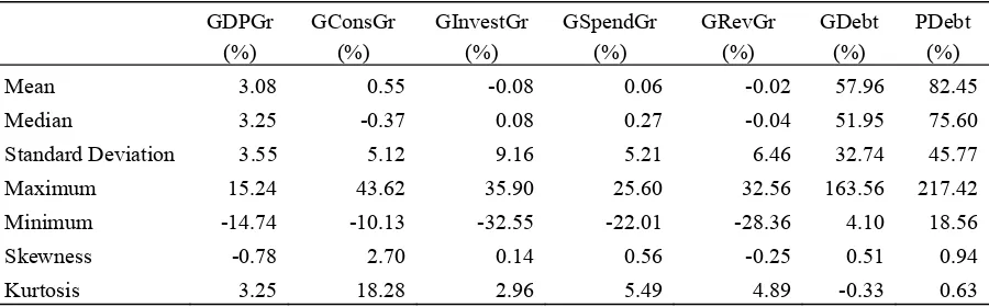
2. Summary Statistics

To provide a data snapshot of those aforementioned variables, the descriptive statis-tics are summarised in table 1 below.

From the table, we point out that the economies tended to implement expansionary fiscal policies during the last two decades by increasing their governments’ expenditures and reducing the tax revenues. Regarding the governments’ spending, the governments are inclined to stimulate their economies through an increase in government consumption. It is clear from the table that the range of debt levels across countries is very wide. This indicates a high variability in the levels of public and private debt among the economies.

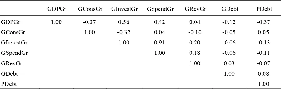
In Table 2, one can see the correlation coefficient among the variables. As can be seen from the table, there is no high correlation among the explanatory variables that might lead to a multicollinearity problem. The exception is between government investment growth and government spending growth, for which the coefficient is close to 100 percent. As explained in the earlier chapter, these two variables will not be used as dependent variables in the same regression model since this research mainly uses the government spending growth as the proxy of spending-based fiscal stimuli.

Table 1 Summary of Descriptive Statistics

GDPGr (%)

GConsGr (%)

GInvestGr (%)

GSpendGr (%)

GRevGr (%)

GDebt (%)

PDebt (%)

Mean 3.08 0.55 -0.08 0.06 -0.02 57.96 82.45

Median 3.25 -0.37 0.08 0.27 -0.04 51.95 75.60

Standard Deviation 3.55 5.12 9.16 5.21 6.46 32.74 45.77

Maximum 15.24 43.62 35.90 25.60 32.56 163.56 217.42

Minimum -14.74 -10.13 -32.55 -22.01 -28.36 4.10 18.56

Skewness -0.78 2.70 0.14 0.56 -0.25 0.51 0.94

Kurtosis 3.25 18.28 2.96 5.49 4.89 -0.33 0.63

(11)

2017 Adi 219 Table 2 Correlation among Variables

GDPGr GConsGr GInvestGr GSpendGr GRevGr GDebt PDebt

GDPGr 1.00 -0.37 0.56 0.42 0.04 -0.12 -0.37

GConsGr 1.00 -0.32 0.04 -0.10 -0.05 0.05

GInvestGr 1.00 0.91 0.20 -0.06 -0.13

GSpendGr 1.00 0.18 -0.06 -0.11

GRevGr 1.00 0.03 -0.07

GDebt 1.00 0.08

PDebt 1.00

Source: The World Bank database; data processed (2015)

RESULTS AND DISCUSSION

1. Spending Multipliers

Four approaches of the panel regression are performed, which are a pooled OLS, a country fixed effect, a time fixed effect, and a country and time fixed effect. The results show that implementing both country and time fixed effects increases the reliability of the regression analysis. Performing the redundant fixed effects tests, the results strongly reject the null hypotheses that the fixed effects are redundant. This means that both fixed effects are necessary and the pooled sample could not be employed (Brooks, 2014). For the next analysis, accordingly, the paper will present merely the regression implementing both the country and time fixed effects.

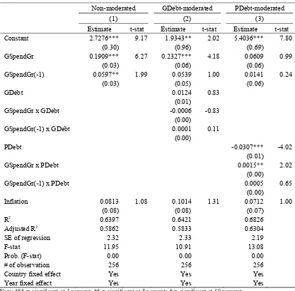
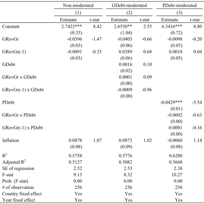
Revisiting the earlier section, one can analyse the moderating effect of public and private debt levels on the spending multiplier using the Equations (2) and (3), consecutively, and comparing them to the basic Equation (1). Table 3 below shows the regression results of those three equations. Having the estimates in column (1), one can see that spending stimulus significantly affects the economy, during both the implementing year and the year after. Moreover, the positive value of the estimates indicates that an increase in government spending leads to a boost in the real GDP. This result is consistent with Keynesians’ arguments. From the table, we can also see that having the interaction variable of the level of public debt does not alter the earlier result. It seems that the

public debt’s level does not moderate the spending multiplier since neither the estimate of “GSpendGr x GDebt” nor “GSpendGr(-1) x GDebt” is statistically different from zero. Controlling for the variable of private debt’s level, on the other hand, one can find different results. In this model, the level of private debt shows a positive moderation effect on the spending stimuli contemporaneously. This means that an increase in the level of private debt might amplify the spending effect on output within the year of implementation.

It is worth noting that the variable of private debt itself appears to behave as an independent variable, since it produces a significant estimate. As it not only interacts with the predictor variable but also is a predictor itself, one might call private debt a quasi-moderator (Sharma, Durand & Gur-Arie, 1981). The significant negative impact of private debt on GDP might cancel out the earlier positive moderating effect on the contemporaneous spending stimuli.

The above regressions provide the estimates of real GDP growth due to the changes in the

governments’ spending growth ( /

(12)

Table 3 Public Spending Effect on Economic Output

Non-moderated GDebt-moderated PDebt-moderated

(1) (2) (3)

Estimate t-stat Estimate t-stat Estimate t-stat Constant 2.7276***

(0.30)

9.17 1.9343** (0.96)

2.02 5.4036*** (0.69)

7.80

GSpendGr 0.1909*** (0.03)

6.27 0.2327*** (0.06)

4.18 0.0609 (0.06)

0.99

GSpendGr(-1) 0.0597** (0.03)

1.99 0.0539 (0.05)

1.00 0.0141 (0.06)

0.24

GDebt 0.0124

(0.01)

0.83

GSpendGr x GDebt -0.0006

(0.00)

-0.83

GSpendGr(-1) x GDebt 0.0001

(0.00)

0.11

PDebt -0.0307***

(0.01)

-4.02

GSpendGr x PDebt 0.0015**

(0.00)

2.02

GSpendGr(-1) x PDebt 0.0005

(0.00)

0.65

Inflation 0.0813 (0.08)

1.08 0.1014 (0.08)

1.31 0.0712 (0.07)

1.00

R2 0.6397 0.6421 0.6826

Adjusted R2 0.5862 0.5833 0.6304

SE of regression 2.32 2.33 2.19

F-stat 11.95 10.91 13.08

Prob. (F-stat) 0.00 0.00 0.00

# of observation 256 256 256

Country fixed effect Yes Yes Yes

Year fixed effect Yes Yes Yes

Note: *** = significant at 1 percent; ** = significant at 5 percent; * = significant at 10 percent; Figures in parentheses refer to standard error of variables

Source: The World Bank database; regression result (2015)

Table 4 Impact and Cumulative Multipliers of Public Spending

(1) (2) (3)

Non-moderated

GDebt-moderated PDebt-moderated

Elasticity 0.1909 0.2003 0.1780

Cumulative elasticity 0.2507 0.1780 0.2285

Total spending to GDP ratio 0.4325 0.4325 0.4325

Impact multiplier 0.4414 0.4613 0.4115

Cumulative multiplier (2yrs) 0.5795 0.5973 0.5283

Note: The elasticity values in column (2) and (3) are calculated by adding the estimate of “GSpendGr” or “GConsGr” or “GInvestGr” with the relevant estimate of the interaction variables (i.e. “GConsGr x GDebt”) multiplied by the median value of the respecting moderator value; whilst the elasticity values in column (1) are simply the estimate of “GSpendGr” or “GConsGr” or “GInvestGr”. The cumulative elasticity is calculated by summing up the elasticity value of the contemporaneous and lagged effect for each component of government expenditure. The ratio on GDP refers to the median value of each component of expenditure to the GDP ratio.

(13)

2017 Adi 221

Without controlling the debt level, the size of the impact multiplier is around 0.44 whilst that of the cumulative multiplier is between 0.58 – 0.59. This result is quite similar to the earlier findings. Blanchard and Perotti (2002) documented the size of the impact multiplier for the first four quarters as being between 0.45 – 0.55 and the cumulative multiplier after eight quarters is between 0.54 – 0.65.

Considering the interaction with public debt, both the impact and cumulative multipliers show a slight increase to 0.46 and 0.60, consecutively. This result does not seem to support the earlier studies, which suggest a negative effect of government debt on the spending multiplier. Regarding the impact of private debt, on the other hand, one can point out a decrease in the spending multipliers. This finding is in line with the work of Cecchetti, Mohanty, and Zampolli (2011) and Jorda, Schularick, and Taylor (2013), which argued that the level of private debt becomes a drag on economic growth. Having this evidence, in addition, the Hypotheses H1 and

H2 do not seem to hold.

As mentioned earlier, this paper also tries to find out the spending effect from the perspective of each of its elements. The analysis follows

Ilzetzki, Mendoza, and Vegh (2013) which put public consumption and investment altogether in one model. The table below exhibits the results for the consumption and investment effects.

As one can see, decomposing government expenditure into its separate elements increases the reliability of the model by more than five percent. The result, moreover, shows that both public consumption and investment significantly affect the economic output. Unlike the positive direction of public expenditure, however, each element has an opposite direction, one to another. Whilst public investment follows the same direction as public expenditure, govern-ment consumption appears to have a negative association with GDP growth. At one point, this finding is in line with Gonzalez-Garcia, Lemus, and Mrkaic (2013) arguing that public investment is more effective in stimulating an economy compared to public consumption. The result also suggests that the economy might view the spending instrument used by the government differently. This advocates the finding of Ilzetzki, Mendoza, and Vegh (2013), arguing that the composition of expenditure may have an important role in determining the impact of the fiscal stimuli, especially in developing countries.

Table 5 Public Consumption and Investment Effects on Economic Output

(1) (2) (3)

(0.27)

10.62 3.1865*** (0.89)

3.58 5.0401*** (0.66)

7.62

GConsGr -0.1123*** (0.03)

-3.55 -0.1685*** (0.05)

-3.47 -0.0719 (0.05)

-1.46

GConsGr(-1) -0.0396 (0.03)

-1.29 -0.0557 (0.05)

-1.20 -0.0192 (0.05)

-0.40

GDebt -0.0057

(0.01)

-0.41

GConsGr x GDebt 0.0015

(0.00)

1.64

GConsGr(-1) x GDebt 0.0005

(0.00)

0.59

PDebt -0.0257***

(0.01)

(14)

GConsGr x PDebt -0.0006 (0.00)

-0.76

GConsGr(-1) x PDebt -0.0002

(0.00)

-0.26

GInvestGr 0.1322*** (0.02)

7.66 0.1605*** (0.03)

5.25 0.1224*** (0.03)

3.50

GInvestGr(-1) 0.0510*** (0.02)

2.99 0.0585** (0.03)

1.95 0.0362 (0.03)

1.06

GInvest x GDebt -0.0004

(0.00)

-1.04

GInvest(-1) x GDebt -0.0002

(0.00)

-0.40

GInvest x PDebt -0.0001

(0.00)

-0.16

GInvest(-1) x PDebt 0.0001

(0.00)

0.14

Inflation 0.0738 (0.07)

1.08 0.0754 (0.07)

1.08 0.0775 (0.07)

1.15

R2 0.7049 0.7149 0.7254

Adjusted R2 0.6580 0.6618 0.6743

F-stat 15.02 13.48 14.20

Prob. (F-stat) 0.00 0.00 0.00

Having the interaction with debt, one cannot observe a moderating effect of both public and private debt on each component of total spending. This result is different from the previous result, which viewed governments’ consumption and investment as total spending. Previously, the contemporaneous moderating effect of private debt appeared to be the case on total public spending. Similar to the earlier analysis, on the other hand, one can still find that the level of private debt has a negative and significant interaction with the dependent variable.

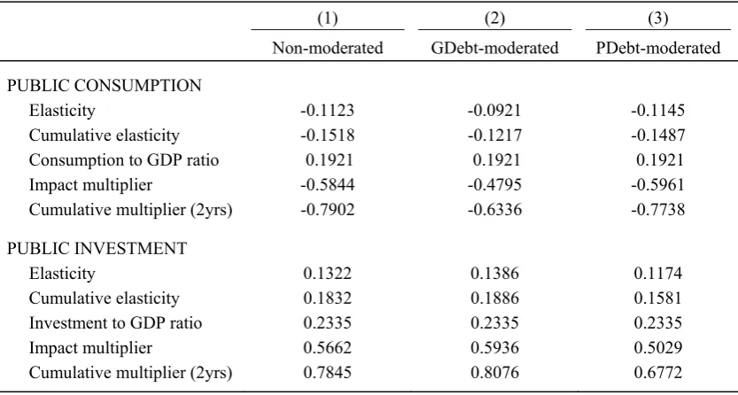
To see how the decomposition of govern-ment expenditure affects the impact and cumulative multipliers, one can see this in Table 6. As one can see, both the impact and

(15)

2017 Adi 223 Table 6 Impact and Cumulative Multipliers of Public Consumption and Investment

(1) (2) (3)

PUBLIC CONSUMPTION

Elasticity -0.1123 -0.0921 -0.1145

Cumulative elasticity -0.1518 -0.1217 -0.1487

Consumption to GDP ratio 0.1921 0.1921 0.1921

Impact multiplier -0.5844 -0.4795 -0.5961

Cumulative multiplier (2yrs) -0.7902 -0.6336 -0.7738

PUBLIC INVESTMENT

Elasticity 0.1322 0.1386 0.1174

Investment to GDP ratio 0.2335 0.2335 0.2335

Note: The elasticity values in column (2) and (3) are calculated by adding the estimate of “GConsGr” or “GInvestGr” with the relevant estimate of the interaction variables (i.e. “GConsGr x GDebt”) multiplied by the median value of the respecting moderator value; whilst the elasticity values in column (1) are simply the estimate of “GConsGr” or “GInvestGr”. The cumulative elasticity is calculated by summing up the elasticity value of the contemporaneous and lagged effect for each component of government expenditure. The ratio on GDP refers to the median value of each component of expenditure to the GDP ratio.

2. Spending Multipliers

Similar to the earlier steps, a series of regressions based on Equations (4), (5) and (6) is run to see the impact of public and private debt levels on the revenue multipliers. Table 7 presents the regression results pertaining to the revenue-based policy’s impact.

As one can see from the table above, there is a negative relationship between government tax revenues and real GDP growth. This means that reducing taxes seems to be an expansionary policy. The result, however, is statistically not different from zero. This evidence advocates the Ricardian equivalence hypothesis’s argument that tax cuts are likely to have no significant impact on the economic output. This is because the current tax cuts are likely to be compensated for with increased taxes in the future (Barsky, Mankiw & Zeldes, 1986).

From the table, we can see no moderating effect of both the public and private debt levels. This can be seen from the estimate of the interaction variables, which are not significantly different from zero. This finding shows that Hypotheses H1 and H2 do not seem to make the case for the revenue multiplier. Similar to the analysis of the impact of spending, one can see that private debt appears to be the explanatory variable of economic output. Like in the analysis of spending’s effects, higher private debt levels are associated with lower GDP growth.

(16)

Table 7 Government Revenue’s Effect on Economic Output

(1) (2) (3)

(0.33)

8.42 2.6530** (1.04)

2.55 6.3416*** (0.72)

8.80

GRevGr -0.0396 (0.03)

-1.47 -0.0403 (0.06)

-0.66 -0.0098 (0.05)

-0.20

GRevGr(-1) -0.0091 (0.03)

-0.33 0.0389 (0.06)

0.68 0.0018 (0.05)

0.04

GDebt 0.0016

(0.02)

0.10

GRevGr x GDebt 0.0001

(0.00)

0.09

GRevGr(-1) x GDebt -0.0009

(0.00)

-0.96

PDebt -0.0429***

(0.01)

-5.54

GRevGr x PDebt -0.0002

(0.00)

-0.63

GRevGr(-1) x PDebt -0.0001

(0.00)

-0.16

Inflation 0.0878 (0.08)

1.07 0.0873 (0.09)

1.02 -0.0060 (0.08)

1.14

R2 0.5758 0.5776 0.6280

Adjusted R2 0.5127 0.5082 0.5668

F-stat 9.13 8.32 10.27

Prob. (F-stat) 0.00 0.00 0.00

Table 8 Impact and Cumulative Multipliers of Government Revenue

(1) (2) (3)

Elasticity -0.0396 -0.0355 -0.0279

Cumulative elasticity -0.0487 -0.0425 -0.0309

Revenue to GDP ratio 0.1877 0.1877 0.1877

Impact multiplier -0.2107 -0.1892 -0.1488

Cumulative multiplier (2yrs) -0.2594 -0.2265 -0.1645

Note: The elasticity values in column (2) and (3) are calculated by adding the estimate of “GRevGr” with the relevant estimate of the interaction variables (i.e. “GRevGr x GDebt”) multiplied by the median value of the respecting moderator value; whilst the elasticity values in column (1) are simply the estimate of “GRevGr”. The cumulative elasticity is calculated by summing up the elasticity value of the contemporaneous and lagged effect for each component of government expenditure. The ratio on GDP refers to the median value of each component of expenditure to the GDP ratio.

(17)

2017 Adi 225

It is obvious from the table that all the multipliers are negative, which means that an increase in the governments’ revenues is apt to reduce the output of the economies. Without considering the interaction with debt, the size of the impact multiplier is around 0.21 – 0.24 whilst that of the cumulative multiplier is between 0.26 – 0.30. In the earlier literature, the revenue multipliers vary widely, ranging from -1.5 to 1.4 (Spilimbergo, Symansky & Schindler, 2009). Our finding is quite close to what Batini, Callegari, and Melina (2012) documented in the case of Japan, which is around -0.3 and -0.2.

Taking the interaction with debt into account, the impact and cumulative multipliers go down with an increase in both the public and private levels of debt. As one can see, private debt seems to make a higher contribution to reducing the multipliers of the revenue’s effect than public debt. From this result, moreover, one can find that private debt consistently reduces the size of the fiscal multipliers for both the spending and revenue stimuli. Public debt, on the other hand, shows a different effect on the multipliers.

As regards the size, one can find that an increase in government spending is likely to generate higher multiplier effects than a tax cut. The former instrument produces impact and cumulative multipliers of around 0.41 – 0.60 whilst the latter accounts for about 0.15 – 0.30. This finding supports the earlier evidence documented by Forni, Monteforte, and Sessa (2009) and Baum, Poplawski-Ribeiro, and Weber (2012), arguing that decreases in taxes are less expansionary than spending increases.

3. Robustness Check

To check whether those results are robust, the same analysis is conducted but with the different set of data, which is the unbalanced panel. As explained earlier, the use of this unbalanced panel enables us to extend the cross-sectional data as well as the time series. In this panel setting, the analysis observes 39 economies from 1991 to 2012. To begin with, the regression results of the spending stimuli

based on an unbalanced panel data set is provided in table 9 below.

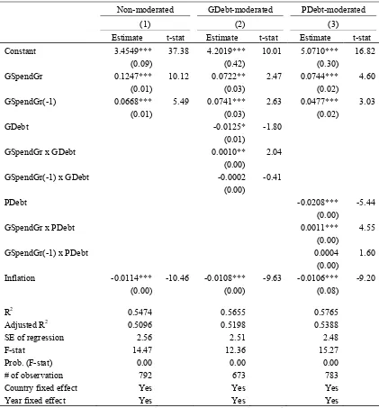
Having the results in Table 9, one can find that the pure effect of the spending stimuli is robust for both types of panel data set; it generates a positive and significant estimate of GDP growth. In addition, utilising the unbalanced panel leads the result to be more statistically significant. Considering the interac-tion with public debt, one can observe a positive moderation effect on the contemporaneous spending effect, as indicated by the positive and significant value of the “GSpendGr x GDebt” coefficient. This finding cannot be found when utilising the balanced panel. Moreover, government debt appears to behave as an explanatory variable of GDP growth. It shows a negative association with the output of the economy at the 10 percent significance level. This result is in line with the literature arguing that the level of public debt should become a drag on the economy.

Regarding the interaction with private debt, one can find similar results with the earlier analysis on the balanced panel. The moderating effect of private debt seems to be the case in both panel settings. In addition, analysing data from the unbalanced panel leads the result to be more statistically significant. The possible explanation as to why one observes results that are more significant is due to the increase in the number of observations. As one can see, the unbalanced panel has twice the data points that the balanced panel has.

(18)

Mrkaic (2013), who found that the effect of government consumption on GDP is statistically not different from zero. This evidence, moreover, emphasises the previous result

arguing that government investment is likely to have a stronger effect in stimulating the economy than government consumption does.

Table 9 Public Spending Effect (Unbalanced Panel)

(1) (2) (3)

(0.09)

37.38 4.2019*** (0.42)

10.01 5.0710*** (0.30)

16.82

GSpendGr 0.1247*** (0.01)

10.12 0.0722** (0.03)

2.47 0.0744*** (0.02)

4.60

GSpendGr(-1) 0.0668*** (0.01)

5.49 0.0741*** (0.03)

2.63 0.0477*** (0.02)

3.03

GDebt -0.0125*

(0.01)

-1.80

GSpendGr x GDebt 0.0010**

(0.00)

2.04

GSpendGr(-1) x GDebt -0.0002

(0.00)

-0.41

PDebt -0.0208***

(0.00)

-5.44

GSpendGr x PDebt 0.0011***

(0.00)

4.55

GSpendGr(-1) x PDebt 0.0004

(0.00)

1.60

Inflation -0.0114*** (0.00)

-10.46 -0.0108*** (0.00)

-9.63 -0.0106*** (0.08)

-9.20

R2 0.5474 0.5655 0.5765

Adjusted R2 0.5096 0.5198 0.5388

F-stat 14.47 12.36 15.27

Prob. (F-stat) 0.00 0.00 0.00

(19)

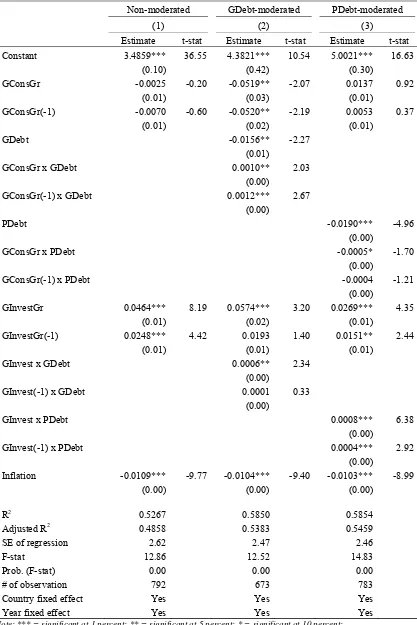
2017 Adi 227 Table 10 Public Consumption and Investment Effect (Unbalanced Panel)

(1) (2) (3)

(0.10)

36.55 4.3821*** (0.42)

10.54 5.0021*** (0.30)

16.63

GConsGr -0.0025 (0.01)

-0.20 -0.0519** (0.03)

-2.07 0.0137 (0.01)

0.92

GConsGr(-1) -0.0070 (0.01)

-0.60 -0.0520** (0.02)

-2.19 0.0053 (0.01)

0.37

GDebt -0.0156**

(0.01)

-2.27

GConsGr x GDebt 0.0010**

(0.00)

2.03

GConsGr(-1) x GDebt 0.0012***

(0.00)

2.67

PDebt -0.0190***

(0.00)

-4.96

GConsGr x PDebt -0.0005*

(0.00)

-1.70

GConsGr(-1) x PDebt -0.0004

(0.00)

-1.21

GInvestGr 0.0464*** (0.01)

8.19 0.0574*** (0.02)

3.20 0.0269*** (0.01)

4.35

GInvestGr(-1) 0.0248*** (0.01)

4.42 0.0193 (0.01)

1.40 0.0151** (0.01)

2.44

GInvest x GDebt 0.0006**

(0.00)

2.34

GInvest(-1) x GDebt 0.0001

(0.00)

0.33

GInvest x PDebt 0.0008***

(0.00)

6.38

GInvest(-1) x PDebt 0.0004***

(0.00)

2.92

Inflation -0.0109*** (0.00)

-9.77 -0.0104*** (0.00)

-9.40 -0.0103*** (0.00)

-8.99

R2 0.5267 0.5850 0.5854

Adjusted R2 0.4858 0.5383 0.5459

F-stat 12.86 12.52 14.83

Prob. (F-stat) 0.00 0.00 0.00

(20)

Having the interaction with the level of debt, one can observe a moderation effect of public debt on both government consumption and investment. This effect cannot be found when the analysis is conducted based on the balanced panel data set. In addition, it is obvious from the table that public debt also negatively interacts with GDP growth. This result is also the case when the analysis is conducted based on total government expenditure.

As regards private debt, one can also observe the moderation effect on government investment as well as government consumption. It seems that private debt has a positive effect on investment stimuli but a negative effect on consumption stimuli. In the balanced panel setting, these effects do not appear to be the case. Moreover, it is noticeable that the moderation effect on public investment is statistically more significant than that on public consumption. In this panel setting, one can also

observe that private debt has a negative and significant estimate on the dependent variable.

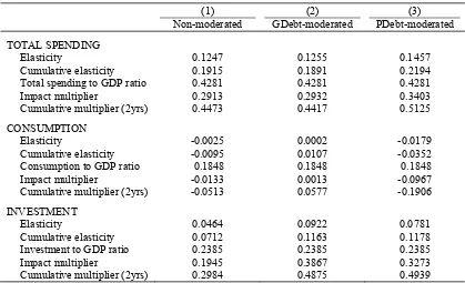
Table 11 provides the size of multipliers based on the unbalanced panel data set. As can be seen from the table, both public and private debts are likely to increase the size of the impact and cumulative multipliers. The biggest impact of public debt on the multipliers is observed in the case of public investment. Private debt, furthermore, shows a similar pattern. Comparing these results with the previous analysis, this finding is quite different from that in the balanced panel data set. In the earlier analysis, spending and investment multipliers are apt to increase with public debt and decrease with private debt. The consumption multiplier, on the other hand, tends to show the opposite pattern to the others.

Next, the robustness check for revenue’s effect on economic output is provided in Table 12 below.

Table 11 Multipliers of Public Spending and Its Components (Unbalanced Panel)

(1) (2) (3)

TOTAL SPENDING

Elasticity 0.1247 0.1255 0.1457

Total spending to GDP ratio 0.4281 0.4281 0.4281

CONSUMPTION

Elasticity -0.0025 0.0002 -0.0179

Cumulative elasticity -0.0095 0.0107 -0.0352

Consumption to GDP ratio 0.1848 0.1848 0.1848

Impact multiplier -0.0133 0.0013 -0.0967

Cumulative multiplier (2yrs) -0.0513 0.0577 -0.1906

INVESTMENT

Elasticity 0.0464 0.0922 0.0781

Investment to GDP ratio 0.2385 0.2385 0.2385

Note: The elasticity values in column (2) and (3) are calculated by adding the estimate of “GSpendGr” or “GConsGr” or “GInvestGr” with the relevant estimate of the interaction variables (i.e. “GConsGr x GDebt”) multiplied by the median value of the respecting moderator value; whilst the elasticity values in column (1) are simply the estimate of “GSpendGr” or “GConsGr” or “GInvestGr”. The cumulative elasticity is calculated by summing up the elasticity value of the contemporaneous and lagged effect for each component of government expenditure. The ratio on GDP refers to the median value of each component of expenditure to the GDP ratio.

(21)

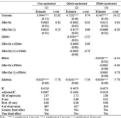
2017 Adi 229 Table 12 Government Revenue Effect (Unbalanced Panel)

(1) (2) (3)

(0.11)

32.02 4.7232*** (0.48)

9.74 6.2437*** (0.43)

14.52

GRevGr 0.0083 (0.01)

0.62 -0.0081 (0.02)

-0.33 0.0151 (0.02)

0.84

GRevGr(-1) 0.0028 (0.01)

0.23 0.0175 (0.03)

0.69 -0.0060 (0.02)

-0.38

GDebt -0.0203**

(0.01)

-2.52

GRevGr x GDebt 0.0003

(0.00)

0.89

GRevGr(-1) x GDebt -0.0003

(0.00)

-0.78

PDebt -0.0339***

(0.01)

-6.34

GRevGr x PDebt -0.0002

(0.00)

-0.88

GRevGr(-1) x PDebt 0.0001

(0.00)

0.78

Inflation -0.0107*** (0.00)

-7.78 -0.0101*** (0.00)

-7.59 -0.0104*** (0.00)

-7.78

R2 0.4519 0.4973 0.4873

Adjusted R2 0.3967 0.4401 0.4320

F-stat 8.18 8.69 8.82

Prob. (F-stat) 0.00 0.00 0.00

From the table, one can see that the governments’ tax revenues generate a positive correlation with real GDP growth. However, the estimates are statistically not different from zero. It means that a revenue-based stimulus is apt to be inconsequential in affecting the economy. Regarding the interaction with the debt level, the result shows that the moderation effect of both public and private debt does not hold for revenue stimuli. This result is also the case in the balanced panel setting. The only different result from the earlier analysis is that one can observe in the unbalanced panel that public debt shows a negative and significant relationship with the dependent variable.

(22)

Table 13 Multipliers of Government Revenue (Unbalanced Panel)

(1) (2) (3)

Elasticity 0.0083 0.0096 0.0055

Revenue to GDP ratio 0.1769 0.1769 0.1769

Note: The elasticity values in column (2) and (3) are calculated by adding the estimate of “GRevGr” with the relevant estimate of the interaction variables (i.e. “GRevGr x GDebt”) multiplied by the median value of the respecting moderator value; whilst the elasticity values in column (1) are simply the estimate of “GRevGr”. The cumulative elasticity is calculated by summing up the elasticity value of the contemporaneous and lagged effect for each component of government expenditure. The ratio on GDP refers to the median value of each component of expenditure to the GDP ratio.

CONCLUSION

Many studies have been conducted to examine the impact of debt on fiscal multipliers. Most of the earlier works, however, focused their analysis merely on public debt. This paper attempts to fill a gap in the literature by taking both public and private debt into account. Unlike Andres, Bosca, and Ferri (2014) who investigated the impact of private debt from the view of household debt in the US economy, this paper provides a broader perspective by employing data of the domestic credit provided to the private sector in several countries. This variable can be expected to cover both corporate and household leverage.

In this paper, fiscal policies are classified into two main categories, which are the spending effect and revenue stimuli. Regarding the pure effect of spending stimuli on economic output, one can observe a positive and significant correlation between government spending and GDP growth. The result is robust for both types of panel setting. This finding advocates the basic Keynesian theory arguing that an increase in government spending will boost the economy.

Furthermore, decomposing public spending into its elements – which are government consumption and investment – one may observe robust evidence that government investment appears to be more effective in stimulating the economy. This finding is in line with that documented by Gonzalez-Garcia, Lemus, and

Mrkaic (2013). Government consumption, on the other hand, surprisingly shows a negative relationship with GDP growth. Nevertheless, this result is not robust. Moreover, this finding suggests that the composition of government expenditure does matter in assessing the effectiveness of fiscal policies.

As regards a revenue-based fiscal policy, one can see an insignificant result for both of the data sets. It indicates that changes in government revenue are likely to have no impact on economic output. This result supports the Ricardian equivalence hypothesis explaining that current tax cuts are merely replaced by higher taxes in the future. Similar findings can be found in the work of Barsky, Mankiw, and Zeldes (1986).

(23)

2017 Adi 231

Regarding private debt’s impact, one might observe a robust moderating effect of private debt on spending stimuli. When the spending stimuli are decomposed into consumption and investment, this effect is not robust and shows a mixed pattern (positive and negative moderation effects) across the two panel data sets. Pertaining to that effect on revenue stimuli, private debt does not show any moderating effect, both in the balanced and unbalanced panel sets. Never-theless, we can find robust evidence that private debt interacts negatively with economic output. This finding is not in line with the work of Andres, Bosca, and Ferri (2014). Conversely, it seems to support the findings of Cecchetti, Mohanty, and Zampolli (2011) and Jorda, Schularik, and Taylor (2013), arguing that over borrowing by the private sector is likely to dampen economic output.

In this paper, two types of multiplier are employed, which are the impact and cumulative multipliers. The table below provides a summary of all the multipliers in several settings. As one can see, the spending impact multiplier has a positive value ranging from 0.29 to 0.44, whilst the cumulative multiplier is between 0.45 and 0.58. The size of the multipliers shows no significant changes when interacting with public debt. Similarly, private debt does not really alter the result. Looking at the spending components, government investment appears to be much more

effective as the expansionary instrument than government consumption. This finding supports the argument that it is crucial to analyse a spending policy’s effectiveness on each of its components separately, since it might produce different results. Regarding the revenue multi-pliers, the impact multiplier is around -0.21 to 0.05 whilst the cumulative multiplier accounts for -0.26 to 0.06. This result remains constant with public debt but decreases slightly when it interacts with private debt.

Finally, one might argue that the use of a panel regression analysis to examine the relationship between fiscal instruments and the output of the economy might be subject to an endogeneity bias. This paper, however, narrows the analysis by focusing on the moderating effect when it is viewed in a one-way causality. To get a more comprehensive perspective of a fiscal policy’s effectiveness, one might utilise the SVAR (Structural Vector Auto Regressions) approach or instrumental variables. Moreover, this paper does not classify the economies into sub samples based on their country-specific characteristics, such as the level of development, exchange rate regime, or openness to trade. Taking that approach into account might be beneficial in providing a more comprehensive result about the impact of public and private debt on a fiscal policy’s effectiveness.

Table 14 Summary of Fiscal Multipliers

(1) (2) (3)

Pure Effect Public Debt Effect Private Debt Effect BALANCED PANEL

Spending 0.44 ; 0.58 0.46 ; 0.60 0.41 ; 0.53

Consumption -0.58 ; -0.79 -0.48 ; -0.63 -0.60 ; -0.77

Investment 0.57 ; 0.78 0.59 ; 0.81 0.50 ; 0.68

Revenue -0.21 ; -0.26 -0.19 ; -0.23 -0.15 ; -0.16

UNBALANCED PANEL

Spending 0.29 ; 0.45 0.29 ; 0.44 0.34 ; 0.51

Consumption -0.01 ; -0.05 0.00 ; 0.06 -0.10 ; -0.19

Investment 0.19 ; 0.30 0.39 ; 0.49 0.33 ; 0.49

Revenue 0.05 ; 0.06 0.05 ; 0.06 0.03 ; 0.04