PIXEL-BASED LAND COVER CLASSIFICATION BY FUSING HYPERSPECTRAL AND
LIDAR DATA
Farah Jahan, Mohammad Awrangjeb
Institute for Integrated and Intelligent Systems, Griffith University, Brisbane, Australia Email: [email protected], [email protected]
KEY WORDS:Hyperspectral, LiDAR, land-cover classification, feature combination, dimensionality reduction
ABSTRACT:
Land cover classification has many applications like forest management, urban planning, land use change identification and environment change analysis. The passive sensing of hyperspectral systems can be effective in describing the phenomenology of the observed area over hundreds of (narrow) spectral bands. On the other hand, the active sensing of LiDAR (Light Detection and Ranging) systems can be exploited for characterising topographical information of the area. As a result, the joint use of hyperspectral and LiDAR data provides a source of complementary information, which can greatly assist in the classification of complex classes. In this study, we fuse hyperspectral and LiDAR data for land cover classification. We do a pixel-wise classification on a disjoint set of training and testing samples for five different classes. We propose a new feature combination by fusing features from both hyperspectral and LiDAR, which achieves competent classification accuracy with low feature dimension, while the existing method requires high dimensional feature vector to achieve similar classification result. Also, for the reduction of the dimension of the feature vector, Principal Component Analysis (PCA) is used as it captures the variance of the samples with a limited number of Principal Components (PCs). We tested our classification method using PCA applied on hyperspectral bands only and combined hyperspectral and LiDAR features. Classification with support vector machine (SVM) and decision tree shows that our feature combination achieves better classification accuracy compared to the existing feature combination, while keeping the similar number of PCs. The experimental results also show that decision tree performs better than SVM and requires less execution time.
1. INTRODUCTION
The use of hyperspectral and Light detection and ranging (Li-DAR) data for land cover classification and tree species classifica-tion has been an active topic of research in recent years (Dalponte et al., 2008; Matsuki et al., 2015; Man et al., 2014; Ghamisi et al., 2015). Hyperspectral sensors capture hundreds of narrow bands of the electromagnetic spectrum from visible to short-wave in-frared wavelengths and provide detailed and continuous spectral information of different objects. On the other hand, LiDAR has been known as a vital method for characterizing vertical struc-tures, including height and volume. As a result, the joint use of hyperspectral and LiDAR data provides a source of complemen-tary information, which can greatly assist in the classification of complex land covers.
Land cover classification methods using the fusion of hyperspec-tral and LiDAR data can be classified into three categories: pixel-level, feature-level and decision level fusion (Priem and Can-ters, 2016; Man et al., 2014). Pixel-level fusion is the lowest level of image fusion which provides original information but is vulnerable to noise and requires relatively long processing time. Feature-level fusion extracts spatial features using object shape and neighbourhood information, spectral and topographical fea-tures by keeping sufficient information with a certain level of ac-curacy. Decision level fusion is the highest level of fusion which combines the classification results in classifier level.
Luo et al. (2016) performed land cover classification using hy-perspectral and LiDAR data and classified seven different classes including buildings, road, water bodies, forests, grassland, crop-land and barren crop-land. They applied pixel based fusion (also called layer stacking) and Principle Component Analysis (PCA) on fused
hyperspectral and LiDAR features. The fusion was done on vary-ing spatial resolutions, which helped to select the best performvary-ing spatial resolution. In this framework, PCA was applied on com-bined hyperspectral and LiDAR features cube ( all features from both modalities applied on a cube), which was different from most of the related work such as Khodadadzadeh et al. (2015) where PCA was used on a single modality (hyperspectral). Man et al. (2015) fused hyperspectral and LiDAR data for urban area classification. Firstly, they used pixel-based fusion and classi-fied land covers separately using support vector machine (SVM) and maximum likelihood (MLC) classifiers. To improve the ac-curacy they combined pixel and object-based classification. In the object-based classification, they set some rules depending on the shape and nature of the classes which were applicable for the dataset that they used but it was not generalised for all the urban areas. Morchhale et al. (2016) investigated classification from the pixel-level fusion of hyperspectral and LiDAR data by ap-plying convolutional neural networks (CNN). Their experimental results proved that pixel-level fusion is an effective approach for the classification using CNN. However, they ignored natural spa-tial relationship among the nearby pixels.
of 2013 IEEE GRSS Data fusion contest introduced a parallel unsupervised and supervised classification. Wang and Glennie (2015) used feature level fusion of synthesised waveform (SWF) and hyperspectral data for land-cover classification. Recently, the fusion of multiple classifiers also improved the classification ac-curacy which is a form of decision level fusion (Bigdeli et al., 2015).
From the above discussion, it is clear that most of the contribu-tions of the previous works were based on pixel-level after ex-tracting spectral and topological features from hyperspectral and LiDAR data. To reduce the misclassification, spatial relationships among the pixels and the shape and volume of the object were also considered after the pixel-based classification as a post clas-sification step. It is a great challenge to select a reduced number of discriminative features from pixel level and selection of appro-priate classifier/classifiers combination which give a generalised model with good performance.
In our method, we undertake pixel-based classification approach using the features extracted from hyperspectral and LiDAR data. Our extracted feature combination is able to classify five different classes with a high classification accuracy with the dimensional-ity of 8. For the classification, we used supervised classifier SVM and decision tree. SVM is the most popular supervised classifier for the classification of hyperspectral and LiDAR data (Dalponte et al., 2008; Luo et al., 2016; Gu et al., 2015; Wang and Glennie, 2015). However, in our case, the decision tree is performing bet-ter than SVM. The main aim of our study is to examine the per-formance of different features from two modalities (hyperspectral and LiDAR) and fuse them in different ways to improve the clas-sification accuracies of various land-cover classes. To accomplish this goal our study contributes in the following ways:
• We implement an image inpainting algorithm for replacing missing LiDAR points for improving the quality of Digital Surface Model (DSM) and intensity images from LiDAR point cloud.
• We compare the performance of our feature combination with the feature combination proposed in (Luo et al., 2016). Our proposed additional features with the features used by Luo et al. (2016) improves the classification accuracies. Ad-ditionally, one of our feature combination without using all hyperspectral bands provides impressive classification accu-racies with limited feature vector dimensionality of 8.
• We implement two fusion techniques named layer stacking and Principal Component Analysis (PCA). We use PCA in two different ways. Firstly, PCA is applied on hyperspectral bands only and additional features with the first few PCs were added. Secondly, PCA is applied on the whole, feature vector from hyperspectral and LiDAR as Luo et al. (2016). Our former technique for using PCA provides higher classi-fication accuracies. Also, we measure the classiclassi-fication ac-curacies of our feature combination and the feature combi-nation proposed by Luo et al. (2016) when applying PCA on the whole feature vector. Our feature combination achieves higher classification accuracies with the same number of PCs than the mentioned existing one using the decision tree.
• Our method for classifying land cover classes is not depen-dent on any prior knowledge like road width/tree height. It can be used in other datasets without any adjustment that is required by some existing method (Man et al., 2015).
• Most of the recent land-cover classification used SVM for classification and SVM outperformed other classifiers. In our case, decision tree outperforms SVM in most of the fea-ture combination with a limited number of feafea-tures. Be-cause our selected features easily categorise samples which fit with the construction structure of the decision tree. As a result, using decision tree we achieve good classification ac-curacies with a limited number of features. Limited number of features reduce the dimension of the feature vector and simplifies the classification process.
• Our methods execute in reasonable CPU processing time. Comparing two supervised classifiers, decision tree outper-forms SVM in terms of execution time. The reason behind faster classification by decision tree is that constructing de-cision tree is computationally inexpensive even when the size of the training set is large.
In this paper section 2 illustrates our proposed methodology where we explain all our approaches in detail. We discuss about registration process, data recovery, feature extraction and mapping in that section. Section 3 discusses our exper-imental setup, brief introduction of input data and experi-mental outcomes. We conclude novelty of our works and future plans in section 4.
2. METHODOLOGY
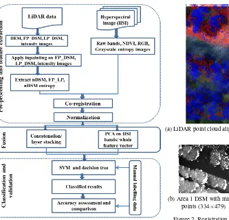
Our framework consists of three main sections including prepro-cessing and feature extraction, fusion and classification, same as other research done on land cover classification. After extract-ing features from both hyperspectral and LiDAR data separately, we fuse them for the classification of five different land cover classes, i.e., “Road”, “Tree”, “Grass”, “Water” and “Soil”. Fig-ure 1 shows the framework of our land-cover classification sys-tem.
2.1 Data Preprocessing
In Figure 1, the first section of preprocessing shows the steps of processing and feature extraction both from hyperspectral and Li-DAR data. It shows two flows of steps coming from LiLi-DAR and hyperspectral that are combined in the co-registration step. In the flow coming from LiDAR, LiDAR point clouds are initially ras-terized according to the pixel size of hyperspectral. In our case, it is 0.5 centimetre. Digital Elevation Model (DEM) is created from the ground return of LiDAR data using ENVI 5.3. The first pulse Digital Surface Model (FP DSM) is generated through rasteriz-ing the first LiDAR return of pixel locations. In the same way, the last pulse Digital Surface Model (LP DSM) is created. We gen-erate the intensity image by calculating the intensity of the first pulse.
Figure 1. Proposed Framework.
functionS characterized by two unknown valuesβ1 andβ2 in Equations (1) and (2):
S(β1, β2)= [10−β1]2+ [β2−β1]2+ [3−β1]2+ [5−β1]2 (1) We will get the unknown valuesβ1andβ2by solving the partial derivative equations of the following:
∂S ∂β1
= 0
∂S ∂β2
= 0
(2)
After co-registration of hyperspectral and LiDAR point cloud, we are able to generate a feature vector for each pixel using fea-tures from both hyperspectral and LiDAR. From Figure 2(a) it is observed that after registration LiDAR point cloud is not properly aligned with the hyperspectral image. From the image, it is clear that LiDAR point cloud is shifted upward in the direction of Y-axis. We manually corrected this registration error for the proper alignment of these two types of data. Figure 2(b) and Figure 2(c) show the DSM with missing LiDAR points (white colours) and the processed DSM after applying inpainting. We normalise the feature vector of each pixel between 0 and 1 as expressed in Equa-tion (3). In EquaEqua-tion (3),x= (x1, x2, . . . , xn)andziis thei
th
normalized data. We do this normalisation because different fea-tures have different ranges of values. But when we fuse them for classification, different ranges of values disrupt the learning and classifying processes of the classifier.
zi=
xi−min(x)
max(x)−min(x) (3)
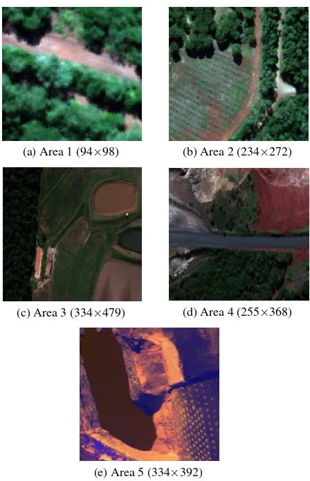
Figure 3 shows the RGB images of five different areas from where
(a) LiDAR point cloud aligned with hyperspectral RGB of Area 1 (94×98)
(b) Area 1 DSM with missing points (334×479)
(c) Area 1 DSM after applying Inpainting
Figure 2. Registration error and inpainting algorithm for recovering missing LiDAR points.
we collected samples for our experiment for the classification of five different land cover classes.
2.2 Feature Extraction
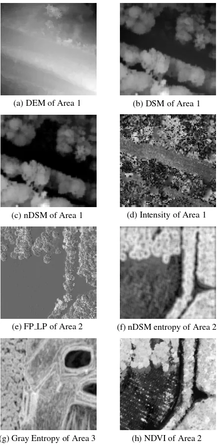
Feature extraction is an important step for land-cover classifica-tion. The classification accuracy depends on the discriminative property of the features extracted from various classes. In this research, we extract spectral and texture features from the hyper-spectral image (HSI). From LiDAR, we extract various height in-formation such as DEM (Digital Elevation Model), DSM (Digital Surface Model), nDSM (Normalised Digital Surface Model), dif-ference between the first and the last LiDAR returns (FP LP), the intensity of the LiDAR pulse and texture information of nDSM like entropy. The following subsection discusses the texture and colour features we use in the land cover classification.
• Normalised Difference Vegetation Index (NDVI)The Nor-malised Difference Vegetation Index (NDVI) is a numerical indicator to evaluate whether the target being observed con-tains live green vegetation Holm AM (1987).
In our case, we calculate NDVI using the following equation
N DV I =RN I R−Rred
RN I R+Rred
(4)
We use NIR (795.16nm, band 42) and Red (679.46nm, band 30) for calculating NDVI using Equation (4). Figure 4(h) shows NDVI image of an area. The tree and grass areas are nearly white for high NDVI. On the other hand, road/soil areas are black for low NDVI.
(DEM) is typically used to represent the height of the bare-earth terrain. Figure 4(a) shows the DEM of Area 1.
• Digital Surface Model (DSM)Digital Surface Model (DSM) captures the height of natural and built features on earth.
In this study, we implement image inpainting techniques for filling missing points values of LiDAR return. Figure 4(b) shows the DSM of Area 1. We discussed our inpainting techniques in the previous section - data preprocessing.
• Normalized Digital Surface Model (nDSM)Normalized Digital Surface Model (nDSM) is calculated by subtracting bare earth returns from the first return reflected by an object on the ground. Figure 4(c) shows the DSM of Area 1.
• Difference Between the First and Last LiDAR Returns (FP LP)In modern LiDAR systems, multiple returns are received for a single laser pulse. In the case of a tree, the laser pulse may go down and partially reflect from different parts of the tree leaves, trunk and branches until it finally hits the bare ground. If there is a solid object like a build-ing or ground, it will just hit the surface. The difference between the first and the last LiDAR returns represents an important property of the reflecting object. We measure the height of first and last LiDAR return of each pixel location
(i, j)and calculate the difference between them. In the case of a tree, the difference is larger than a road/bare surface. Figure 4(e) represents the difference between the first and the last LiDAR returns of a land cover area.
• IntensityLiDAR sensor measures the relative strength of the return pulse which is called intensity. Figure 4(d) shows the intensity image of Area 1. From Figure 4(d) we can observe that the intensity of grass and tree regions varies frequently but the intensity of road is quite stable.
• EntropyIn our land cover classification, entropy gives im-portant texture information for the classification. For ex-ample, the surface of road, tree, grass, water and soil differ from one another in terms of texture smoothness. The sur-face texture of tree and grass are rougher when we compare these to road and water.
Our hyperspectral images contain 62 bands. We select 3 bands associated with red (wavelength 650.84, band 27), green (wavelength 536.64, band 15) and blue (wavelength 564.92, band 18) to generate an RGB image from the hyper-spectral image. The grayscale image is obtained from the RGB image as follows Gonzalez et al. (2003). After con-verting the RGB image into the gray-scale image we calcu-late the entropy of the gray-scale image.
We also calculate entropy from thenDSM(Normalised Dig-ital Surface Model). Trees give higher entropy innDSM
as the surface of the trees frequently varies with height but the road gives lower nDSM entropy. Figure 4(g) represents the gray-level entropy of Area 3 and 4(f) shows the nDSM entropy of the same Area 2. For gray-level entropy, wa-ter represents low entropy value for its smooth texture but grass, tree and soil are contain higher entropy values for their rough texture.
2.3 Data fusion of extracted features
After extracting the features from every pixel, features are con-catenated to produce the signature of each pixel. We produce
(a) Area 1 (94×98) (b) Area 2 (234×272)
(c) Area 3 (334×479) (d) Area 4 (255×368)
(e) Area 5 (334×392)
Figure 3. RGB images and dimensions of five different areas.
nine different types of signatures by combining different features. For fusing data from hyperspectral and LiDAR, we applied two strategies. One is simple layer stacking/ concatenation and an-other is Principal Component Analysis (PCA).
• Concatenation/Layer stackingThis is commonly used method for the fusion of hyperspectral and LiDAR. In layer stack-ing, different features are linearly concatenated to produce the signature of each pixel.
• Principal Component Analysis (PCA)PCA is a useful sta-tistical technique for finding patterns in data of high dimen-sion. PCA transforms the data into a lower dimensional subspace which is optimal in terms of sum-of-squared er-ror (Jolliffe, 2002). PCA reduces the dimensionality of data into a new set of uncorrelated variables, called Principal components (PCs), by a linear transformation of the input data. The first PC has the largest variance (largest eigen-value), the second component has the second largest vari-ance (second largest eigenvalue), etc. PCs are orthogonal to each other and are ordered according to descending eigen-values. We use PCA in two different ways in the fusion technique as discussed before. All the classification results will be shown in the results and discussion section.
2.4 Classification
(a) DEM of Area 1 (b) DSM of Area 1
(c) nDSM of Area 1 (d) Intensity of Area 1
(e) FP LP of Area 2 (f) nDSM entropy of Area 2
(g) Gray Entropy of Area 3 (h) NDVI of Area 2
Figure 4. Eight different features extracted from each area
nature of classification we want to apply. After training, a knowl-edge/model is created by which the machine can categorise un-known samples into several classes based on their attribute val-ues. SVM is the most popular classifier used to classify fused hyperspectral and LiDAR data and in most of the cases, it out-performs Random forests and Maximum likelihood classifiers. For our land cover classification, we use supervised classifiers: Linear SVM and decision tree. The classification accuracies and execution time are reported in the results and discussion section. Decision tree achieved higher classification accuracies than SVM for our dataset and the feature combinations we used for classifi-cation. Also, decision tree classifies data much faster than SVM. The reason behind the smaller execution time of decision tree is that SVM requires parameter tuning to achieve optimal results, while decision tree does not require such tuning process.
3. EXPERIMENTAL RESULT
The data was collected from “Yarraman State Forest” and its adja-cent area located in 170 km north-west of Brisbane, Queensland,
Australia. The total area was almost 8km2. The data was cap-tured 2015 between the month June to July. Table 1 and Table 2 show the sensor parameters which captured LiDAR and hyper-spectral data.
We manually labelled pixels with the help of Google maps. We collected our samples from five different areas shown in Figure 3. Table 3 shows the number of pixels for five different classes. We create 10 different training and testing sets by randomly splitting pixels equally from each class for the evaluation of our methods.
Table 1. LiDAR data
Parameter Specification Recorded returns 6
Average point spacing 0.2m
Table 2. Hyperspectral data
Parameter Specification
Sensor name AISA
Number of Bands 62 (408.54 nm- 990.62 nm) Spatial resolution 0.5 m
Spectral resolution 8.94-9.81 nm
To compare the performance of our features, we develop nine methods by exploring different combinations of the features. We compare the performance of our method with other approaches. We briefly describe our methods as follows:
• Method 1: All 62 bands from hyperspectral data are used for the classification.
• Method 2: Only LiDAR DSM is used for the classification.
• Method 3: All hyperspectral bands and LiDAR DSM, DTM, nDSM and intensity are used for the classification (Luo et al., 2016).
• Method 4: All hyperspectral bands, Gray entropy, NDVI and LiDAR DSM, DTM, nDSM, intensity, FP LP, nDSM entropy are used for the classification.
• Method 5: Gray entropy, NDVI from hyperspectral and Li-DAR DSM, DTM, nDSM, Intensity, FP LP, nDSM entropy are used for the classification.
• Method 6: PCA is used to reduce the dimensionality of HSI data. PCs, LiDAR DSM, DTM, nDSM, Intensity are used for the classification.
• Method 7: PCA is used to reduce the dimensionality of HSI data. PCs, Gray entropy, NDVI, LiDAR DSM, DTM, nDSM, Intensity, FP LP, nDSM entropy are used for the classification.
• Method 8: PCA is applied on the feature vector used in Method 3 (Luo et al., 2016). The PCs are used for the clas-sification.
• Method 9: PCA is applied on the feature vector used in Method 4. The PCs are used for the classification.
Table 3. Distribution of samples collected from five areas for five different classes.
Class Number of Pixels
Road 845
Tree 1422
Grass 821
Water 409
Ground 810
Total 4307
also graphically explain the performance of 9 different methods shows in Figure 5. Method 6 to 9 which use PCA, we consider the accuracies of 5 PCs in Table 5 and Figure 5 but we recorded accu-racies of all PCs. The graphs which shows the accuaccu-racies related to each PCs are shown in Figure 6 and Figure 7. All the methods were programmed in MATLAB on a computer having an Intel Core (TM) i5-4590 processor (3.30 GHz) and 8 GB memory.
Figure 5. Performance of different methods using SVM and decision tree.
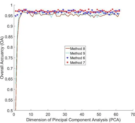
Figure 6. Dimension of PCA and Overall Accuracy (OA) obtained by decision tree.
Figure 7. Dimension of PCA and Overall Accuracy (OA) obtained by SVM.
3.1 Algorithm Evaluation
Accuracy assessment is based on confusion matrix generated by Matlab R2016a. The confusion matrix isn×nmatrix wherenis the number of classes. In the confusion matrix, each row repre-sents the actual class/ground truth and each column reprerepre-sents the predicted class. From the confusion matrix, we calculated overall accuracy (OA) and average accuracy (AA). Before that, we cal-culated precision and class-wise accuracy/recall. The Equations are as follows:
P recision= T rue positive
T rue positive+F alse positive (5)
Accuracy= T rue positive
T rue positive+F alse N egative (6)
OverallAccuracy =
P
Correctly Classif ied Samples T otal N umber of Samples
(7)
AverageAccuracy =
P
Acuuracy of all classes N umber of classes (8)
3.2 Results and Discussion
concate-Table 4. Relationship between features and different methods. ‘Y’ means that a particular feature is used by a method.
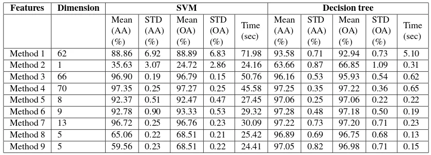
Table 5. Classification accuracies from SVM and decision tree.
Features Dimension SVM Decision tree
Mean
Method 1 62 88.86 6.92 88.89 6.83 71.98 93.58 0.71 92.94 0.73 5.10
Method 2 1 35.63 3.07 24.72 2.86 24.16 63.66 0.87 66.85 1.09 0.31
Method 3 66 96.90 0.19 96.79 0.15 50.76 96.16 0.53 95.93 0.54 0.62
Method 4 70 97.35 0.25 97.27 0.25 45.58 97.25 0.35 97.22 0.36 0.65
Method 5 8 92.37 0.51 92.47 0.47 27.45 97.06 0.25 97.06 0.22 0.22
Method 6 9 92.78 0.90 93.33 0.53 29.32 97.28 0.48 97.18 0.50 0.19
Method 7 13 96.72 0.25 96.76 0.23 30.09 97.22 0.73 97.20 0.71 0.23
Method 8 5 65.06 0.22 68.51 0.21 25.42 96.89 0.69 96.75 0.68 0.13
Method 9 5 59.56 0.23 68.51 0.22 24.41 97.05 0.82 96.98 0.71 0.15
nate them with four LiDAR features DSM, DTM, nDSM and In-tensity. Decision tree AA and OA were 4.5% and 3.85% higher than SVM, respectively. In Method 7, we added additional fea-tures FP LP, nDSM Entropy, Gray Entropy and NDVI with the features of Method 6. The performance of SVM was improved for Method 7 than Method 6. As before, the performance of de-cision tree was a bit higher than SVM for Method 7. Methods 8 and 9 applied PCA on all the features coming from hyperspectral and LiDAR. The feature combination of Method 8 was similar to Method 3 while Method 9 was similar to Method 4. For Method 8 and Method 9, decision tree performed much higher than SVM, approximately 31.83% higher for AA and 28.24% higher for OA.
Method 1 to 5 were based on layer stacking feature fusion from hyperspectral and LiDAR. Among them, Method 4 delivered the highest OA and AA using both SVM and decision tree with a feature vector dimensionality 70. Method 3 represented the fea-ture combination used by (Luo et al., 2016) with dimensionality 66. If we compared the performance of Method 5 and Method 3, Method 5 improved AA by 0.9% and OA by 1.13% using de-cision tree compared to Method 3 while reducing dimensionality from 66 to 8. If we compared the performance of Method 1 and Method 2 with Method 3, Method 4, Method 5, we also noticed that fusing features from hyperspectral and LiDAR improved the classification accuracies as well as reduced the feature vector di-mensionality (Method 5) to a great extent.
Method 6 to Method 9 used PCA for feature fusion from
hyper-spectral and LiDAR. In Method 6 and Method 7 we used PCA to reduce the bands of hyperspectral and add additional features from hyperspectral and LiDAR. Method 8 and Method 9 apply PCA on features from both hyperspectral and LiDAR as exist-ing method (Luo et al., 2016). Method 6 and Method 8 use the feature combination proposed by (Luo et al., 2016). Table 5 and Figure 5 only considered the accuracies of 5 PCs. The graph in Figure 6 and Figure 7 recorded the accuracies of Method 6 to Method 9 considering all PCs. From Table 5 and figures it is clear that Method 6 and Method 7 perform better than Method 8 and Method 9. Keeping the same number of PCs our proposed feature combination Method 7 and Method 9 perform better than Method 6 and Method 8 using both decision tree and SVM.
4. CONCLUSION
(Method 5) with an existing one (Method 3), our proposed fea-ture combination improves OA by 1.13% while reducing feafea-ture dimension from 66 to 8. PCA applied on only HSI bands rather than HSI bands and other LiDAR features prove to be effective for the used dataset. Also, our feature combination (Method 9) achieves higher classification accuracies by using decision tree than the existing feature combination (Method 8) while keep-ing the same number of principal components (5). Decision tree achieves higher classification accuracies than SVM using a lim-ited number of features (reduced feature dimension). On the other hand, SVM achi-eves better accuracies for a large number of fea-tures (Method 3 and 4). Our aim is to achieve good classifica-tion accuracy with a limited number of features that is ignored by other existing studies. Our experimental results proved that deci-sion tree classifier achieves a better result with a limited number of features and also faster than SVM. Our selected feature combi-nation is effective for the discriminative construction of decision tree from the training set, which is also generalised for various land cover classes.
In future, we will try to apply other feature reduction techniques and more advanced spatial feature extraction techniques. Besides this, we are trying to develop a novel feature fusion technique instead of layer stacking method.
REFERENCES
Bigdeli, B., Samadzadegan, F. and Reinartz, P., 2015. Fusion of hyperspectral and LiDAR data using decision template-based fuzzy multiple classifier system. International Journal of Ap-plied Earth Observation and Geoinformation38, pp. 309–320.
Dalponte, M., Bruzzone, L. and Gianelle, D., 2008. Fusion of hy-perspectral and LiDAR remote sensing data for classification of complex forest areas.IEEE Transactions on Geoscience and Remote Sensing46(5), pp. 1416–1427.
Debes, C., Merentitis, A., Heremans, R., Hahn, J., Frangiadakis, N., van Kasteren, T., Liao, W., Bellens, R., Pizurica, A., Gau-tama, S., Philips, W., Prasad, S., Du, Q. and Pacifici, F., 2014. Hyperspectral and LiDAR data fusion: Outcome of the 2013 GRSS data fusion contest. IEEE Journal of Selected Top-ics in Applied Earth Observations and Remote Sensing7(6), pp. 2405–2418.
Ghamisi, P., Benediktsson, J. A. and Phinn, S., 2015. Land-cover classification using both hyperspectral and LiDAR data. Inter-national Journal of Image and Data Fusion6(3), pp. 189–215.
Gonzalez, R. C., Woods, R. E. and Eddins, S. L., 2003. Digital Image Processing Using MATLAB. Prentice-Hall, Inc., Upper Saddle River, NJ, USA.
Gu, Y., Wang, Q., Jia, X. and Benediktsson, J., 2015. A novel MKL model of integrating LiDAR data and MSI for urban area classification. IEEE Transactions on Geoscience and Remote Sensing53(10), pp. 5312–5326.
Holm AM, Burnside DG, M. A., 1987. The development of a sys-tem for monitoring trend in range condition in the arid shrub-lands of western Australia.The Australian Rangeland Journal 9(1), pp. 14–20.
Jolliffe, I., 2002. Principal Component Analysis. Wiley Online Library.
Khodadadzadeh, M., Li, J., Prasad, S. and Plaza, A., 2015. Fusion of hyperspectral and LiDAR remote sensing data using multi-ple feature learning. IEEE Journal of Selected Topics in Ap-plied Earth Observations and Remote Sensing8(6), pp. 2971– 2983.
Luo, S., Wang, C., Xi, X., Zeng, H., Li, D., Xia, S. and Wang, P., 2016. Fusion of airborne discrete-return LiDAR and hy-perspectral data for land cover classification. Remote Sensing 8(1), pp. 3–22.
Man, Q., Dong, P. and Guo, H., 2015. Pixel- and feature-level fusion of hyperspectral and LiDAR data for urban land-use classification.International Journal of Remote Sensing36(6), pp. 1618–1644.
Man, Q., Dong, P., Guo, H., Liu, G. and Shi, R., 2014. Light detection and ranging and hyperspectral data for estimation of forest biomass: a review. Journal of Applied Remote Sensing 8(1), pp. 081598–1–081598–21.
Matsuki, T., Yokoya, N. and Iwasaki, A., 2015. Hyperspectral tree species classification of Japanese complex mixed forest with the aid of LiDAR data. IEEE Journal of Selected Top-ics in Applied Earth Observations and Remote Sensing8(5), pp. 2177–2187.
Morchhale, S., Pauca, V. P., Plemmons, R. J. and Torgersen, T. C., 2016. Classification of pixel-level fused hyperspectral and LiDAR data using deep convolutional neural networks. In: 8th Workshop on Hyperspectral Image and Signal Processing: Evolution in Remote Sensing (WHI.SPERS), Los Angeles, CA.
Pingel, T. J., Clarke, K. C. and McBride, W. A., 2013. An im-proved simple morphological filter for the terrain classification of airborne LiDAR data. ISPRS Journal of Photogrammetry and Remote Sensing77, pp. 21 – 30.
Priem, F. and Canters, F., 2016. Synergistic use of LiDAR and APEX hyperspectral data for high-resolution urban land cover mapping.Remote Sensing8(10), pp. 787–809.