COMMUNICATIONS
Registered Office
John Wiley & Sons Ltd, The Atrium, Southern Gate, Chichester, West Sussex, PO19 8SQ, United Kingdom
For details of our global editorial offices, for customer services and for information about how to apply for permission to reuse the copyright material in this book please see our website at www.wiley.com.
The right of the author to be identified as the author of this work has been asserted in accordance with the Copyright, Designs and Patents Act 1988.
All rights reserved. No part of this publication may be reproduced, stored in a retrieval system, or transmitted, in any form or by any means, electronic, mechanical, photocopying, recording or otherwise, except as permitted by the UK Copyright, Designs and Patents Act 1988, without the prior permission of the publisher.
Wiley also publishes its books in a variety of electronic formats. Some content that appears in print may not be available in electronic books.
Designations used by companies to distinguish their products are often claimed as trademarks. All brand names and product names used in this book are trade names, service marks, trademarks or registered trademarks of their respective owners. The publisher is not associated with any product or vendor mentioned in this book.
Limit of Liability/Disclaimer of Warranty: While the publisher and author have used their best efforts in preparing this book, they make no representations or warranties with respect to the accuracy or completeness of the contents of this book and specifically disclaim any implied warranties of merchantability or fitness for a particular purpose. It is sold on the understanding that the publisher is not engaged in rendering professional services and neither the publisher nor the author shall be liable for damages arising herefrom. If professional advice or other expert assistance is required, the services of a competent professional should be sought
Library of Congress Cataloging-in-Publication Data
Names:Şafak, Mehmet, 1948–author.
Title: Digital communications / MehmetŞafak.
Description: Chichester, UK ; Hoboken, NJ : John Wiley & Sons, 2017. | Includes bibliographical references and index.
Identifiers: LCCN 2016032956 (print) | LCCN 2016046780 (ebook) | ISBN 9781119091257 (cloth) | ISBN 9781119091264 (pdf) | ISBN 9781119091271 (epub)
Subjects: LCSH: Digital communications.
Classification: LCC TK5103.7 .S24 2017 (print) | LCC TK5103.7 (ebook) | DDC 621.382–dc23
LC record available at https://lccn.loc.gov/2016032956
A catalogue record for this book is available from the British Library. Cover Design: Wiley
Cover Image: KTSDESIGN/Gettyimages
Set in 10 /12pt Times by SPi Global, Pondicherry, India
Preface xiv
List of Abbreviations xviii
About the Companion Website xxi
1 Signal Analysis 1
1.1 Relationship Between Time and Frequency Characteristics of Signals 2
1.1.1 Fourier Series 2
1.1.2 Fourier Transform 4
1.1.3 Fourier Transform of Periodic Functions 13
1.2 Power Spectal Density (PSD) and Energy Spectral Density (ESD) 15
1.2.1 Energy Signals Versus Power Signals 15
1.2.2 Autocorrelation Function and Spectral Density 16
1.3 Random Signals 18
1.3.1 Random Variables 18
1.3.2 Random Processes 20
1.4 Signal Transmission Through Linear Systems 27
References 31
Problems 31
2 Antennas 33
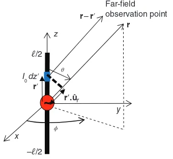
2.1 Hertz Dipole 34
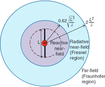
2.1.1 Near- and Far-Field Regions 37
2.2 Linear Dipole Antenna 40
2.3 Aperture Antennas 43
2.4 Isotropic and Omnidirectional Antennas 47
2.5 Antenna Parameters 48
2.5.1 Polarization 48
2.5.2 Radiation Pattern 51
2.5.3 Directivity and Beamwidth 53
2.5.5 Effective Receiving Area 61 2.5.6 Effective Antenna Height and Polarization Matching 68
2.5.7 Impedance Matching 70
References 78
Problems 78
3 Channel Modeling 82
3.1 Wave Propagation in Low- and Medium-Frequency Bands (Surface Waves) 83
3.2 Wave Propagation in the HF Band (Sky Waves) 84
3.3 Wave Propagation in VHF and UHF Bands 85
3.3.1 Free-Space Propagation 86
3.3.2 Line-Of-Sight (LOS) Propagation 86
3.3.3 Fresnel Zones 87
3.3.4 Knife-Edge Diffraction 90
3.3.5 Propagation Over the Earth Surface 95
3.4 Wave Propagation in SHF and EHF Bands 106
3.4.1 Atmospheric Absorption Losses 108
3.4.2 Rain Attenuation 110
3.5 Tropospheric Refraction 118
3.5.1 Ducting 121
3.5.2 Radio Horizon 123
3.6 Outdoor Path-Loss Models 123
3.6.1 Hata Model 124
3.6.2 COST 231 Extension to Hata Model 125
3.6.3 Erceg Model 128
3.7 Indoor Propagation Models 129
3.7.1 Site-General Indoor Path Loss Models 130
3.7.2 Signal Penetration Into Buildings 132
3.8 Propagation in Vegetation 134
References 137
Problems 137
4 Receiver System Noise 145
4.1 Thermal Noise 146
4.2 Equivalent Noise Temperature 147
4.2.1 Equivalent Noise Temperature of Cascaded Subsystems 149
4.3 Noise Figure 150
4.3.1 Noise Figure of a Lossy Device 152
4.4 External Noise and Antenna Noise Temperature 153
4.4.1 Point Noise Sources 154
4.4.2 Extended Noise Sources and Brightness Temperature 154
4.4.3 Antenna Noise Figure 156
4.4.4 Effects of Lossy Propagation Medium on the Observed Brightness
Temperature 156
4.4.5 Brightness Temperature of Some Extended Noise Sources 160
4.4.6 Man-Made Noise 167
4.6 Additive White Gaussian Noise Channel 174
References 175
Problems 175
5 Pulse Modulation 184
5.1 Analog-to-Digital Conversion 185
5.1.1 Sampling 186
5.1.2 Quantization 193
5.1.3 Encoding 203
5.1.4 Pulse Modulation Schemes 204
5.2 Time-Division Multiplexing 209
5.2.1 Time Division Multiplexing 209
5.2.2 TDM Hierarchies 210
5.2.3 Statistical Time-Division Multiplexing 212
5.3 Pulse-Code Modulation (PCM) Systems 212
5.3.1 PCM Transmitter 213
5.3.2 Regenerative Repeater 213
5.3.3 PCM Receiver 214
5.4 Differential Quantization Techniques 220
5.4.1 Fundamentals of Differential Quantization 220
5.4.2 Linear Prediction 221
5.4.3 Differential PCM (DPCM) 226
5.4.4 Delta Modulation 228
5.4.5 Audio Coding 232
5.4.6 Video Coding 234
References 236
Problems 236
6 Baseband Transmission 245
6.1 The Channel 245
6.1.1 Additive White Gaussian Noise (AWGN) Channel 248
6.2 Matched Filter 249
6.2.1 Matched Filter Versus Correlation Receiver 252
6.2.2 Error Probability For Matched-Filtering in AWGN Channel 255
6.3 Baseband M-ary PAM Transmission 263
6.4 Intersymbol Interference 268
6.4.1 Optimum Transmit and Receive Filters in an Equalized Channel 270 6.5 Nyquist Criterion for Distortionless Baseband Binary Transmission In a
ISI Channel 272
6.5.1 Ideal Nyquist Filter 273
6.5.2 Raised-Cosine Filter 276
6.6 Correlative-Level Coding (Partial-Response Signalling) 278
6.6.1 Probability of Error in Duobinary Signaling 280
6.6.2 Generalized Form of Partial Response Signaling (PRS) 282
6.7 Equalization in Digital Transmission Systems 283
References 287
7 Optimum Receiver in AWGN Channel 298
7.1 Introduction 298
7.2 Geometric Representation of Signals 300
7.3 Coherent Demodulation in AWGN Channels 302
7.3.1 Coherent Detection of Signals in AWGN Channels 305
7.4 Probability of Error 311
7.4.1 Union Bound on Error Probability 313
7.4.2 Bit Error Versus Symbol Error 316
References 319
Problems 319
8 Passband Modulation Techniques 323
8.1 PSD of Passband Signals 324
8.1.1 Bandwidth 325
8.1.2 Bandwidth Efficiency 326
8.2 Synchronization 327
8.2.1 Time and Frequency Standards 330
8.3 Coherently Detected Passband Modulations 332
8.3.1 Amplitude Shift Keying (ASK) 333
8.3.2 Phase Shift Keying (PSK) 338
8.3.3 Quadrature Amplitude Modulation (QAM) 352
8.3.4 Coherent Orthogonal Frequency Shift Keying (FSK) 358
8.4 Noncoherently Detected Passband Modulations 367
8.4.1 Differential Phase Shift Keying (DPSK) 367
8.4.2 Noncoherent Orthogonal Frequency Shift Keying (FSK) 370
8.5 Comparison of Modulation Techniques 374
References 378
Problems 379
9 Error Control Coding 386
9.1 Introduction to Channel Coding 386
9.2 Maximum Likelihood Decoding (MLD) with Hard and Soft Decisions 390
9.3 Linear Block Codes 396
9.3.1 Generator and Parity Check Matrices 398
9.3.2 Error Detection and Correction Capability of a Block Code 402
9.3.3 Syndrome Decoding of Linear Block Codes 405
9.3.4 Bit Error Probability of Block Codes with Hard-Decision Decoding 408 9.3.5 Bit Error Probability of Block Codes with Soft-Decision Decoding 409
9.3.6 Channel Coding Theorem 411
9.3.7 Hamming Codes 412
9.4 Cyclic Codes 415
9.4.1 Generator Polynomial and Encoding of Cyclic Codes 415
9.4.2 Parity-Check Polynomial 418
9.4.3 Syndrome Decoding of Cyclic Codes 419
9.4.4 Cyclic Block Codes 422
9.5 Burst Error Correction 429
9.5.2 Reed-Solomon (RS) Codes 432
9.5.3 Low-Density Parity Check (LDPC) Codes 435
9.6 Convolutional Coding 436
9.6.1 A Rate-½ Convolutional Encoder 437
9.6.2 Impulse Response Representation of Convolutional Codes 438 9.6.3 Generator Polynomial Representation of Convolutional Codes 438 9.6.4 State and Trellis Diagram Representation of a Convolutional Codes 439
9.6.5 Decoding of Convolutional Codes 441
9.6.6 Transfer Function and Free Distance 445
9.6.7 Error Probability of Convolutional Codes 447
9.6.8 Coding Gain of Convolutional Codes 451
9.7 Concatenated Coding 454
9.8 Turbo Codes 456
9.9 Automatic Repeat-Request (ARQ) 459
9.9.1 Undetected Error Probability 461
9.9.2 Basic ARQ Protocols 463
9.9.3 Hybrid ARQ Protocols 467
Appendix 9A Shannon Limit For Hard-Decision and Soft-Decision Decoding 471
References 473
Problems 473
10 Broadband Transmission Techniques 479
10.1 Spread Spectrum 481
10.1.1 PN Sequences 481
10.1.2 Direct Sequence Spread Spectrum 485
10.1.3 Frequency Hopping Spread Spectrum 508
10.2 Orthogonal Frequency Division Multiplexing (OFDM) 519
10.2.1 OFDM Transmitter 520
10.2.2 OFDM Receiver 523
10.2.3 Intercarrier Interference (ICI) in OFDM Systems 529
10.2.4 Channel Estimation by Pilot Subcarriers 531
10.2.5 Synchronization of OFDM Systems 532
10.2.6 Peak-to-Average Power Ratio (PAPR) in OFDM 532
10.2.7 Multiple Access in OFDM Systems 539
10.2.8 Vulnerability of OFDM Systems to Impulsive Channel 543
10.2.9 Adaptive Modulation and Coding in OFDM 544
Appendix 10A Frequency Domain Analysis of DSSS Signals 545
Appendix 10B Time Domain Analysis of DSSS Signals 547
Appendix 10C SIR in OFDM systems 548
References 551
Problems 552
11 Fading Channels 557
11.1 Introduction 558
11.2 Characterisation of Multipath Fading Channels 559
11.2.1 Delay Spread 562
11.2.2 Doppler Spread 569
11.3 Modeling Fading and Shadowing 582
11.3.1 Rayleigh Fading 582
11.3.2 Rician Fading 584
11.3.3 Nakagami-m Fading 587
11.3.4 Log-Normal Shadowing 591
11.3.5 Composite Fading and Shadowing 596
11.3.6 Fade Statistics 600
11.4 Bit Error Probability in Frequency-Nonselective Slowly Fading Channels 604
11.4.1 Bit Error Probability for Binary Signaling 605
11.4.2 Moment Generating Function 607
11.4.3 Bit Error Probability for M-ary Signalling 610
11.4.4 Bit Error Probability in Composite Fading and Shadowing Channels 613
11.5 Frequency-Selective Slowly-Fading Channels 614
11.5.1 Tapped Delay-Line Channel Model 615
11.5.2 Rake Receiver 617
11.6 Resource Allocation in Fading Channels 622
11.6.1 Adaptive Coding and Modulation 622
11.6.2 Scheduling and Multi-User Diversity 623
References 626
Problems 626
12 Diversity and Combining Techniques 638
12.1 Antenna Arrays in Non-Fading Channels 640
12.1.1 SNR 647
12.2 Antenna Arrays in Fading Channels 650
12.3 Correlation Effects in Fading Channels 654
12.4 Diversity Order, Diversity Gain and Array Gain 657
12.4.1 Tradeoff Between the Maximum Eigenvalue and the Diversity Gain 659
12.5 Ergodic and Outage Capacity in Fading Channels 660
12.5.1 Multiplexing Gain 663
12.6 Diversity and Combining 664
12.6.1 Combining Techniques for SIMO Systems 666
12.6.2 Transmit Diversity (MISO) 686
References 691
Problems 692
13 MIMO Systems 701
13.1 Channel Classification 702
13.2 MIMO Channels with Arbitrary Number of Transmit and Receive Antennas 703
13.3 Eigenvalues of the Random Wishart Matrix HHH 707
13.3.1 Uncorrelated Central Wishart Distribution 708
13.3.2 Correlated Central Wishart Distribution 710
13.4 A 2 × 2 MIMO Channel 718
13.5 Diversity Order of a MIMO System 722
13.6 Capacity of a MIMO System 723
13.6.1 Water-Filling Algorithm 728
13.7.1 Bit Error Probability in MIMO Beamforming Systems 732
13.8 Transmit Antenna Selection (TAS) in MIMO Systems 734
13.9 Parasitic MIMO Systems 740
13.9.1 Formulation 741
13.9.2 Output SNR 743
13.9.3 Radiation Pattern 744
13.9.4 Bit Error Probability 744
13.9.5 5 × 5 Parasitic MIMO-MRC 746
13.10 MIMO Systems with Polarization Diversity 748
13.10.1 The Channel Model 748
13.10.2 Spatial Multiplexing (SM) with Polarization Diversity 750 13.10.3 MIMO Beamforming-MRC System with Polarization Diversity 751
13.10.4 Simulation Results 751
References 753
Problems 755
14 Cooperative Communications 758
14.1 Dual-Hop Amplify-and-Forward Relaying 759
14.1.1 Source-Relay-Destination Link with a Single Relay 760
14.1.2 Combined SRD and Direct Links 765
14.2 Relay Selection in Dual-Hop Relaying 767
14.2.1 Relay Selection Strategies 769
14.2.2 Performance Evaluation of Selection-Combined Best SRD
and SD Links 769
14.3 Source and Destination with Multiple Antennas in Dual-Hop AF Relaying 776
14.3.1 Source-Relay-Destination Link 776
14.3.2 Source-Destination Link 782
14.3.3 Selection-Combined SRD and SD Links 783
14.4 Dual-Hop Detect-and-Forward Relaying 787
14.5 Relaying with Multiple Antennas at Source, Relay and Destination 796
14.6 Coded Cooperation 798
Appendix 14A CDF ofγeqandγeq,0 800
Appendix 14B Average Capacity ofγeq,0 801
Appendix 14C Rayleigh Approximation for Equivalent SNR with Relay Selection 802
Appendix 14D CDF ofγeq,a 804
References 806
Problems 807
Appendix A: Vector Calculus in Spherical Coordinates 810
Appendix B: Gaussian Q Function 811
Appendix C: Fourier Transforms 819
Appendix D: Mathematical Tools 821
Appendix E: The Wishart Distribution 834
Appendix F: Probability and Random Variables 844
Telecommunications is a rapidly evolving area of electrical engineering, encompassing diverse areas of applications, including RF communi-cations, radar systems, ad-hoc networks, sensor networks, optical communications, radioastr-onomy, and so on. Therefore, a solid back-ground is needed on numerous topics of electrical engineering, including calculus, antennas, wave propagation, signals and sys-tems, random variables and stochastic pro-cesses and digital signal processing. In view of the above, the success in the telecommunica-tions education depends on the background of the student in these topics and how these topics are covered in the curriculum. For example, the Fourier transform may not usually be taught in relation with time- and frequency-response of the systems. Similarly, concepts of probabiliy may not be related to random signals. On the other hand, students studying telecommunica-tions may not be expected to know the details of the Maxwell’s equations and wave propaga-tion. However, in view of the fact that wireless communication systems comprise transmit/ receive antennas and a propagation medium, it is necessary to have a clear understanding of the radiation by the transmit antenna, propa-gation of electromagnetic waves in the con-sidered channel and the reception of
electromagnetic waves by the receive antenna. Otherwise, the students may face difficulties in understanding the telecommunications process in the physical layer.
The engineering education requires a careful tradeoff between the rigour provided by the the-ory and the simple exposure of the correspond-ing physical phenomena and their applications in our daily life. Therefore, the book aims to help the students to understand the basic principles and to apply them. Basic principles and analyt-ical tools are provided for the design of commu-nication systems, illustrated with examples, and supported by graphical illustrations.
illustrations, figures, examples, references, and problems for better understanding the exposed concepts.
Chapter 1 Signal Analysis summarizes the time-frequency relationship and basic concepts of Fourier transform for deterministic and ran-dom signals used in the linear systems. The aim was to provide a handy reference and to avoid repeating the same basic concepts in the subsequent chapters.Chapter 2 Antennas pre-sents the fundamentals of the antenna theory with emphasis on the telecommunication aspects rather than on the Maxwell’s equations.Chapter 3 Channel Modelingpresents the propagation pro-cesses following the conversion of the electrical signals in the transmitter into electromagnetic waves by the transmit antenna until they are reconverted into electrical signals by the receive antenna.Chapter 4 System Noiseis mainly based on the standards for determining the receiver noise of internal and external origin and provides tools for calculating SNR at the receiver output; the SNR is known to be the figure-of-merit of communication systems since it determines the system performance. Chapters 2, 3 and 4 thus relate the wireless interaction between transmit-ter and receiver in the physical layer. It may be worth mentioning that, unlike many books on wireless communications, covering only VHF and UHF bands, Chapters 2, 3 and 4 extend the coverage of antennas, receiver noise and channel modeling to SHF and EHF bands. A thorough understanding of the materials pro-vided in these chapters is believed to be critical for deeper understanding of the rest of the book. These three chapters are believed to close the gap between the approaches usually followed by books on antennas and RF propagation, based on the Maxwell’s equations, and the books on digital communications, based on statistical the-ory of communications. One of the aims of the book is to help the students to fuse these two complementary approaches.
The following chapters are dedicated to stat-istical theory of digital communications. Chap-ter 4 Pulse Modulation treats the conversion of analog signals into digital for digital
potential sources of interference. Source coding is not addressed in the book. Channel coding usually comes at the expense of increased trans-mission rate, hence wider transtrans-mission band-width, due to the inclusion of additional (parity check) bits among the data bits. Use of parity check bits reduces energy per channel bits and hence leads to higher channel BEP. However, a good code is expected to correct more errors than it creates and the overall coded BEP decreases at the expense of increased transmis-sion bandwidth. This tradeoff between the BEP and the transmission bandwidth is well-known in the coding theory. As shown by the Shannon capacity theorem, one can achieve error-free communications as the transmission bandwidth goes to infinity, that is, by using infin-itely many parity check bits, as long as the ratio of the energy per bit to noise PSD (Eb/N0) is higher than −1.6 dB. This chapter addresses block and convolutional codes which are capable of correcting random and burst-errors. Auto-matic-repeat request (ARQ) techniques based on error-detection codes and hybrid ARQ (HARQ) techniques exploiting codes which can both detect and correct channel bit errors are also presented. Chapter 10 Broadband Transmission Techniquesis composed of mainly two sections, namely spread-spectrum (SS) and the orthogonal frequency division multiplexing (OFDM). SS and OFDM provide alternative approaches for transmission of multi-user sig-nals over wide transmission bandwidths. In SS, spread multi-user signals are distinguished from each other by orthogonal codes, while, in OFDM, narrowband multi-user signals are trans-mitted with different orthogonal subcarriers. The chapter is focused on two versions of SS, namely the direct sequence (DS) SS and frequency-hopping (FH) SS. Intercarrier- and intersym-bol-interference, channel estimation and syn-chronization, adaptive modulation and coding, peak-to-average power ratio, and multiple access in up- and down-links of OFDM systems are also presented. Chapter 11 Fading Channels accounts for the effects of multipath propagation and shadowing. Fading channels are usually
an NtNr-fold antenna diversity (NtNr inde-pendent paths between transmitter and receiver). The MIMO channels is usually char-acterized by Wishart distribution, presented in Appendix E. The eigenvalues of random Wishart matrices determine the dominant characteristics of the MIMO channels, which may suffer correlation between the transmitted and/or received signals. This determines the number and the relative weights of the eigen-modes; water-filling algorithm can be used to equalize the transmit power or the data rate supported by each eignmode. Transmit antenna selection (TAS) implies the selection of one or a few of the multiple transmit anten-nas with highest instantaneous SNRs. TAS makes good use of the transmit diversity by dividing the transmit power only between the transmit antennas with highest instantan-eous SNRs. MIMO systems enjoy full coord-ination between transmit and receive antennas. Consequently, by adjusting the complex antenna weights at the transmit- and receive-sides, the SNR at the output of a MIMO beam-forming system can be maximized, hence min-imizing the BEP. Chapter 14 on Cooperative Communicationsis based on dual-hop relaying with amplify-and-forward, detect-and-forward and coded cooperation protocols. The source-relay-destination link is modeled as a single link with an equivalent SNR, the relay with the high-est equivalent SNR may be selected amongst a number of relays, and multiple antennas may be used at the source, at the relay and/or the des-tination. The source-destination link is usually selection- or maximal-ratio-combined with the source-relay-destination link. In coded cooper-ation, relaying and channel coding are simul-taneously used to make better use of the cooperation.
The appendices are believed to provide con-venient references, and useful background for
better understanding of the relevant concepts. Appendix A Vector Calculus in Spherical Coord-inates provides tools for conversion between spherical and polar coordinates required for Chapter 2 Antennas. Appendix B Gaussian Q Functionis useful for determining the BEP of majority of modulation schemes. Appendix Cpresents a list of Fourier Transforms usually encountered in telecommunication applications. Appendix D Mathematical Toolspresents series, integrals and functions used in the book, minim-izing the need to resort to another mathematical handbook. Appendix E Wishart Distribution provides the necessary background for the Chapter 13 MIMO Systems.Appendix F Prob-ability and Random Variablesaims to help stu-dents with probabilistic concepts, widely used probability distributions and random processes. Topics to be taught at undergraduate and graduate levels may be decided according to the priority of the instructor and the course con-tents. Some sections and/or chapters may be omitted or covered partially depending on the preferences of the instructor. However, it may not be easy to give a unique approach for spe-cifying the curriculum.
During my career, I benefited from numer-ous excellent books, publications and Internet web pages. I would like to thank the authors of all sources who contributed for the accumu-lation of the knowledge reflected in this book. I would like to thank all my undergraduate and graduate students who, with their response to my teaching approaches, helped enormously for determining the contents and the coverage of the topics of this book. Valuable cooperation and help from Sandra Grayson, Preethi Belkese and Adalfin Jayasingh from John Wiley and Sons is highly appreciated.
ACK acknowledgment
ADC analog-to-digital conversion
ADM adaptive delta modulation
AF amplify and forward
AGC automatic gain control
AJ anti jamming
AMR adaptive multi rate
AOA angle of arrival
AOD angle of departure
AOF amount of fading
ARQ automatic repeat request
ASK amplitude shift keying
AT&T American Telephone & Telegraph Company
AWGN additive white Gaussian noise
BCH Bose-Chaudhuri-Hocquenghem
codes
BEP bit error probability BPSK binary phase shift keying
BS base station
BSC binary symmetric channel
C/N carrier-to-noise ratio CCITT International Telegraph and
Telephone Consultative Committee
CD compact disc
CDF cumulative distribution function CDMA code division multiple access
CIR channel impulse response
COST European Cooperation for
Scientific and Technical Research
CP cyclic prefix
CPA co-polar attenuation
CRC cyclic redundancy check
CSI channel state information DAC digital to analog conversion DCT discrete cosine transform
DF detect and forward
DFT discrete Fourier transform
DGPS differential GPS
DM delta modulation
DMC discrete memoryless channel
DPCM differential PCM
DPSK differential phase shift keying
DS direct sequence
DSSS direct sequence spread spectrum
E1 European telephone
multiplex-ing hierarchy
EGC equal gain combining
EGNOS European geostationary navigation overlay service EHF extremely high frequencies
(30-300 GHz)
EIRP effective isotropic radiative power
EP elliptical polarization
ETSI European Telecommunications Standards Institute
FDM frequency division multiplexing FEC forward error correction FFT fast Fourier transform
FH frequency hopping
FHSS frequency hopping spread
spectrum
FIR finite impulse response
FOM figure of merit
FSK frequency shift keying
FT Fourier transform
G/T figure of merit of a receiver (antenna gain to system noise temperature ratio)
GALILEO European global navigation satellite system
GBN go-back-N ARQ
GEO geostationary
GLONASS Russian global navigation satellite system
GNSS global navigation satellite systems
GPS global positioning system
GS greedy scheduling
GSC generalized selection combining
GSM global system for mobile
communications H.264/AVC advanced video coding
HARQ hybrid ARQ
HDD hard decision decoding
HDTV high definition TV
HEVC high efficiency video coding
HF high frequencies (3-30 MHz)
HPA high power amplifier
ICI inter carrier interference IDFT inverse discrete Fourier transform IEEE Institute of Electrical and
Electronics Engineers IFFT inverse fast Fourier transform IMT-2000 international mobile telephone
standard
IP Internet protocol
ISI inter symbol interference ISM industrial, scientific, and
medical frequency band
ISU international system of units
ITU International
Telecommunica-tions Union
JPEG joint photographic experts group
Ka-band 26.5-40 GHz band
Ku-band 12.4-18 GHz band
L band 1-2 GHz band
LAN local area network
LDPC low-density parity check codes
LEO low Earth orbiting
LF low frequencies (30-300 kHz)
LHCP left hand circular polarization
LMS least mean square
LNA low noise amplifier
LORAN-C radio navigation system by land based beacons
LOS line of sight
LP linear polarization
LPF low pass filter
LPI low probability of intercept
LTI linear time invariant
MAC multiple access
MAI multiple access interference
MAP maximum a posteriori
MEO medium Earth orbit
MF medium frequencies
(300-3000 kHz)
MGF moment generating function
MIMO multiple-input multiple-output MIP multipath intensity profile MISO multiple-input single-output
ML maximum likelihood
MLD maximum likelihood detection
MPEG motion photograpic experts group
MRC maximal ratio combining
MS mobile station
MUD multiuser detection
MUI multiuser interference
NACK negative acknowledgment
NAVSTAR NAVigation Satellite Timing And Ranging (GPS satellite network)
NFC near field communications
NRZ non return to zero
OFDM orthogonal frequency division multiplexing
OLC optical lattice clock
OOK on-off keying
OVSF orthogonal variable spreading factor
PAL phase alternating line
PAM pulse amplitude modulation
PAPR peak to average power ratio
PCM pulse code modulation
PDF probability density function
PDM pulse duration modulation
PFS proportionally fair scheduling
PLL phase lock loop
PN pseudo noise
PPM pulse position modulation
PPS precise positioning system PRS partial response signaling
PSD power spectral density
PSK phase shift keying
QAM quadrature-amplitude
modulation
QPSK quadrature phase shift keying RCPC rate compatible punctured
convolutional
RD relay destination link
RFID radio frequency identification
RGB red green blue
RHCP right hand circular polarization RPE-LTP regular pulse excited long term
prediction
RR round robin
RS Reed-Solomon
RSC recursive systematic convolu-tional
RZ return to zero
SA selective availability
SATCOM satellite communications
SC selection combining
SC-FDMA single carrier frequency division multiple access
SDTV standard definition TV
SF spreading factor
SGT satellite ground terminal
SHF super high frequencies
(3-30 gHz)
SIMO single-input multiple-output SINR signal-to-interference and noise
ratio
SIR signal-to-interference ratio SISO single-input single-output
SLC square-law combining
SNR signal-to-noise ratio SPS standard positioning system
SR source-relay link
SRD source-relay-destination link
SRe selective repeat ARQ
SS spread spectrum
SSC switch-and-stay combining
SW stop-and-wait ARQ
T1 AT&T telephone multiplexing hierarchy
TAS transmit antenna selection TDM time division multiplexing TEC total electron content
TPC transmit power control
UHF ultra high frequencies (300-3000 MHz)
ULA uniform linear array
UMTS universal mobile telecommuni-cations system
UTC universal coordinated time
VHF very-high frequencies
(30-300 MHz)
WAN wide area networks
WCDMA wideband code division multiple access (CDMA)
WiFi wireless fidelity
WiMax worldwide interoperability for microwave access
X-band 8.2-12.4 GHz band
Don’t forget to visit the companion website for this book:
www.wiley.com/go/safak/Digital_Communications
There you will find valuable material designed to enhance your learning, including:
• Solutions manual
1
Signal Analysis
In the course of history, human beings commu-nicated with each other using their ears and eyes, by transmitting their messages via voice, sound, light, smoke, signs, paintings, and so on. [1] The invention of writing made written com-munications also possible. Telecommunica-tions refers to the transmission of messages in the form of voice, image or data by using electrical signals and/or electromagnetic waves. As these messages modulate the ampli-tude, the phase or the frequency of a sinusoidal carrier, electrical signals are characterized both in time and frequency domains. The behavior of these signals in time and frequency domains are closely related to each other. Therefore, the design of telecommunication systems takes into account both the time- and the fre-quency-characteristics of the signals.
In the time-domain, modulating the ampli-tude, the phase and/or the frequency at high rates may become challenging because of the limitations in the switching capability of elec-tronic circuits, clocks, synchronization and receiver performance. On the other hand, the frequency-domain behavior of signals is of crit-ical importance from the viewpoint of the
bandwidth they occupy and the interference they cause to signals in the adjacent frequency channels. Frequency-domain analysis provides valuable insight for the system design and effi-cient usage of the available frequency spec-trum, which is a scarce and valuable resource. Distribution of the energy or the power of a transmitted signal with frequency, measured in terms of energy spectral density (ESD) or power spectral density (PSD), is important for the efficient use of the available frequency spectrum. ESD and PSD are determined by the Fourier transform, which relates time- and frequency-domain behaviors of a signal, and the autocorrelation function, which is a meas-ure of the similarity of a signal with a delayed replica of itself in the time domain. Spectrum efficiency provides a measure of data rate trans-mitted per unit bandwidth at a given transmit power level. It also determines the interference caused to adjacent frequency channels.
Signals are classified based on several parameters. A signal is said to be periodic if it repeats itself with a period, for example, a sinusoidal signal. A signal is said to be aperi-odic if it does not repeat itself in time. The
Digital Communications, First Edition. MehmetŞafak.
signals may also be classified as being analog or discrete (digital). An analog signal varies con-tinuously with time while a digital signal is defined by a set of discrete values. For example, a digital signal may be defined as a sequence of 1 s and 0 s, which are transmitted by discrete volt-age levels, for example, ±V volts. A signal is said to be deterministic if its behavior is predictable in time- and frequency-domains. However, a ran-dom signal, for example, noise, can not be pre-dicted beforehand and is therefore characterized statistically. [2][3][4][5][6][7][8][9]
In this book, we will deal with both baseband and passband signals. The spectrum of a baseband signal is centered aroundf= 0, while the spectrum of a passband signal is located around a sufficiently large carrier frequency fc, such that the transmission bandwidth remains in the region f> 0. The baseband signals, though their direct use is limited, facili-tate the analysis and design of the passband systems. A baseband signal may be up-converted to become a passband signal by a frequency-shifting operation, that is, multiply-ing the baseband signal with a sinusoidal carrier of sufficiently high carrier frequencyfc. Shift-ing the spectrum of a baseband signal, with spectral components for f< 0 and f> 0, to around a carrier frequencyfc, implies that the bandwidth of a passband signal is doubled compared to a baseband signal. Most telecom-munication systems employ passband signals, that is, the messages to be transmitted modulate carriers with sufficiently large carrier frequen-cies. Bandpass transmission has numerous advantages, for example, ease of radiation/ reception by antennas, noise and interference mitigation, frequency-channel assignment by multiplexing and transmission of multiple mes-sage signals using a single carrier. In addition, passband transmission has the cost advantage, since it usually requires smaller, more cost-effective and power-efficient equipments.
This chapter will deal with analog/digital, periodic/aperiodic, deterministic/random and baseband/passband signals. Noting that the fundamental concepts can be explained by
analogy to analog systems, this chapter will mostly be focused on analog baseband signals unless otherwise stated. The conversion of an analog signal into digital and the characteriza-tion of a digital signal will be treated in the sub-sequent chapters. Since the characteristics of passband signals can easily be derived from those of the baseband signals, the focus will be on the baseband signals. Telecommunica-tion systems operate usually with random sig-nals due to the presence of the system noise and/or fading and shadowing in wireless chan-nels. [4][5][6][7]
Assuming that the student is familiar with probabilistic concepts, a short introduction is presented on random signals and processes. One may refer to Appendix F, Probability and Random Variables, for further details. Diverse applications of these concepts will be presented in the subsequent chapters.
1.1
Relationship Between Time
and Frequency Characteristics
of Signals
Fourier series and Fourier transform provide use-ful tools for characterizing the relationship between time- and frequency-domain behaviors of signals. For spectral analysis, we generally use the Fourier series for periodic signals and the Fourier transform for aperiodic signals. These two will be observed to merge as the period of a periodic signal approaches infinity. [3][9]
1.1.1
Fourier Series
The Fourier series expansion of a periodic func-tionsT0 t with periodT0= 1/f0is given by
sT0 t =a0+ ∞
n= 1
ancosnw0t +bnsin nw0t
(1.1)
a0=E sT0 t = the Fourier series expansion given by (1.1) may be rewritten as a complex Fourier series expansion:
From the equivalence of (1.1) and (1.3), one may easily show that
c0=a0
c±n=
1
2 an∓jbn
(1.4)
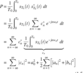
According to the Parseval’s theorem, the power of a periodic signal may be expressed in terms of the Fourier series coefficients:
P= 1
One may also observe from (1.5) that the power of a periodic signal is equal to the sum of the powers |cn|2of its spectral components, located at nf0, and its PSD is discrete with values |cn|2. Hence, the signal power is the same irrespective of whether it is calculated in time-or frequency-domains.
Example 1.1 Fourier Series of a Rectangular Pulse Train.
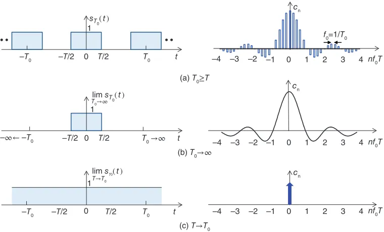
Consider the rectangular pulse train shown in Figure 1.1. Using (1.3) we determine the com-plex Fourier series ofsT0 t :
Being a damped sinusoid, the zeros of the sinc function are the same as those of the sine function, that is, x= ±1, ±2,..., except for at x= 0 where it is equal to unity:
sinc n =δn, n= 0, ± 1, ± 2, (1.8)
Figure 1.1(a) shows the variation ofcnas a function ofnf0T. Note that asT0goes to infinity as in Figure 1.1(b), the periodic rectangular pulse train reduces to a single pulse at the origion. Then, the spectral lines merge, that is, f0 0, and the discrete spectra shown in Figure 1.1(a) becomes continuous and is described by sinc(fT) whose zeros are given by k/T, k= 1, 2,…. On the other hand, as T0 T we have sT0 t = 1 (see Figure 1.1(c))
and the corresponding Fourier coefficients become
1.1.2
Fourier Transform
AsT0goes to infinity as shown in Figure 1.1(b), sT0 t tends to become an aperiodic signal,
which will be shown hereafter as s(t). Then,f0= 1/T0approaches zero, spectral lines atnf0merge and form a continuous spectrum. The Fourier transform S(f) of an aperiodic continuous functions(t) is defined by [2][3][9]
S f =ℑs t =
This Fourier transform relationship will also be denoted as
s t S f (1.11)
Unless otherwise stated, small-case letters will be used to denote time-functions while capital letters will denote their Fourier trans-forms. It is evident from (1.10) that the value
of S(f) at the origin gives the mean value of The so-called Rayleigh’s energy theorem states that the energy of an aperiodic signal found in time- and frequency-domains are iden-tical to each other:
E=
In view of the integration over−∞<f<∞in (1.13), the energy of s(t) is equal to the area under the energy spectral densityΨs(f) ofs(t), that is, the energy per unit bandwidth:
Ψs f = S f 2, J Hz (1.14)
One may observe from (1.10) that the Fourier transform, hence the ESD, of a real signal s(t) with even symetry s(t) =s(−t), has also even symmetry with respect tof= 0.
Example 1.2 Fourier Transform of a Rectangular Pulse.
Lets(t) be defined as
s t =AΠ t T =A 1 t <T 2
0 t >T 2 (1.15)
whereAis a constant. Using (1.10), the Fourier transform of (1.15) is found as follows:
S f =A
T 2
−T 2 e−jwtdt
=AT sinc fT
(1.16)
where sinc(x) is defined by (1.7) (see (1.6) and Figure 1.1(b)).
Figure 1.2(a) shows the Fourier transform rela-tionship between the (1.15) and (1.16). The frequency components of the pulse, which is time-limited to ±T/2, extends over (−∞, ∞) in the frequency domain. In the limiting case whereT ∞, then the pulse extends uniformly over (−∞,∞) in the time domain, hence a dc sig-nal (band-limited but not time-limited). Then, the pulse can be represented by only a single frequency component atf= 0, hence by a delta function, in the frequency domain (see Figure 1.2(b)). On the other hand, if we let A = 1/Tso that the area under the pulse becomes unity (see Figure 1.2(c)), and letT 0, then the time-limited pulse approaches a delta function and its Fourier transform S(f) tends to be flat in the frequency domain. As one may also observe from the Fourier transform relationship in (1.10), a time-limited signal has frequency components over (−∞,∞), hence not band-limited, while a band-limited signal can not be time-limited. To have a better feeling about the time-frequency relationship, we observe from Figure 1.2(a) that the bandwidth between dc and the first null of the sinc function is given byW= 1/T. If we use this bandwidth as a measure of the spectrum occupancy of the pulses(t), the product of the pulse durationT and the bandwidth isWT= 1.
s(t)
–T/2 0 T/2 t A
0 f
1
0 t
A=1/T
0 f
S(f)=A δ(f)
S(f)
–4 –3 –2 –1 0 1 2 3 4 f T
0 t
A s(t)
s(t)
S(f)=AT sinc(fT)
(a) 0<T<∞
(b) T → ∞
(c) T → 0
In general, the so-called time-bandwidth product, which relates time and frequency behaviors of a signal, is a constant and its value depends on the considered pulse. This implies that bandwidth and the pulse duration are inversely related to each other. Hence, faster changing pulses, that is, pulses with smallerT, occupy wider band-widths. In other words, higher data rate transmis-sions require wider transmission bandwidths. Indeed, high data rate transmissions (with min-imum pulse durations) in minmin-imum possible transmission bandwidths is one of the challen-ging issues in telecommunications engineering.
1.1.2.1 Impulses and Transforms in the Limit
Dirac delta function does not exist physically, but is widely used in many areas of engineer-ing. Some functions are used to approximate the Dirac delta function. For example, the rect-angular pulse shown in Figure 1.2 approxi-mates Dirac delta function in the time domain asTapproaches zero. As the area under a Dirac delta function should be equal to unity, the amplitude of the rectangular pulse is chosen asA= 1/T. Figure 1.2(c) also shows that a Dirac delta function in the time domain has a flat spectrum, that is, its PSD is uniform. Similarly, the Fourier transform of a rectangular pulse approximates a Dirac delta function located at f= 0 asT ∞(see also Figure 1.2(b)), which implies that the Dirac delta function in the fre-quency domain implies a time-invariant signal. Some alternative definitions of the Dirac delta function are listed below: [2][3][9]
δt−t0 =
∞ t=t0
0 t t0
δt = lim
T 0
1 TΠ
t T δ f = lim
T ∞T sincfT
δt−t0 = ∞
−∞
e±j2πt−t0λ
dλ
(1.17)
Some properties of the Dirac delta function are summarized below:
a. Area under the Dirac delta function is unity:
∞
−∞
δt−t0 dt= 1 (1.18) b. Sampling of an ordinary functions(t) which
is continuous att0:
b a
s t δt−t0 dt=
s t0 a<t0<b s t0 2 t0=a, t0=b
0 otherwise (1.19)
c. Relation with the unit step function
u t−t0 =
t
−∞
δ τ−t0 dτ=
1 t>t0
1 2 t=t0
0 t<t0
δ t−t0 = d dtu t−t0
(1.20)
d. Multiplication and convolution with a con-tinuous function:
s t δ t−t0 =s t0 δt−t0
s t δt−t0 =s t−t0 (1.21) e. Scaling
δat = 1
aδ t (1.22)
f. Fourier transform
δ t∓t0 e∓jwt0
e±jw0t δ f∓f0 (1.23)
1.1.2.2 Signals with Even and Odd Symmetry and Causality
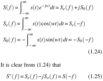
S f = ∞
−∞s t e
−jwt
dt=Se f +jS0 f
Se f =
∞
−∞s t cos wt dt=Se −f
S0 f =−
∞
−∞
s t sin wt dt=−S0 −f (1.24)
It is clear from (1.24) that
S∗ f =S
e f −jSo f =S −f (1.25)
When the signal has an even symmetry with respect to t= 0, that is, s(t) =s(−t), then S(f) becomes a real and even function of frequency:
S f =Se f = 2
∞
0
s t coswt dt
So f = 0
(1.26)
When the signal has an odd symmetry with respect to t= 0, that is,s(t) =−s(−t), then S(f) becomes a purely imaginary and odd function of frequency:
S f =jSo f =−j2
∞
0
s t sin wt dt
Se f = 0
(1.27)
Acausal systemis defined as a system where the output at timet0depends on only past and current values but not on future values of the input. In other words, the outputy(t0) depends only on the inputx(t) for values oft≤t0. There-fore, the output of a causal system has no time
symmetry and its spectrum has both real and imaginary components.
Example 1.3 Fourier Transform of a Decay-ing Exponential Function.
Consider a decaying exponential function as shown in Figure 1.3. Its Fourier transform is obtained using (1.10) and (1.20) as follows:
s t =e−αtu t, α> 0 S f =1 2δ f +
1
α+jw (1.28)
We can use (1.28) to rewrite the unit step function as follows:
u t = lim
α 0 s t (1.29)
The Fourier transform of the unit step func-tion may then be expressed as follows:
U f =ℑ u t = lim α 0ℑ s t
= lim α 0
1 2δ f +
1
α+j2πf =1
2δ f + 1
j2πf (1.30)
Based on (1.10) and (1.28), the following Fourier transform pairs are valid forα> 0:
s −t S −f =1 2δ f +
1
α−jw s t −s −t S f −S −f =−j 2w
α2+w2
(1.31)
s(t)
0 t
1
0 f
1/α |S(f)|
0.5 δ(f)
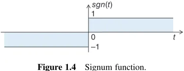
The signum function may be defined in terms of the unit step function as follows (see Figure 1.4):
sgn t =u t −u −t
= lim α 0 s t
−s −t =
1 t> 0 0 t= 0 −1 t< 0
(1.32)
The Fourier transform of the signum func-tion, which has an odd symmetry, is found using (1.30) and (1.31):
ℑsgnt =U f −U −f
= lim
α 0 S f −S −f =
1
jπf (1.33) which is purely imaginary, as expected (see (1.27)).
1.1.2.3 Fourier Transform Relations Some properties of the Fourier transform are listed below: [2][3][9]
a. Superposition
Ifsi t Si f , i= 1,2, , then using the
linearity property of the Fourier transform in (1.10),
s t =
i
αisi t S f = i
αiSi f
(1.34)
b. Time and frequency shift Ifs t S f , then
s t∓τ S f e∓jwτ s t e±jwct S f∓f
c
(1.35)
Proof: The use of variable transformations in the following equations lead to
ℑs t∓τ =
∞
−∞
s t∓τ e−jwtdt=e∓jwτS f
ℑs t e±jwct =
∞
−∞
s t e−j w∓wc tdt=S f∓f c
(1.36)
Example 1.4 Frequency Translation and Modulation.
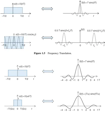
Consider the rectangular pulse and its Fourier transform given by (1.15) and (1.16). From (1.35), one can write
Π t T T sinc fT
Π t T e±jwct T sinc f∓f c T
(1.37)
One may easily observe from (1.37) that multiplying a time function by an exponential term exp(jwct) simply shifts the center fre-quency of the signal spectrum from dc to fc. One may use linearity property, given by (1.34), to obtain the following from (1.37):
Π t T cos wct
T
2 sinc f+fc T +T
2 sinc f−fc T (1.38) Figure 1.5 shows the effect of multiplying a rectangular pulse by a sinusoidal carrier with fre-quencyfc. Multiplying a rectangular pulse with cos(wct) with−∞<t<∞makes cos(wct) time-limited to–T/2 <t<T/2. This operation, which results in shifting the spectrum of the rectangular pulse from dc to ±fc, is widely used in transmit-ters for upconverting baseband signals to higher frequencies for passband transmission. Here, it is important to note that the passband signals occupy twice the transmission bandwidth com-pared to baseband signals due to the fact that negative frequency components of the baseband signals are also shifted around the carrier fre-quency (see Figure 1.5(b)). As we shall see in
0 t
1
–1 sgn(t)
the subsequent chapters, multiplication of the bandpass signal Π(t/T)coswct by a carrier of the same frequency restores the baseband signal at the receiver, since EΠt T cos2w
ct =
1 2Π t T . Here, the expectation operation may be implemented by a low-pass filter.
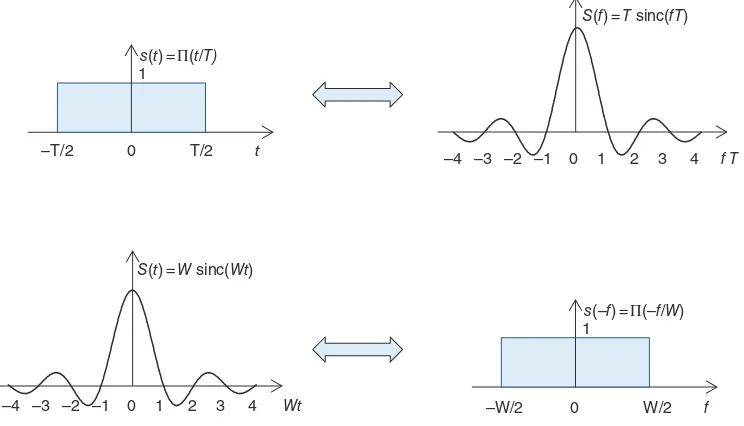
c. Time and frequency scaling
Ifs t S f , then, for a real numberα,
s αt α −1S f α (1.39)
Proof:
ℑsαt =
∞
−∞
sαt e−jwtdt =α−1
∞
−∞s
αt e−j wα αt αdt = α−1S f α
(1.40)
As shown in Figure 1.6, s(αt) is com-pressed in time compared tos(t) by a factor
α> 1. However, S(f/α) is expanded in fre-quency by the same factor. Compression in
0 f
S(f) =T sinc(fT) s(t) =Π(t/T)
–T/2 0 T/2 t
s(t) =Π(t/T) cos(wct)
–T/2 0 T/2 t –fc 0 fc f
S(f)
0.5 T sinc((f–fc)T) 0.5 T sinc((f+fc)T)
Figure 1.5 Frequency Translation.
s(t) =Π(t/T)
–T/2 0 T/2 t
1
–4 –3 –2 –1 0 1 2 3 4 f T
–4 –3 –2 –1 0 1 2 3 4 f T S(f) =T sinc(fT)
s(t) =Π(αt/T)
–T/(2α) 0 T/(2α) t 1
S(f) = (T/α) sinc(fT/α)
the time domain, that is, faster variation of the signal with time, implies an expansion of its Fourier transform in the frequency domain, that is, the signal occupies a larger band-width. However, the time bandwidth product remains the same; αW T α =WT. d. Duality
Ifs t S f , then
S t s −f (1.41)
Proof: First changing the sign of t and interchangingtandfleads to
s −t = ∞
−∞
S f e−j2πftdf
s −f = ∞
−∞
S t e−j2πftdt S t s −f
(1.42)
Example 1.5 Duality.
Using the Fourier transform relationship given by (1.15) and (1.16), one can write from (1.41)
s t =Π t T S f =T sinc fT
S t =W sinc W t s −f =Π −f W (1.43)
by interchangingT withW in the second line (see Figure 1.7).
e. Conjugation
Ifs t S f then
s∗ ±t S∗ ∓f (1.44)
Proof:
s∗ t =
∞
−∞
S∗ f e−jwtdf
=
∞
−∞
S∗ −f ejwtdf S∗ −f
s∗ −t =
∞
−∞
S f e−jwtdf
∗
=
∞
−∞
S∗ f ejwtdf S∗ f
(1.45)
f. Convolution
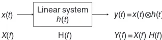
Ifs t S f andr t R f , then
r t s t R f S f
r t s t R f S f (1.46)
s(t) =Π(t/T)
–T/2 0 T/2 t
1
f T S(f) =T sinc(fT)
s(–f) =Π(–f/W)
–W/2 0 W/2 f
1
–4 –3 –2 –1 0 1 2 3 4
–4 –3 –2 –1 0 1 2 3 4
Wt S(t) =W sinc(Wt)
where denotes the convolution operator:
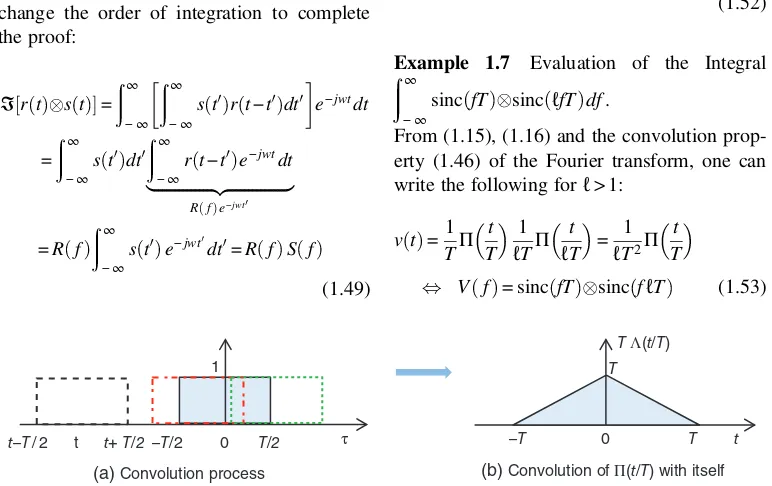
Proof: Inserting the Fourier transform ofr(t) into the first line of the following and interchan-ging the order of integration completes the proof of the first line of (1.46):
ℑr t s t =
Similarly, we first write the convolution inte-gral in the Fourier transform expression and change the order of integration to complete the proof:
Example 1.6 Fourier Transform of a Tri-angular Waveform.
Figure 1.8 shows that the convolution of a pulse of durationTwith itself yields a triangular pulse in (−T,T) with an amplitudeT:
where the triangular waveform is defined as:
Λ t τ = 1− t τ t <τ
0 otherwise (1.51)
Using (1.15), (1.16) and (1.46), Fourier trans-form of a triangular wavetrans-form is found to be
Π t T T sinc fT
Λ t T =1
TΠ t T Πt T T sinc 2 fT
(1.52)
Example 1.7 Evaluation of the Integral ∞
−∞
sincfT sinc ℓfT df.
From (1.15), (1.16) and the convolution prop-erty (1.46) of the Fourier transform, one can write the following forℓ> 1:
v t =1
From (1.12), the integral of the convolution
Using (1.12) and the Fourier transform rela-tionship given by (1.15) and (1.16), one gets
∞
Proof: Noting that differentiation is not with respect to the variable of integration, one can easily find
Note that the differentiation with respect to time enhances the high-frequency components of a signal since j2πf nS f > S f for
2πf > 1 [2].
Example 1.8 Fourier Transform of a Tri-angular Waveform Using the Differentiation Property.
We use differentiation property to determine the Fourier transform of a triangular waveform defined by (1.51). Using (1.56), we can express the Fourier transform of a triangular wave-form as
The first two time-derivatives of a triangular waveform may be written as (see also Figure 1.9)
The second derivative of a triangular wave-form may be expressed in terms of Dirac delta functions, whose Fourier transform is straight-forward. Inserting the second derivative of Λ(t/T) in (1.59) into (1.58) and using (1.23),
ℑΛ t T = 1
which is identical to (1.52), as expected.
h. Integration Proof: The above integral may be expressed as the convolution of s(t) with the unit step
The use of (1.30) and the convolution prop-erty given by (1.46) leads to (1.61). Note that the integration of a function suppresses its high-frequency components since S f 2πf
<S f for |2πf| > 1 [2].
Example 1.9 Fourier Transforms of the Unit Step and the Dirac Delta Functions Using Inte-gration and Differentiation Properties. In view of (1.20), (1.23), (1.30) and (1.61), one Fourier transform of a delta function may be determined using the differentiation property as follows
which is the same as (1.23), as expected.
1.1.3
Fourier Transform of Periodic
Functions
Fourier transform of a periodic function, of periodT0, with a complex Fourier series expan-sion given by (1.3) is given by [4]
The Fourier transform (1.65) is hence a dis-crete function of frequency, that is, is non-zero at only the discrete frequencies nf0. The PSD may be written as the square of the magnitude of its Fourier transform:
Gs f = ℑsT0 t
The power of a periodic signal is given by the area under the PSD:
P=
Similarly, as given by (1.6) and shown in Figure 1.1, the coefficients of the complex Fourier series expansion of a periodic rectangu-lar pulse train, with period T0= 1/f0, also exhibit discrete frequency lines. One may observe from (1.6) that the coefficients satisfy cnT0=S nf0 where S(f) denotes the Fourier
transform of a single rectangular pulse centered at the origin (see (1.15), (1.16) and the pulse train sT0 t as T0 ∞ in Figure 1.1(b)). The
PSD and the power of a periodic signal, given by (1.5), determined by the Fourier series ana-lysis, are in complete with agreement with (1.66) and (1.67), found by the Fourier trans-form approach.
Gs f = lim
Example 1.10 Fourier Transform of a Peri-odic Train of Impulses in Time.
Consider the following periodic discrete-time function, which consists of a periodic train of impulses with periodT:
sT t =
∞
m=−∞
δ t−mT (1.69)
Using (1.3) withf0= 1/T, the complex Fou-rier series expansion of (1.69) may be written as follows:
The Fourier transform of the RHS of (1.70) with cn= 1/T, as given by (1.65), shows that the Fourier transform of a train of impulses with periodTin the time domain consists of a train of impulses in the frequency domain separated from each other by 1/T:
In digital communication systems, the first step of converting analog signals into digital, is to sample analog signals. Consider the following discrete-time function which represents the sequence of samples of an analog signal g(t) with a sampling period ofT(see Figure 1.10):
gδ t =g t
∞
m=−∞
δ t−mT (1.73)
Since the sampled analog signalgδ(t) may be
written as the product ofg(t) and the periodic sequence of Dirac delta functions, its Fourier transform Gδ(f) may be expressed, using
(1.72), as the convolution of their Fourier trans-forms in the frequency domain:
gδ t =g t
1.2
Power Spectal Density (PSD)
and Energy Spectral
Density (ESD)
1.2.1
Energy Signals Versus
Power Signals
The energy of a signals(t) is defined as
E= ∞
−∞
s t 2dt (1.75)
The power of a signal is defined as
P= lim
T ∞ 1 T
T 2
−T 2
s t 2dt (1.76)
As a special case when the power signal is periodic with a period T0, the signal power defined by (1.76) simplifies to
P= 1 T0
T0 2
−T0 2 sT0 t
2
dt (1.77)
Based on (1.75)−(1.77), signals may be clas-sified as
a. An energy signal is defined as a signal with finite energy and zero power:
0 <E<∞ P= 0 (1.78)
Aperiodic signals are typically energy sig-nals as they have a finite energy and zero power.
b. A power signal has finite power and infinite energy:
0 <P<∞ E=∞ (1.79)
Periodic signals are typically power signals since they have finite power and infinite energy. [4][5][6][7]
Example 1.12 Energy and Power Signals. Let us first consider the following decaying exponential function:
s t =Ae−αtu t , α≥0 (1.80) whereu(t) denotes the unit step function andα
is a positive finite real number. The energy and
0 t –W/2 0 W/2 f
G(f) g(t)
–4 –3 –2 –1 0 1 2 3 4 t/T
δ(f−n/T) δ(t−mT)
m=−∞ ∞
∑ 1
n=−∞ T
∞ ∑
–2 –1 0 1 2 fT
gδ(t) Gδ(f)
| |
× ⊗
= =
| |
• • • • • •
• • • • • •
• • •
• • • • • •
• • •
–4 –3 –2 –1 0 1 2 3 4 t/T
–2 –1 0 1 2 fT
power of this signal are calculated using (1.75) and (1.76) as follows:
E= Hence, this is an energy signal. However, if we assume A = 1 andα= 0 in (1.80), then
which shows that a unit step function is a power signal.
Now consider the following signal:
s t = t
−1 4 t≥t 0> 0
0 elsewhere (1.83)
Its energy and power are found to be
E=
This signal is neither a power signal nor an energy signal.
Finally we consider a cosine function with amplitudeA:
sT0 t =Acos w0t+θ (1.85)
Since this function is periodic with a period T0= 1/f0, its power can be determined by inte-gration over one period:
P= 1
The energy of this signal is given by the product of its power and the number of periods
considered, which is infinite. Therefore, this signal having infinite energy, is classified as a power signal.
1.2.2
Autocorrelation Function and
Spectral Density
ESD and PSD are employed to describe the dis-tribution of, respectively, the signal energy and the signal power over the frequency spectrum. ESD/PSD is defined as the Fourier transform of the autocorrelation function of an energy/ power signal. [4][5][6][7]
1.2.2.1 Energy Signals
Autocorrelation of a function s(t) provides a measure of the degree of similarity between the signal s(t) and a delayed replica of itself. The autocorrelation function of an energy sig-nals(t) is defined by measures the time shift between s(t) and its delayed replica. The sign of the time shiftτshows whether the delayed version ofs(t) leads or lags s(t). If the time shiftτbecomes zero, thens(t) will overlap with itself and the resemblence between them will be perfect. Consequently, the value of the autocorrelation function at the origion is equal to the energy of the signal:
E=Rs 0 =