Dynamic Whole Body Motion Generation Under Rigid Contacts and Other Unilateral Constraints06482266

Dynamic Whole-Body Motion Generation Under

Rigid Contacts and Other Unilateral Constraints

Layale Saab, Oscar E. Ramos, Franc¸ois Keith, Nicolas Mansard, Philippe Sou`eres, and Jean-Yves Fourquet

Abstract_{—The most widely used technique for generating}

whole-body motions on a humanoid robot accounting for various tasks and constraints is inverse kinematics. Based on the task-function approach, this class of methods enables the coordination of robot movements to execute several tasks in parallel and account for the sensor feedback in real time, thanks to the low computation cost. To some extent, it also enables us to deal with some of the robot con-straints (e.g., joint limits or visibility) and manage the quasi-static balance of the robot. In order to fully use the whole range of possible motions, this paper proposes extending the task-function approach to handle the full dynamics of the robot multibody along with any constraint written as equality or inequality of the state and control variables. The definition of multiple objectives is made possible by ordering them inside a strict hierarchy. Several models of contact with the environment can be implemented in the framework. We propose a reduced formulation of the multiple rigid planar contact that keeps a low computation cost. The efficiency of this approach is illustrated by presenting several multicontact dynamic motions in simulation and on the real HRP-2 robot.

Index Terms_{—Contact modeling, dynamics, force control,}

humanoid robotics, redundant robots.

I. INTRODUCTION

T

HE generation of motion for humanoid robots is a chal-lenging problem, due to the complexity of their tree-like structure and the instability of their bipedal posture [3]. Typi-cal examples are shown in Fig. 1, with the HRP-2 robot using multiple non-coplanar contacts to perform a dynamic motion. These robots own a large number of degrees of freedom (DOFs),

Manuscript received July 19, 2012; accepted December 11, 2012. Date of publication March 20, 2013; date of current version April 1, 2013. This paper was recommended for publication by Associate Editor Y. Choi and Editor B. J. Nelson upon evaluation of the reviewers’ comments. This paper was presented in part at the IEEE International Conference on Robotics and Automation in 2011 [1] and the IEEE/RSJ International Conference on Intelligent Robots and Systems in 2011 [2].

L. Saab was with the Laboratory for Analysis and Architecture of Systems, Centre National de la Recherche Scientifique, University of Toulouse, Toulouse F-31400, France. She is now with EOS Innovation, ´Evry 91000, France (e-mail: layalesaab@gmail.com).

O. E. Ramos, N. Mansard, and P. Sou`eres are with the Laboratory for Anal-ysis and Architecture of Systems, Centre National de la Recherche Scien-tifique, University of Toulouse, Toulouse F-31400, France (e-mail: oscarefrain@ gmail.com; nicolas.mansard@laas.fr; soueres@laas.fr).

F. Keith is with Laboratoire d’Informatique de Robotique et de Mi-cro´electronique de Montpellier, Montpellier 34095, France. He is also with CNRS-AIST Joint Robotics Laboratory, UMI3218/CRT, Tsukuba, Japan (e-mail: francois.keith@lirmm.fr).

J-Y. Fourquet is with the Laboratoire G´enie de Production, de l’Ecole Na-tionale d’ Ing´enieurs de Tarbes, University of Toulouse, Tarbes 65016, France (e-mail: fourquet@enit.fr).

Color versions of one or more of the figures in this paper are available online at http://ieeexplore.ieee.org.

Digital Object Identifier 10.1109/TRO.2012.2234351

Fig. 1. Dynamic multicontact motion with the HRP-2 model.

typically more than 30. In return, they are subject to various sets of constraints (balance, contact, actuator limits), which reduce the space of possible motions. These constraints can typically be formulated as equalities (e.g., zero velocity at rigid-contact points [4]), and inequalities (e.g., joint limits [5], obstacles [6], joint velocity and torque within given bounds). Moreover, they are of relative importance (e.g., balance has to be considered more important than visibility [7]). In total, the motion has to be designed in a set that lives in the high-dimensional configuration space but is implicitly limited to a much smaller submanifold by the set of constraints. This makes the classical sampling methods [8], [9] more difficult to use than for a classical ma-nipulator. The motion manifold cannot be sampled directly but by projection [10]. The connection process in high-dimension is costly [11] and often fails due to the number of constraints.

Rather than designing the motion at the whole-body level (configuration space), the task function approach [12], [13] pro-poses designing the motion in a space dedicated to the task to be performed. It is then easier to design the reference motion in the task space, and transcripting this reference from the task space to the whole-body level is only a numerical problem. This approach is versatile, since the same task is generally transpos-able from one robot or situation to another. It also eases the use of sensory feedback, since the sensory space is often a good task-space candidate [14], [15].

A task is a basic brick of motion, which can be combined se-quentially [16] or simultaneously to a complex motion. Simul-taneous execution can be achieved in two ways: by weighting, or by imposing a strict hierarchy. Coming from numerical op-timization [17], this second solution was introduced in robotics by [18] and formalized for any number of tasks in [19], [20]. This approach is well fitted to cope with equality constraints. However, inequality constraints cannot be taken into account explicitly. Therefore, approximate solutions, such as potential field approaches [7], [22] or damping functions [5], [23] have been proposed to consider inequalities.

The transcription of the motion reference from the task space to the whole-body control is naturally written as a quadratic

program (QP) [24]. A QP is composed of two layers, namely the constraint and the cost. It can be seen as a hierarchy of two levels, the constraint having priority over the cost. If only equality constraints are considered, the QP resolution corre-sponds to the inversion schemes [20], in the particular case of two levels. Inequalities can also be taken into account directly, as constraints, or in the cost function [25]. In [26], a method to extend the QP formulation to any number of priority levels is given. The solution of such a hierarchical problem is computed by solving a cascade of QP (or hierarchical QP). In [27], a dedi-cated solver has been proposed to obtain the solution in one step inside a cascade, which reduces the cost.

All these works only consider the kinematics of the robot. On a humanoid robot, many constraints arise from the dynamics of the multibody system. The formulation by task can be extended to compute the torque at the whole-body level from the reference motion expressed in the dedicated task space, which is also calledoperational space[28]. For a humanoid in contact, the motion is constrained to the submanifold of configurations that respects the contact model [29], as illustrated in Fig. 1. A review of the work in modeling and control of the dynamics of a set of bodies in contact is proposed in [30] and [31]. The connection with inverse dynamics has been done in [32] and [33]. Using these approaches, it is possible to take into account a hierarchy of tasks and constraints (orstackof tasks [34]), all written as equalities [35], [36]. In [37], a first solution to handle inequalities in the stack of tasks (SOT) was proposed, but cannot set any inequality constraint on the contact forces. In [38] and [39], the inverse-dynamics problem has been written as a QP, where the unilateral contact constraints, along with classical unilateral constraints (joint limits, etc.) are explicitly considered. In that case, several tasks can be composed by setting relative weights, but a hierarchy of tasks is not possible.

In this paper, we propose a generic solution for taking into account equalities and inequalities in a strict hierarchy to gen-erate a dynamic motion. This solution is based on the simi-larities between inverse kinematics and inverse dynamics. In Section II, the inverse-kinematics scheme is recalled, written into a general form; the possibility of taking into account in-equalities is then introduced using the solver [26], [27]. Then, putting the operational-space inverse dynamics under the same generic form, Section III uses the same hierarchical solver to take into account both dynamics and inequalities. This first so-lution deals with the robot in free space. In Section IV, con-tacts are introduced in the model and used in the resolution scheme. The contact model is generic and can be adapted to various situations (rigid contact, friction cone [40], elastic con-tact [41]). A solution is proposed in Section V for implement-ing a reduced form of multiple plane/plane slidimplement-ingless rigid contacts. In Section VI, the connection is made with the zero-moment point (ZMP) contact criterion [42] classically used in humanoid robotics [43]. The generation is close to the real time (around 20 ms per control cycle on a typical 30-DOF robot). Some examples of complex motions involving noncoplanar contacts and their execution on the real robot are presented in Section VII.

II. INVERSEKINEMATICS

A. Task-Function Approach

The task-function approach [13], or operational-space ap-proach [28], [44], provides a mathematical framework for de-scribing tasks in terms of specific output functions. The task function is a function from the configuration space to an arbi-trary task space, which is chosen to ease the observation and the control of the motion with respect to the task to perform.

A task is defined by a triplet(e,e˙∗, Q), whereeis the task function that maps the configuration space to the task space and

˙

e∗_{is the reference behavior expressed in the tangent space to the}

task space ate.Qis the differential mapping between the task space and the control space of the robot that verifies the relation

˙

e+μ=Qu (1)

where uis the control in the configuration space andμis the drift of the task. To compute a specific robot control u∗ that performs the referencee˙∗, any numerical inverse ofQcan be used. The generic expression of the control law is then

u∗=Q#( ˙e∗+μ) +Pu2. (2)

In this expression, the first part performs the task, and the sec-ond part, modulated by the secsec-ondary control input u2, ex-presses the redundancy of the task [18]. In the first term,Q#

is any reflexive generalized inverse of Q, often chosen to be the (Moore–Penrose) pseudoinverseQ+ [45] or a weighted in-verseQ#W [46] (see Appendix A). In the second term of (2),

P=I₋Q#Qis the projector onto the null space ofQ corre-sponding toQ#.

B. Hierarchy of Tasks

The projectorPis intrinsically related to the redundancy of the robot with respect to the taske. A secondary task(e2,e˙∗2, Q2) can be executed usingu2as a new control input. Introducing (2) ine˙2+μ2 =Q2ugives

˙

e2+ ˜μ2 =Q2u2 (3)

withμ˜2 =μ2−Q2Q#( ˙e∗+μ)andQ2 =Q2P. This last equa-tion fits the template (1), and can be solved using the generic expression (2) [20]

u∗₂ =Q2 #

( ˙e∗+ ˜μ2) +P2u3 (4)

whereP2 enables the propagation of the redundancy to a third task using the inputu3. By recurrence, this generic scheme can be extended to any arbitrary hierarchy of tasks.

C. Inverse Kinematics Formulation

In the inverse-kinematics problem, the control inputuis sim-ply the robot joint velocityq˙. The differential mapQbetween the task and the control is the task JacobianJ. In that case, the driftμ= ∂ e_{∂ t} is often null, and (1) is written as

˙

The simplest and most-often used solution is to chooseQ# to be the pseudoinverseQ+, which gives the least Euclidean norm of bothq˙ande˙∗_{−Jq˙[47], [48]. The control law is then}

˙

q∗ = ˙q₁∗+Pq˙2 (6)

whereq˙∗

1 =J+e˙∗. A typical reference behavior is an exponential decay ofeto zeroe˙∗₌₋λ_e,λ_>0.

It may happen that J becomes singular, i.e., rank(J)< r0, wherer0is the nominal rank ofJout of the singular configura-tion. Numerical problems can occur during the transition from the nominal situation to the singular one. To avoid these prob-lems, the pseudoinverse is often approximated by the damped least-squareJ†defined by [49], [50]

J†=

_J

ηI

+

I 0

(7)

whereIis the identity matrix of proper size, andηis a damping factor, chosen as an additional parameter of the control (typi-cally,η=10−2for a humanoid robot).

D. Projected Inverse Kinematics

Consider a secondary task(e2,e˙∗2, J2). The template (3) is written as

˙

e2−J2q˙∗1=J2Pq˙2. (8)

In this case, the differential map is the projected JacobianQ= J2P, and the drift isμ=−J2q˙∗1. The control inputq˙2∗is obtained once more by numerical inversion [20], [21]

˙

q2∗= (J2P)+( ˙e2 −J2q˙∗) +P2q˙3 (9)

whereP2 is the projector into the null space ofJ2P. The same scheme can be reproduced iteratively to take into account any number of tasks untilPiis null.

In general, rank(J2P)≤rank(J2)≤r2, wherer2is the nom-inal rank ofJ2. When the second inequality is strict, the sin-gularity is said to be kinematic; when the first inequality is strict, the singularity is said to bealgorithmic[51].1 _{To avoid} any numerical problem in the neighborhood of the singularity, a damped inverse can be used to invertJ2P.

E. Hierarchical Quadratic Program Resolution

1) Generic Formulation: When considering a single task, the solution obtained with the pseudoinverse (2) is known to be the optimal solution of the QP min

u Qu−e˙

∗_−μ2_{. The great} advantage of the QP formulation is that both linear equalities and inequalities can be considered, while the pseudoinverse-based schemes presented previously cannot explicitly deal with inequalities. A QP is composed of a quadratic cost function to be minimized, while satisfying the set of constraints [52]. It can be seen as a two-level hierarchy, where the set of constraints has priority over the cost. Inequalities are set as the top priority. The introduction of slack variables is a classical solution to handle

1_{Both cases are similar in the sense that[}J1

J2]is singular.

an inequality at the second priority level [53]. In [26], use of the slack variables was proposed to generalize the QP to more than two levels of hierarchy and, thus, to build a hierarchical quadratic problem (HQP) handling inequalities.

The HQP formulation is first recalled in a generic frame. A generic constraintkis defined by the linear mapAk and the two

inequality bounds(b_k, bk), whereb_k andbk are, respectively,

the lower and upper bounds on the reference behavior.2_{At level}

k, the cascade algorithm that solves the hierarchy (Ak, bk)is

expressed by the following QP:

min

uk,wkwk

2

s.t. b

k₋1 ≤Ak−1uk +w ∗

k₋1 ≤bk₋1

b_{k ≤}Akuk+wk ≤bk (10)

whereAk₋1,(b_k

−1,bk−1)are the constraints at all the

previ-ous levels from 1 tok₋1(Ak₋1 = (A1, . . . , Ak−1)), andAk,

(b_k, bk)is the constraint at levelk.

The slack variable3 wk is used to add some freedom to the

solver if no solution can be found when the constraintkis in-troduced under thek−1 previous constraints:wk is variable

and can be used by the solver to relax the last constraintAk.

On the other hand,w_k∗

−1is constant and set to the result of the

previous optimization of thek₋1 first QP (at each of the itera-tions of the cascade,w∗_k

−1is augmented with the optimalw∗_kby w∗_k

−1 := (w∗k₋1, w_k∗)). A solution to thestrictk−1 constraint Ak₋1is then always reached, even if theslackconstraintA_kis

not feasible. This corresponds to the definition of the hierarchy. A classical method to compute the solution of a QP or HQP relies on an active-search algorithm [27], [52] (see Appendix B), which implies iterative computations of the pseudoinverse of a subproblem of the initial QP. Since pseudoinverses are used, the classical numerical problems can occur in the neighborhood of singularities. Regularization methods that extend the damping inverse [50] used in robotics can be applied [54].

The method proposed previously is generic and can be ap-plied to any numerical problem written with a linear hierar-chical structure. In that case, it is referred to as HQP (or cascade of QP) and denoted with the lexicographic order:

(i)≺(ii)≺(iii)≺. . .which means that the constraint(i)has the highest priority. In the following, we propose a solution to apply this formulation to invert kinematics and dynamics. The constraints are then the tasks defined previously, and the hierarchical solver will be called an SOT or hierarchy of tasks.

2) Application to Inverse Kinematics: When considering a single task, inversion (6) corresponds to the optimal solution to the problem

min ˙

q Jq˙−e˙

∗2_{. (11)}

2_{Specific cases can be immediately implemented.b}

k=bk in the case of equalities andb_k=−∞orbk= +∞to handle single-bounded constraints.

By applying the QP resolution scheme, both equalities and in-equalities can be considered. Replacingb by e˙, the reference part is then rewritten as

˙

e∗≤e˙ ≤e˙∗. (12) For instance, in the case of two tasks with priority ordere1 ≺e2, the expression of the QP is given by

min ˙

q ,w2 w22

s.t. e˙∗_{1 ≤}J1q˙+w1∗≤e˙

∗

1

˙

e∗_{2 ≤}J2q˙+w2 ≤e˙∗2. (13) In robotics, when a constraint is expressed as an inequality, it is very likely to be put as the top priority: typically, joint limits and obstacle avoidance. Using this framework, it is also possible to handle inequalities at the second priority level (i.e., in the cost function). A typical case is to prevent visual occlusion when possible, or to keep a low velocity if possible, without disturbing the robot behavior when it is not necessary.

In the sequel, the HQP considering linear equalities and in-equalities will be extended from inverse kinematics to inverse dynamics.

III. INVERSEDYNAMICS

In this section, the case of a contact-free dynamical multibody system without free-floating root is considered.

A. Task-Space Formulation

As previously stated, a task is defined by a task functione, a reference behavior, and a differential mapping. At the dynamic level, the reference behavior is specified by the expected task acceleration ¨e∗, while the control input is typically the joint torquesτ. The operational-space inverse dynamics then refers to the problem of finding the torque control inputτthat produces the task reference¨e∗, using any necessary joint accelerationq¨. The acceleration q¨is then a side variable that does not have to be explicitly computed during the resolution. Contrary to the case of kinematics, the mapping between the control inputτand the task space is obtained in two stages. First, the map between accelerations in the configuration space and in the task space is obtained by differentiating (5)

¨

e=Jq¨+ ˙Jq.˙ (14) Then, the dynamic equation of the system expressed in the joint coordinates is deduced from the mechanical laws of motion [55]

A¨q+b=τ (15)

whereA=A(q)is the generalized inertia matrix of the system,

¨

qis the joint acceleration,b=b(q,q)˙ includes all the nonlinear effects including Coriolis, centrifugal, and gravity forces, and

τ are the joint torques. The generic form (1) is obtained by replacingq¨in (15) with (14) [28]

¨

e−J˙q˙+JA−1b=JA−1τ. (16) This equation follows the template (1) with Q=JA−1, μ=

−J˙q˙+JA−1b, andu=τ.

The torqueτ∗that ensures¨e∗is solved using the generic form (2). It is generally proposed to weight the inverse by the inertia matrixA. This weight ensures that the process is consistent with Gauss’ principle [56], i.e., the torques and accelerations corre-sponding to the redundancy of the task are the closest to the ac-celeration of the unconstrained multibody system. This principle can be intuitively understood by considering the weight like a minimization of the acceleration pseudoenergyq¨T_{A¨q[32], [57].}

The redundancy can also be explicitly formulated during the inversion, using the form (3). A SOT can be iteratively built, with the lower priority tasks being executed in the best possible way without disturbing the higher priority tasks [58], [59]

τ∗=τ1∗+Pτ2 (17)

whereP=I−JT (JA−1_JT₎+_JA−1 _{is the projector in the null} space ofJA−1, andτ1∗= (JA−1)#A(¨e∗−J˙q+JA˙ −1b).

B. Projected Inverse Dynamics

As earlier, the differential map for the projected secondary task e2 is obtained by replacing (17) into the robot dynamics equation in the task space¨e2−J˙2q˙+J2A−1b=J2A−1τ

¨

e2+μ2 =Q2τ2 (18)

with μ2 =−J˙2q˙+J2A−1b−J2A−1τ1∗, and Q2 =J2A−1P. The same weighted inverse is used to invert Q2 [58], [59]. Accordingly, any number of tasks can be added iteratively until the projector becomes null.

The same singularities as in inverse kinematics may appear (the dynamics themselves do not bring any new singular case, sinceAis always full rank). To avoid any numerical problem, the damped weighted inverse is generally used. As for the kine-matics, only tasks defined by equality constraints can be taken into account using this pseudoinverse-based resolution. To take into account inequalities, we propose for extending to the dy-namics the HQP [26] that was previously introduced for the kinematics.

C. Application of the Quadratic Program Solver to the Inverse Dynamics

When resolving a given taskewhile taking into account the dynamics, both (14) and (15) must be fulfilled. There are two ways of formulating the QP. First, q¨can be substituted from (14) into (15), to obtain the single reduced equation (16). In that case, the QP only requires solvingτ, the variable q¨being not explicitly computed

min

τ JA

−1_τ−¨e∗_−μ2_{. (19)}

Alternatively, (14) can be solved under the constraint (15). Using the hierarchy notation, the HQP is thus (15)_≺(14), or using the standard QP notation

min

τ ,q ,w¨ w 2

s.t. A¨q+b=τ

¨

In that case, bothτandq¨are explicitly computed. They consti-tute the vector of optimization variablesu= (τ,q)¨.

QP (19) has a reduced form, but QP (20) allows any explicit formulation using the dynamics variables. In the following, we will show that such an exhaustive formulation is important in dealing with the contact.

IV. INVERSEDYNAMICSUNDERCONTACTCONSTRAINTS

A. Insertion of the Contact Forces

In the previous section, the considered multibody system was in free space (no contact forces) and fully actuated (no free-floating body, for example). The model of the humanoid robot includes both the contact forces and a zero-torque constraint on the six first DOF. First, the case of a single contact point denoted byxcis considered

Aq¨+b+J_c⊤f =STτ (21) whereAandbare defined as previously,q¨is the vector of gen-eralized joint accelerations,4_{fis the 3-D contact force applied} at the contact pointxc,Jc= ∂ xc_{∂ q} is the Jacobian matrix ofxc,5

andS= [0I]is a matrix that allows us to select the actuated joints.

The rigid-contact condition implies that there is no motion of the robot contact bodyxc, i.e.,x˙c=0,x¨c=0. For a given

state, it implies the linear equality constraint

Jcq¨=−J˙cq.˙ (22)

If multiplying (21) byJcA−1and substituting the expression of

Jcq¨given by (22), a constraint is obtained, which constrains the

torque with respect to the contact force

JcA−1Jc⊤f =JcA−1(STτ−b) + ˙Jcq.˙ (23)

In this expression, the acceleration does not appear explicitly anymore. In the basic case,JcA−1Jc⊤is invertible, andfcan be

deduced as [36]

f = (J⊤ c)A

−1_#

(ST_{τ−b) + (J}

cA−1Jc⊤)−1J˙cq.˙ (24)

This expression of f can be reinjected in (21) to obtain a re-formulated dynamic equation where the force variable does not appear explicitly anymore

Aq¨+bc =PcSTτ (25)

where Pc= (I−Jc#A

−1

Jc)T = (I−(JcA−1)#AJcA−1) is

the projection operator of the contact,6 _{and b}

c=Pcb+

J_c⊤(JcA−1Jc⊤)−1J˙cq˙. As earlier, the differential map between

the task and the torque input is expressed through the interme-diate variableq¨by inserting (25) in (14)

¨

e+μ=Qτ (26)

4_{To be exact,q¨should be written[}v˙f

¨

qA], wherevf is the 6-D velocity of the robot root, andqAis the position of the actuated joints. For the ease of notation,

q,q˙, andq¨will be used in this paper. 5_{The coordinates ofx}

c,f, andJc have to be expressed in the same frame, for example, the one attached to the corresponding robot body.

6_{The exact same form can be obtained ifJ}

cis rank deficient [60].

withμ=−J˙q˙+JA−1bc and Q=JA−1PcST. By inverting

(26) and choosing a proper weighted inverse, the obtained for-mulation is equivalent to the operational-space inverse dynamics developed in [61] (see Appendix C). When inverting (26), it is possible to explicitly handle the redundancy using the inversion template (3). The scheme can be propagated to any levels of hier-archy. The general form of the inverse for the second level of the hierarchy isJ2P1A−1PcST, whereP1 is the projector into the null space of the main task. In general, rank(J2P1A−1PcST)≤

rank(J2A−1PcST)≤rank(J2)≤r2. If the first inequality is strict, this is thealgorithmicsingularity encountered in inverse kinematics. If the last inequality is strict, it is akinematic sin-gularity. If the intermediate inequality is strict, the singularity is due to the dynamic configuration of the multibody system in contact, and could be called adynamicsingularity.7As ear-lier, a damped inverse is used in practice to avoid the numerical problems in the neighborhood of the singularity.

As previously shown, (26) follows the template (2) and can be directly formulated as a QP. The QP can be expressed under a reduced form, as proposed in [2]. Or more simply, the HQP (20) can be reformulated to consider the dynamics in contact. Using the HQP notation, the program for one task is (21) _≺ (22)_≺(14). The variablesfandq¨are then explicitly computed

u= (τ,q, f¨ ). This HQP was proved to be equivalent to the reduced inversion in [1].

B. Rigid-Point-Contact Condition

For a single point in rigid contact with a surface, there are two complementary possibilities: either the force along the normal to the contact surface is positive (the robot pushes against the surface and does not move), or the acceleration along the normal is positive (the robot contact point is taking off, and does not exert any force on the surface). Both possibilities are said to be complementary since one and only one of them is fulfilled. This is mathematically written as

¨

x≥0 (27)

f⊥≥0 (28)

¨

xf⊥= 0 (29)

wheref⊥ is the component off corresponding to the normal direction. The complementary condition is a direct expression of d’Alembert–Lagrange Virtual Work principle, in the simple case of rigid contact. By writing (21) and (22), it is implicitly considered that the robot is in the first case: no movement (22) and positive normal force. In consequence, the generated control must also fulfill the second condition (28).

Very often, only the zero-motion condition constraint (22) is considered [36]. As a consequence, an infeasible dynamic mo-tion can be generated since the second contact condimo-tion (28) is not explicitly verified. A first solution can be to saturate the part of the control that does not correspond to gravity compensation

7_{The three cases are similar in the sense that the matrix}

_{J1 0 0}

J2 0 0

A Jc −ST

when the positivity condition is not satisfied [59]. However, such a solution is very restrictive, compared with the motions that the robot can actually perform.

It is straightforward to take into account the two aforemen-tioned conditions in an HQP. In that case, the contact forces have to be explicitly computed as one of the QP variables

u= (τ,q, f¨ ). The HQP is then (21)_≺(22)_≺(28)_≺(14). The two first levels (21), (22) are always feasible. However, it may happen that (28) is not. This case is sometimes referred to asstrong contact instability[62]. Whatever the motions of the multibody system are, the contact cannot be maintained. In practice, the solver will find an optimal u, but with nonzero slack variables corresponding to (28). The solution uis then meaningless, since it is dynamically inconsistent. To obtain a consistent control in that case, a change of behavior should be triggered, with the robot removing one of its contacts from (22) and trying to find another solution without this contact. However, the nonzero slack on (28) will only appear in extreme cases, for example, when the robot is already falling, and, in general, it is already too late to do anything to restore the balance.

The typical situation with a humanoid robot requires more than one contact point. For example, when one rectangular foot is in contact with the ground, at least four contacts points are needed, with as many force variables and contact constraints. It is then very costly to handle several bodies in contact. In the following, we focus on the case of planar rigid contact, and propose a reduced formulation such that the cost of the HQP does not increase linearly with the number of points in contact.

V. REDUCEDFORMULATION OFRIGIDPLANARCONTACTS Instead of considering one variable per contact forcef, the contact forces are summarized by the generalized 6-D (spatial) force exerted by the body contacting the environment

A¨q+b+J_c⊤φ=STτ (30)

where Jc is now the Jacobian of the contacting body that is

expressed on any arbitrary fixed pointcof the body, andφis the 6-D force (linear and angular components) expressed atc. The contact is supposed to occur between two rigid planar surfaces: one of them being a face of one robot body, the other one belonging to the environment. If the robot is in contact with two or more planar surfaces at the same time, several planar contacts are to be considered. The pointcdenotes the arbitrary origin of the reference frame attached to the robot body in contact (ccan be on the contact surface as earlier or anywhere on the contact body, e.g., on the last joint). A rigid planar contact is defined by at least three unaligned points of the bodypi,i= 1, . . . , l

(l≥3), that define the boundaries of the contact polygon. For

i= 1, . . . , l, fi denotes the contact force applied to pi. The

vectorfof the contact forcesfiis related toφby

φ=

ifi

ipi×fi

=X

⎡ ⎢ ⎢ ⎣

f1 .. .

fl

⎤ ⎥ ⎥

⎦=Xf (31)

with

X =

_{I I . . . I}

[p1]× [p2]× . . . [pl]×

where the first three components of φ are the linear part of the force vector, the second three components are the angular part, and[pi]×is the cross-product matrix defined by[pi]×z= pi×zfor any vectorz. Using this notation, the necessary and

sufficient condition to ensure the contact stability (in the sense that the contact remains in the same phase of the complementary condition, i.e., no take off) is that all the normal componentsf_i⊥

of the contact forcesfiare positive, expressing the fact that the

reaction forces of the surface are directed toward the robot

f⊥≥0 (32)

withf⊥=Snf = (f⊥

1 , f2⊥, . . . , fl⊥)being the vector of the

nor-mal components of the forces at the contact points, andSnbeing the matrix selecting the normal components.

A. Including the Contact Forces Within the Quadratic Program Solver

Condition (32) must now be introduced in the HQP that is proposed at the end of Section IV-B.

1) First Way of Modeling the Problem: The constraints should be written with respect to the optimization variables, while (32) depends onf. A first way of writing (32) with re-spect to the optimization variables is to use the linear mapX

betweenφ andf, given by (31). In order to computef, (31) should be inverted by using a particular generalized inverseX#

f =X#φ. (33)

The normal componentf⊥_{is then given by}

f⊥=SnX#φ=F φ. (34)

The condition of positivity off⊥_{is then written with respect to}

the optimization variables

F φ_≥0. (35)

The resulting HQP is (30)_≺(22)_≺(35)_≺(14), with the vector of optimization variables beingu= (¨q, τ, φ).

However, it is possible to show that (35) is only a sufficient condition of (32), which is too restrictive. In fact, the mapX

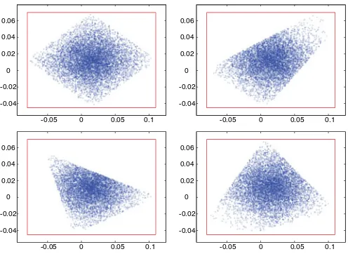
is not invertible. Thus, by choosing a specific inversion .#, an unnecessary assumption is made, and it may happen that an admissibleφproduces a negativef⊥=S⊥X#φ. Fig. 2 displays the domain reached by the center of pressure (COP): For a necessary and sufficient condition, the whole support polygon should be reached. Using the 2-norm, only the included diamond is reached, as presented in Fig. 2. Various included quadrilaterals are reached when using other norms for the inversion operator #_.

2) Using Contact Forces as Variables: The problem is that the forces fi cannot be uniquely determined fromφ, while it

is possible to determineφfromfi. To cope with this problem,

-0.04

Fig. 2. Random sampling of the reached support region. The actual support polygon is the encompassing rectangle. The point clouds display the ZMP of random forces admissible in the sense of (35). Random forcesφare shot, and the correspondingf=X#φare computed. Ifφrespects (35), the corresponding COP is drawn. Each subfigure displays the admissible forces for a different weighted inversion (the Euclidean norm is used on the top left, and random norms for the three others). Only a subregion of the support polygon can be reached, experimentally illustrating the fact that (35) is a too-restrictive sufficient condition.

written with respect to the variables u= (τ,q, φ, f)¨ , with the HQP (30)_≺(22)_≺(31)_≺(32)_≺(14).

Compared with the HQP formulated at the end of Section IV-B, this new formulation considerably reduces the size ofJc, and,

thus, the whole complexity of the resolution scheme. Addingφ

inside the variables acts as a proxy on the bigger dimension variable f. The contact forces only appear for the positivity condition (32) and in the relation with φ (31). The HQP is now sparse on the column corresponding tof, which could be optimally exploited only if the solver is sparse. In the following, we rather propose reducing the formulation, while making the constraint matrix dense.

3) Reducing the Size of the Variablef: It is possible to de-couple in (31) the relation betweenφand the tangent compo-nents off.φwas previously expressed at an arbitrary pointcof the contact body (φ=cφ). Consider the pointochosen at the interface of contact (e.g.,ois the projection ofcon the contact surface).oφdenotes the 6-D forces ato, which is expressed in terms ofoφas follows:

witho_{xbeing the coordinates of any quantityxin the frameF} o

centered at o, having its z-axis normal to the contact surface. From (31) and (36), it comes

o_fx₌

expression reveals a decoupling inc_{φ. The forces}o_fx,y _{and the}

torqueo_τz _{are expressed in terms off}x,y

are unconstrained and can be removed along with the associated constraints (37.1), (37.2), and (37.6). The reduced rigid-contact constraint can be expressed as follows:

Qc

B. Generalization to Multiple Contacts

Equation (30) considers one single body in contact. If several bodies are in contact or one body is in contact with several planes, a forceφiis introduced for each couple plane body in

contact

A¨q+b+

i

J_i⊤φi=STτ. (39)

For each body in contact, the same reasoning can be applied separately. Support polygons and normal forcesf_i⊥have to be introduced. For each contact,f_i⊥ is constrained to be positive and can be mapped toφiusing (36). The zero-motion constraint

corresponding to contactiis denoted by (22.i) and the positivity constraint by (38.i), whereirefers to the index.

C. Multiple Tasks and Final Norm

Similarly, for several tasks, (14.j) denotes the constraint for each taskj(using the same notation wherejrefers to the index). After adding all the tasks, some DOF may remain unconstrained. In that case, it is desirable to comply with Gauss’ principle. This is possible by imposingq¨=a0as the least priority, wherea0is the acceleration of the unconstrained system.8_{This has strictly} the same effect as weighting all the pseudoinverses byA−1_{, as} done in (17) [56]. However, no damping mechanism acts in the corresponding DOF that would reduce the motion energy and stabilize the system. The task-function formalism requires the

system to be fully constrained to ensure its stability in terms of automatic control (Lyapunov stability, [13]). On a physical robot, damping is always present. For perfect systems like sim-ulations, where damping is absent or is perfectly compensated, it is better to introduce, at the very last level, a task to cope with the case of an insufficient number of tasks and constraints to fulfill the full-rank condition

¨

q=−Kq.˙ (40)

Various full-rank constraints could have been considered (min-imum acceleration, distance to a reference posture, etc.). The choice of using the minimum velocity constraint is arbitrary.

Finally, the complete HQP forncontacts andktasks is written as (39)_≺(22.1) _≺(38.1) _{≺ · · · ≺}(22.n)_≺(38.n)_≺(14.1)

≺ · · · ≺ (14.k) _≺ (40), with the optimization variables u=

(τ,q, φ¨ 1, f1⊥, . . . , φn, fn⊥).

D. Opening to Other Classes of Contacts

The model (22)–(38) is built on the rigid point contact. From the basic point model, many other variations can be built. In particular, it is straightforward to obtain edge contact. Elastic contact can be defined by modifying the equation of motion (22) [41]. Linearized friction cones can also be considered, by replacingJ_c⊤f withJ_c⊤Gλ_andf⊥_{≥0 with}λ_{≥0, whereG}

is a family of generators of the linearized cone, andλ_{are the}

multipliers of these generators [38], [39]. Motions with slips are made possible by removing the motion constraint (22) in the tangent directions, and setting a constraint on the tangent force to be outside the friction cone.

However, the limitation in the viewpoint of real-time control is the size of the obtained QP formulation. Typically, a good cone approximation is obtained with 12 generators, which introduce 12 new variables per point of contact. The prospectives of this study for humanoid robot control are to find reduced formula-tions to handle these situaformula-tions. In the remainder of this paper, the reduced rigid planar formulation is used, since it maintains a relatively low computational cost, while covering many possible situations with the humanoid robot.

VI. CONTROLLAWROBUSTNESS

A. Comparison of (38) With the Zero-Moment Point Condition

A classical situation is to have one or two feet of the hu-manoid robot in contact with a flat horizontal floor. In this case, a classical condition to enforce the contact stability is to check that the ZMP stays inside the support polygon [63], [64]. In this section, this condition is proved to be equivalent to (32).

Proposition VI.1: In the case of contact with a horizontal floor, the rigid-contact condition (32) is equivalent to the well-known contact stability condition, which requires that the ZMP belongs to the support polygon.

1) Sufficient Implication: As earlier, the robot is supposed to be in single support.9_{The contact surface is supposed to be} horizontal. The ZMP (also called COP [65]) can be defined as

9_{The same reasoning holds with several bodies in contact with the same} horizontal plane.

the barycenter of the contact points pi delimiting the contact

surface of the foot with a horizontal floor, weighted by the normal componentf_i⊥of the contact forcesfiat these points10.

z= 1 Σifi⊥

Σipifi⊥. (41)

In affine geometry, it is well known that the convex hull of a polygon can be written as the set of all positive-weight barycen-ters of the vertices [66]. The rigid-contact condition defined by (32) ensures that each f_i⊥ is positive. Consequently, (32) to-gether with (41) ensures that the ZMP belongs to the convex hull of the contact pointspiwhich, by definition, is equal to the

support polygon.

2) Necessary Implication: On the other hand, if the ZMP belongs to the support polygon, there always exists a distribution of contact forcesfiat the pointspi, having positive components

f_i⊥, and such that the ZMP is the barycenter of thepiweighted

by thef⊥

i . This is sometimes referred to asweak contactstability

[62] for which the ZMP is known to be a reduced condition [67]. When the support polygon is defined by more than three contact points (l >3), an infinite number of possible barycenter weights

f⊥

i can be found to define the ZMP. For given weights, one of

thef⊥

i can be negative (this is typically what happens in Fig. 2).

However, since the ZMP is inside the convex hull, there is at least one combination of nonnegative weights that reaches it.

B. Brief Stability Analysis

The inverse dynamics schemes are known to be sensitive to modeling errors [68]. In particular, if the inertia parameters are not perfectly known, the application of the reference torques will lead to different accelerations. The estimated value ofX

is denoted by X. The solution of the QP is equivalent to the solution given by the pseudoinverse if none of the positive-force constraints are active otherwise, it has a similar form with an additional projection and can be written for one task

τ= (JA−1PfST)+(¨e∗+μ) (42)

wherePfis the projection operator onto the contact zero-motion

constraint (22) and onto the set of contact positive-force con-straints (38) that are active. Using (26), the observed task accel-eration when applying this control law, which is also denoted byˆ., is

e¨=JA−1PcST(JA−1PfST)+(¨e∗+μ)−μ. (43)

Since PcPf =Pf,e¨= ¨e∗ if all the estimations are perfect.

If the estimations are biased, applying the control (42) in closed loop at the whole-body level is known to keep the stability properties of the control law ¨e∗ in the task space iff JA−1_P

cST(JA−1PfST)+ is definite positive [13]. When the

estimation error is due to an inaccurate dynamic model, a clas-sical solution to reduce the estimation error is to rely on a time-delay estimation, i.e., reporting the biases observed at one iteration of the control on the next iteration [69]. However, this

technique cannot perfectly cancel the errors of estimation; thus, (43) still holds.

The reference¨e∗ is not perfectly tracked. It is also true for the contact forces computed by the solver. Indeed, the observed forces are

ˆ

φ= (Jc⊤)#AJˆc⊤φ∗+ (JcA−1Jc⊤)−1JcA−1Aq¨∗ (44)

whereφ∗_andq¨∗ _{are the reference force and acceleration}

com-puted by the HQP, andJ˙cq˙ is neglected. The second term is

close to 0 whenAis not too far fromA. Similarly, the first term is nearly the identity matrix when the estimation is correct. The previous equation can be summarized by

ˆ

φ= (I+ǫ1)φ∗+ǫ2q¨∗ (45)

withǫ1 andǫ2 being two matrices that tend to zero when the estimation tends to perfection. When the ǫi are not null, the

observed forceφˆis biased with respect to the solver predictions. If the bias is too great, there is no guarantee that the observed forceφˆwill maintain the contact; then, the property of stability can be lost.

In conclusion, applying the computed torques in closed loop ensures the stability of the control as long as the observed forces respect the contact positivity-force constraint.

C. Contact Condition as a Qualitative Robustness Indicator

The previous stability analysis is not very instructive in prac-tice, since it is barely possible to predict when the observed

ˆ

φwill keep the contact stability. The robustness of the control scheme thus relies on the behavior ofφˆ. It is interesting to pro-vide an indicator of how easy it is forφˆto leave the acceptable domain. When considering one single point in contact as in Sec-tion IV, this indicator is straightforward to choose. Consider the normal force valuef⊥∗computed by the solver. Iff⊥∗is large, then for smallǫ1, ǫ2, we can be very confident thatfˆ⊥will be positive and keep the contact stable. Then, for one single contact point, the positivity off⊥∗_{is a good indicator of the robustness}

of the control.

For more than one single contact point, it is not possible to use a direct combination of the normal forces as an indicator. Indeed, there is an infinite number of possible force values, all of them being equivalent in terms of the robot behavior. Once more, this is connected to the results displayed in Fig. 2. The computed solution may include one zero normal force, while another solution exists with strictly positive values. When considering a single planar contact, the ZMP is a good indicator of robustness: when the predicted ZMP z∗ is far inside the support polygon, then we can be very confident that the observed ZMPzˆwill stay inside the support polygon, which means in return that all thefˆ⊥_{are positive.}

If the contacts are not coplanar, the ZMP is not defined. In that case, the generalized zero-moment point (GZMP) [70] has been proposed. Contrary to the ZMP or to (38), the GZMP is not a constructive criterion, i.e., it has not been used to generate a motion or a control law. The idea of the GZMP is to find from the 3-D contact points a plane that will act like the floor plane for the ZMP. On this plane, all the force boundaries are

projected, defining a 2-D polygon. The GZMP exists in this same plane. The contact-stability criterion says that the GZMP should remain inside the 2-D polygon. The GZMP is easy to display. It is easy to visualize the distance to the boundaries and thus to have a qualitative evaluation of the motion robustness with respect to the contact stability. The GZMP needs some implementation work in order to be calculated, since the 2-D projection plane is deduced from geometrical computations. Moreover, it is only an approximated criterion, since the friction forces are neglected. To cope with these limitations and obtain a generative criterion, the GZMP was augmented in [67]. However, this last criterion, like (38), cannot be easily plotted, and is thus not relevant to judge the robustness of the obtained motion.

Consider the six first rows of the dynamic equation. The dependence onτdisappears

¯

A¨q+ ¯b= ¯Jcf (46)

where A¯,¯b, andJ¯c are the first six rows of, respectively, A,

b, and JcT. For a given q¨∗, the left term is constant, which

is denoted byψ∗_{. It corresponds to the actuation of the}

free-floating body that cannot be accomplished by the motors. The variablef can be partitioned in two partsf = (f♥, f♠):f♥is

unconstrained, whilef_♠ is subject to the positivity constraint.

¯

Jcis similarly partitioned intoJ¯♥andJ¯♠. The setK♠:={ψ= ¯

J_♠f, f >0}is a 6-D cone that can be expressed by its facets. The motion is robust to the parameter error if the pointψ∗−

¯

J_♥f_♥= (I−J¯_♥J¯_♥+)ψ∗ _{is deep inside the cone. The distance}

from this point to the closest facet ofK_♠ can be used as a measure of the robustness of the motion. The scaling between torques and forces is done using a characteristic length of the system (1 m for a human-size robot). In the following, this criterion is referred to as robustness criterion.

VII. EXPERIMENTS

Three sets of experiments are presented in this section. The first one presents a simple oscillatory motion that illustrates the saturation of the contact-stability constraints. The second one presents a complex sequence of tasks to make the robot sit in an armchair using several successive contacts. This motion is also executed by the real robot. The last experiment presents a dynamic transition of contacts. First, the setup is detailed.

A. Experimental Setup

The inverse formulation of the dynamic equation of motion (30) is given to the HQP solver. However, since it computes explicitly bothτandq¨, it solves simultaneously the forward and inverse dynamics of the robot. Both values can then be used as control input. The accelerationq¨can be integrated in simu-lation, or provided as control input to the robot servo control; or the torques can be given as the robot control, or provided to a dynamics simulator. On current humanoid robots, such as HRP-2, only the first solution is possible.11 _{However, this} so-lution has the drawback that the servo will be on the position

variables, while as explained in the previous section, the ro-bustness mainly relies on the accuracy of the force variables. In simulation, both solutions are possible. The second solution is more beneficial, since it makes it possible to double check the dynamic computations.

In practice, we have used this last solution. The dynamic sim-ulator AMELIF [73] was used to resolve the forward dynamics from the computed torquesτ∗_{. The simulator checks the}

colli-sion, computes the acceleration from the collision set and the torque input using a linear solver, and numerically integratesq¨

using a classical Runge–Kutta of the fourth order. The current set of contacts is then provided to the control solver, along with the current position and velocity of the robot. The control is updated every 1 ms. It is computed using the control frame-work SOT [34] and the dedicated solver [27]. The result of this simulation is a joint trajectory of the robot, which complies to the multibody dynamics. This trajectory is replayed on the real robot using a position-control mode.

The task set used in the three presented motions is the fol-lowing. A first task function is used to control the position and orientation of one operational point of the robot (e.g., grippers, head, chest). The task error is the positionpand angle-vector orientationrθ [74] of the operational point with respect to a referencep∗_,rθ∗_{expressed in the world frame}

eop =

_p−p∗

rθ⊖uθ∗

. (47)

The reference acceleration is computed from this error as a proportional-derivative control law

¨

e⋆_op =−λ_peop−λ_{de˙op (48)}

wheree˙op =Jopq˙is the velocity in the task space and the gains λ_{p and}λ_{d are used to tune the convergence velocity (usually,} λ_{d = 2}λ_{p). For tracking a moving target, a fixed high gain is}

used forλ_{p. When reaching a fixed target, an adaptive gain is}

typically used

λ_{p :e →(}λ₀₋λ_∞)e−βe₊λ_{∞ (49)}

whereλ_{0 is the gain when the error is null,}λ_{∞ is the gain far}

from the target, andβadjusts the switching behavior between the gains. A typical setting is(λ_0,λ_{∞, β) = (450,15,100). A}

second taskegazeis used to servo the projectionsof one point of the environment on the right camera plane to a reference positions∗[14]

egaze=s−s∗. (50)

The reference acceleration¨e∗is also defined by (48). The torque magnitude is also bounded. Since the torques are included in the vector of optimization variables, it is trivial to express the torque limits by a simple bound on these variables

τ_≤τ_≤τ (51)

withτ =−τbeing the maximum torque value.

Similarly, bounds have to be set on the joint positions. Since the positions are not variables of the solver, the constraint is set

on the joint accelerations

q≤q+TSq˙+

TS2

2 q¨≤q (52)

whereqandqdenote the lower and upper joint limits, respec-tively, andTS is the length of the preview windows. In theory,

the control sampling time∆T =1 ms should be used forTS.

In practice, a smoother behavior can be obtained by adjusting this valueTS := ∆λ_sT whereλs can be tuned as the gain of the task. We usedλ_{s=0.1 to generate the following motions.}

B. Experiment A: Swing Posture

1) Description: The objective of this experiment is to vali-date the contact stability constraint. It is inspired by a biome-chanics experiment, which aims to test the human swinging posture behavior with respect to the same constraints [75]. A tracking task is imposed upon the robot head to make it os-cillate. Depending on the frequency and the amplitude of the oscillation, forces are obtained at the contact points, which may saturate the contact constraint. The taskehead, which is given by (47), is imposed upon the head operational point, where only the translation on the forward axis is selected. The reference posi-tion is given by a time-varying sinusoid, around a central point

xc=0.02 and with amplitude of 5 cm and frequency 0.3 Hz

(low frequency), 0.56 Hz (medium frequency), or 0.9 Hz (high frequency). The gain is set toλ_{p :=}250 to ensure good tracking. The complete SOT is (39)_≺(22)_≺(38)_≺(51)_≺(52)_≺ehead

≺(40).

In theory, the contact points are defined from the 3-D model of the robot. However, in practice, we never consider the real support polygon, but a smaller one. This simple trick ensures increased robustness of the motion when trying to replay it on the robot. For example, on the feet, the support polygon is often defined as a square of 4 cm centered below the ankle axis [76], [77]. The obtained robustness can be evaluated afterward with respect to the real support polygon.

The motion is played four times. In the first two executions, both feet are flat on the ground and the reference is oscillating at low and medium frequencies, respectively. For the next two executions, the right gripper contact is added, and the motion is played at medium and high frequencies. In the following, the four motions are referred to as 2pt-low,2pt-medium, 3pt-medium, and3pt-high, respectively.

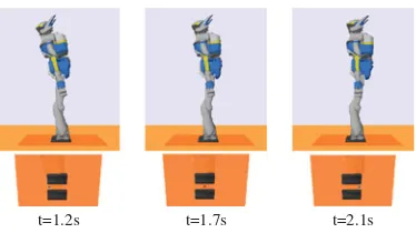
2) Results: The experiment is summed up by Figs. 3–6. The motion is displayed in Fig. 3. The robot is oscillating forward and backward to follow the head reference. The two motions

2pt-lowand2pt-mediumwere already detailed in [1] where the plots of joint positions and torques can be found. When only the feet are contacting, the stability of the motion can be evaluated by displaying the ZMP, plotted in Fig. 4. At low frequency, the ZMP does not saturate because the demanded accelerations are small enough. At medium frequency, the accelerations are larger and the ZMP saturates. Since the real support polygon is about 20 cm wide, there is a large offset that ensures a good robustness when executing this motion on the real robot.

t=1.2s t=1.7s t=2.1s

Fig. 3. Experiment A. (Top) Snapshots of the oscillatory movement 2pt-medium. (Bottom) Feet and ZMP positions at the corresponding instants. The ZMP saturates on the front when the robot is reaching its top amplitude and decelerates to go backward. Similarly, the ZMP saturates on the back.

0.5 1 1.5 2 2.5 3 3.5 4 −0.02

−0.01 0 0.01 0.02

ZMP x−position (m)

low frequency medium frequency ZMP limit

Fig. 4. Experiment A. ZMP position along the forward (x) axis for the two motions with only the feet contacts. The support polygon is a 4-cm-wide square centered on the ankle joint. The ZMP does not saturate when the motion oscil-lates at low frequency. It saturates at medium frequency.

0 0.5 1 1.5 2 2.5 3 0

5 10 15 20 25 30 35 40 45

Distance to cone

low 2pt solver low 2pt real medium 2pt solver medium 2pt real 3pt medium 3pt high

Fig. 5. Experiment A: Robustness criterion (see Section VI-C). For the first two motions2pt-lowand 2pt-medium, the criterion is given with respect to the support polygon defined in the solver (small contact surface) in bold, and with respect to the real support polygon taking into account the friction cone (linearized by twelve facets) in nonbold. This criterion behaves similarly to the distance of the ZMP to the support polygon. The criterion is plotted for 3pt-mediumand3pt-high. If the solver support polygons are considered, the distance is infinite. It is only plotted for the distance to the friction cone.

0.5 1 1.5 2 2.5 3 8.5

9 9.5 10 10.5

time (s)

Computation time (ms)

low 2pt med 2pt med 3pt high 3pt

Fig. 6. Experiment A: Computation time. For the motion2pt-medium, the saturation of the force constraints clearly induces an increase of the compu-tation cost, whereas for2pt-low, the cost remains constant. For3pt-medium, the cost is constant (no saturation) but higher in average due to the additional contact. Finally, the cost of3pt-highis higher and varies when the constraints are saturated.

projected into the space of the spatial forces expressed at the waist point. Then, the distance of the pointψ∗(46) to this con-straint set is computed. The result is plotted in Fig. 5. First, the distance is computed to the constraint set of the solver (the 4-cm-wide support polygon). As expected, the distance is null when the ZMP saturates. More interestingly, the distance can be com-puted to the real constraints by taking into account the true poly-gon as well as the linearized friction cones at the contact points. The friction coefficient was set toK=0.5. In that case, the robustness criterion is always strictly positive, showing that the motion is robust to small perturbations or model uncertainties.

Using only the feet as contacts, it is not possible to follow the reference at high velocity. A third contact point is added to increase the stability domain. The contact polygon is a square of 5 cm centered at the gripper terminal point. Contrary to the ZMP, the robustness criterion (see Section VI-C) is still valid with noncoplanar contacts. When the friction cones are not con-sidered (slidingless contact), it is always possible to find a set of contact forces following a given center of mass (COM) ac-celeration (the system is said to be inforce closure[78]). In that case, the distance to the constraint set is always infinite. The robustness criterion is finite when the friction cones are consid-ered. The friction coefficient at the gripper is set toK=0.1. At medium frequency, the motion can be considered very robust since the criterion is always very far from 0. If the frequency is increasing, the criterion remains smaller. It then jumps from one constraint edge to another, which explains the discontinuities. The computation time depends on the number of contacts, tasks, and active constraints, as shown in Fig. 6.

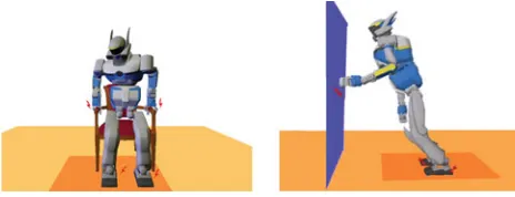
C. Experiment B: Sitting in the Armchair

1) Description: The second experiment illustrates the possi-bilities of multiple noncoplanar contacts during a more complex sequence of motion. The robot sits in an armchair (see Fig. 7). First, contacts of the left then right grippers are found with the armrests to increase the contact stability domain. Then, the pelvis is brought in contact with the seat.

At the highest priority of the stack, the limits (51) and (52) ensure that the joints and actuator limits are respected. Two taskser h andelh, which are defined by (47), are set on each

s 9 1 = t s

5 1 = t s

7 = t s

0 = t

Fig. 7. Experiment B: Snapshots of the motion executed on the real HRP-2 robot. The robot is standing on both feet (t=0 s). It first looks left and grasps the left armrestt=7 s. It then looks right, grasps the right armrest (t=15 s), and, finally, sits (t=19 s).

0 5 10 15 20 25

rh e lh e gaze e waist e

time (s)

pre−grasp grasp contact pre−grasp grasp contact

left center right center down

Fig. 8. Experiment B: Sequence of tasks and contacts. The gaze task focuses sequentially on the left and right armrests and on a virtual point in front of the robot. The pregrasp tasks are set at the vertical 10 cm above the grasp position.

0 5 10 15 20 25

0 0.1 0.2 0.3 0.4 0.5 0.6 0.7 0.8 0.9 1

time (s)

Normalized joint position

R.hip R.ankle L.hip L.ankle Pan.chest Tilt.chest Pan.neck

Fig. 9. Experiment B: Normalized joint position (0 and 1 are, respectively, the lower and upper limits) of the right and left hip and ankle, chest, and neck joints. The joint limits are properly avoided. When a limit is reached, one or several joints move in reaction to overcome the saturation.

0 5 10 15 20 25

0 50 100 150 200 250 300 350 400

time (s)

Normal forces (N)

L.foot R.foot L.grip R.grip

Fig. 10. Experiment B: Vertical forces distribution.

−0.25

−0.2

−0.15

−0.1

−0.05

0

0.05

0.1

0.15

0.2

−0.1 −0.05 0 0.05 0.1 0.15 0.2 0.25 0.3 0.35 0.4

com x coordinate (m)

com y coordinate (m)

Left Foot Right Foot

First part Second part Third part

Fig. 11. Experiment B: Position of COM. The three phases correspond to changes in the number of contacts (first the two feet, then the left gripper, and, finally, both feet and grippers). First, the COM stays forward, but is, finally, moved backward to reach the second armrest and move the pelvis down to the seat.

0 5 10 15 20 25

0 5 10 15

time (s)

Distance to the cone

Fig. 12. Experiment B: Robustness criterion (see Section VI-C). The distance is computed with respect to the friction cones. The friction coefficient at the armrests is roughly estimated to be five times less than at the sole. The less robust part occurs during the final phase, where the waist moves down.

0 5 10 15 20 25

18 20 22 24 26 28

time (s)

Computation time (ms)

right handle; finally, using both handle supports, it moves the pelvis down to sit.

2) Results: The experiment is summarized in Figs. 7–13. The key frames of the motion executed by the robot are given in Fig. 7. The sequence of tasks is summarized in Fig. 8. On each of the following figures, the chronological sequence is recalled by vertical stems at the transition instants. During the motion, the joint range is extensively used. The most representative joint trajectories are plotted in Fig. 9. The neck joint reaches its limit while looking left. In reaction, all the other aligned joints move to overrun the neck limitation (chest joint of course, but also hip and ankle joints). The right hip then reaches its limit. In consequence, all the motions of both legs are stopped, due to a lack of DOF to compensate this limit. The chest joint absorbs all the subsequent overrun to fulfill the task. Again, the neck joint reaches its limit when looking right. This time, the velocity of the joint when it reaches its limit is higher, which leads to a strong acceleration of the chest, and consequently brings the neck out of its limit. This behavior could be damped if necessary by tuningλ_{sin (52). The chest joint, finally, reaches its limit at the}

end of the right-grasp task, which produces a limited overrun on the other joints. All the joints are properly stopped at the limit, and can leave the neighborhood of the limit without being stuck, as it may appear with some avoidance techniques.

The contact with the two armrests is very useful to control the descent of the waist. The vertical forces on each support are plotted in Fig. 10. In the beginning, the weight is fully supported by the two feet, as shown in Fig. 11. Aftert=8 s, the left arm is used to sustain the robot. However, the robot upper body is still in front of the chair, and this contact is not fully used yet. In order to reach the second armrest, the robot has to move its weight back (see Fig. 11) and use the left-arm contact to ensure its balance: nearly half of the weight is then supported by the arm. Finally, the right armrest is grasped, and the robot distributes its weight on the four contacts equally.

Neither the COM nor the ZMP can give a proper estimation of the stability, since the motion is neither quasi-static nor sup-ported by planar contacts. The robustness estimator presented in Section VI-C is plotted in Fig. 12 with respect to the linearized friction cones at both feet and grippers. The motion is very stable, except at the end of the motion, when the waist moves down. At that time, the robot is using the tangent forces of the grippers on the armrest, which nearly saturates the friction cone. In consequence, this part of the motion is less robust when exe-cuted by the real robot. Indeed, since the armrests do not respect the hypothesis of rigid contact and due to this lack of robustness, it can be observed that the toes nearly leave the ground during this phase of the motion. This effect is very interesting, since it confirms the relevance of the robustness criterion. Of course, this undesirable effect could be avoided by setting a more ac-curate model of the environment or adding a safety limit to the positivity constraint in the solver.

Finally, the computation times are plotted in Fig. 13. The SOT is nearly full. In that case, the computation cost is around 20 ms per iteration, i.e., five times the real time if controlling the robot at 200 Hz. The computation cost depends on the number of tasks and even more on the number of contacts, as shown by the computation increase att=8 s andt=18 s.

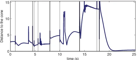
D. Experiment C: Dynamic Contact Transition

1) Description: At the beginning of the motion, the robot is standing on both feet and its COM is artificially pushed forward using a task on its chest. The robot is then out of its domain of quasi-static stability. The only solution to restore the balance is to change the set of supports. The two grippers (first the left, then the right) are then sent forward to establish a contact with the wall, in order to increase the set of support contacts and to restore the balance. An overview of the motion is given in Fig. 14. Three tasks of type (47) are used: one task on the chest, which controls only the translation; another one on each gripper controls both the translation and the rotation. The COM is not explicitly controlled. The sequence of tasks and contacts is given in Fig. 15.

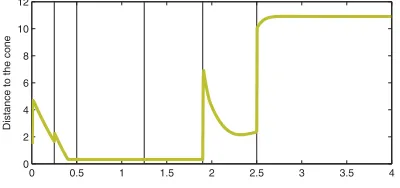
2) Results: The experiment is summarized in Figs. 14–18. If using only quasi-static movements (i.e., reaching while keeping the COM inside the feet support polygon), the maximal reaching distance of HRP-2 is around 85 cm. In this motion, the wall is positioned 1 m in front of the robot, as shown in Fig. 14. The motions of the COM along with the forward direction are plotted in Fig. 16. The COM quickly leaves the support polygon in the beginning of the motion, due to the artificial motion of the chest. Fromt=0.7 s, the COM is out of the support polygon with a positive velocity. It is then impossible to bring it back to stability without changing the supports. The balance is restored aftert=2.5 s, with the COM coming back to zero velocity. The stability is evaluated using the robustness criterion presented in Section VI-C. When only the feet are in contact, the ZMP is at the forward limit of the support polygon, which corresponds to a low robustness. The robustness increases when the first gripper enters into contact. However, at that time, the tangent forces of the gripper on the wall are high. The robot can then lose its balance by rotating on one of the gripper–foot edges, as already observed in [70]. The second gripper helps us to improve the stability by decreasing the tangent forces at each contact point. The vertical forces are plotted in Fig. 18. On the grippers, the vertical direction corresponds to the tangent to the contact. Betweent=1.9 s andt=2.5 s, the tangent forces at the left gripper are high, at the limit of the friction cones, which corresponds to a weaker robustness of the motion (the gripper is close to slide).

VIII. CONCLUSION