Model Development of Children Under Mortality Rate With Group Method of Data Handling

(1)

Model Development of Children Under Mortality Rate With Group

Method of Data Handling

I. Lukman

#1

, M. N. Hassan*

2

, Noor Akma I

#3

and M. N. Sulaiman

#4 #1_{Department of ManagementFaculty of Economics}

Universitas Malahayati BandarlampungIndonesia

Ilukman371@gmail.com

*2_{World Health OrganizationCambodia Chapter, Pnom Phen}

3_{Institute for Mathematical Reseach/Department of MathematicsUniversiti Putra Malaysia}

#4_{Department of Computer ScienceFaculty of Computer Science}

and Information TechnologyUniversiti Putra Malaysia Serdang D. E. 43400 Selangor

(Received Mei 2012, Accepted August 2012)

Abstract—in this research we examine aspects of the interdependence between economic development and the use of environmental and natural resources assets from global data published by united nations. for that purpose, we use data mining techniques.data mining techniques applied in this paper were: 1) group method of data handling (gmdh), originally from engineering, introducing principles of evolution - inheritance, mutation and selection - for generating a network structure systematically to develop the automatic model, synthesis, and its validation; 2) step wise regression were also applied for some cases.data sets for this research consist of one sets integration data of air quality data and macroeconomic data of the cross-country data of world development indicator 2003 (wdi 2003). the result shows that the mortality rate of children under five years old is dependent on sanitation and water facilities obtained from gmdh results. however, the results from step-wise regression shows that mortality rate was dependent on annual deforestation, particulate matter, nationally protected area, with the big contribution was from annual deforestation.

Keywords— data mining, world development indicator, gmdh, deforestation, underfive years old mortality rate.

I. INTRODUCTION

In recent years a great deal of effort has been invested in documenting, measuring and valuing environmental trends in Asian countries. The data indicated that growth rates of energy demand, industrial emissions, and the depletion and degradation of many forms of environmental services and natural resources have matched or even exceeded rates of economic growth [4]. Even in the regions and countries with the brightest records, it seems that high rates of growth and poverty alleviation have apparently come at considerable environmental cost [4].

Air quality is a major problem affecting citizens in both developed and developing countries. Good air quality management underlie increased economic and social welfare in many developing countries in terms of Gross Domestic Product (GDP) growth, and decreasing social costs due to the illness caused by bad air quality.

Recent estimates of the increase in daily mortality showed that on a global scale 4-8% of premature deaths are due to exposure to particulate matter in the ambient and indoor environment [17]. Moreover, around 20-30% of all respiratory diseases appear to be due to ambient and indoor air pollution, with emphasis on the latter [17].

Research conducted on environmental economics have always touch on the link between economic and environment. The Kuznets curve so far has been an important topic for that matter. The environmental Kuznets curve (EKC) theory suggests that economic growth in the long run may reduce environmental problems [3]. A survey of the EKC literature reveals that the relationship between income and environmental quality also varies according to the type of pollution involved ([3]). Also a Norwegian time series research showed that total emissions of lead, SO2 and CO have

decreased significantly as income increased over the last decades [3].

(2)

©Universitas Bandar Lampung 2013

growth, and it might be the other way around [3]. The analytical literature on growth and the environment in Asia tends to agree that environmental damage is costly to regional economies, and the economic growth and environmental damage are associated, but the relationship is neither linear nor even monotonic, and it was clearly seen in the diverse experiences of tropical Asian economies over recent decades that the nature of the growth-environment link depends on the changing composition of production and on growth-related changes in techniques and environmental policies [4].

II. METHODOLOGY

General Experimental Methods

The database or data sets for this research comprised of an integration between air quality data and macroeconomic data. These data were obtained from cross-country data of The Little Green Data Book 2003 of

World Development Indicator 2003

(http://www.worldbank.org/data). The variables of air quality data are CO2 emissions per unit GDP, CO2 per

capita, consumption of chlorofluorocarbons (CFCs), Particulate Matter (PM), damage caused by CO2, damage

caused by PM. The variables of macroeconomics and the national assets are population, Gross Domestic Product (GDP), Gross National Income (GNI), urban population, land index, population density, forest area, forest area in percentage, annual deforestation, mammal species total known, mammal species threatened, bird species total, bird species threatened, nationally protected area, GDP per unit of energy use, commercial energy use per capita, share of electricity generated by coal, passengers cars, freshwater resources per capita, freshwater withdrawal total, freshwater withdrawal in agriculture, access to an improve water source, access to an improve water in rural, access to an improve water in urban, access to sanitation, access to sanitation for rural, access to sanitation for urban, under five years old children mortality rate, consumption of fixed capital, education expenditure, energy depletion, mineral depletion, net forest depletion, and adjusted net saving.

Data mining application in the economic evaluation of air pollution is relatively new especially on the analysis of integrated data between the economic variables and air pollution variables. Data mining algorithms of Group Method of Data Handling (GMDH), was utilised in the analysis.

Data Selection

Initially five data sets were considered. They were 1) World Development Indicator (WDI) 2003 from the World Bank (http://www.worldbank.org.data), 2) Economic Growth and Environmental Quality Data from Shafik and Bandyopadhyay of World Development Report 1992 (http://www.worldbank.org.data), 3) Indonesian air quality data from Minister of Environmental Office, Jakarta along with macroeconomic

data from Biro PusatStatistik Indonesia, 4) Malaysian Air Quality Data from ASMA (AlamSekitar Malaysia SdnBhd), Malaysia, and 5) Environmental Economic data from Nationmaster.com. In this data selection, out of five data sets only one set was chosen, namely environmental economic data of WDI 2003. The data sets from Indonesia, Malaysia, and Shafik and Bandyopadhyay (1992) were not selected due to excessive in missing values. The Indonesian data were not selected due to mismatch between air quality years and the macroeconomic years. The Malaysian air quality data were not selected because the macroeconomic data were not available.

The data sets of WDI 2003 comprised of 208 countries (cases) by 47 variables are arranged as follows: three cases were deleted due to severe incomplete data; therefore only 205 out of 208 cases were used. Thus, there were 9635 cells. These 205 cases were still having missing values, which then imputed by EM algorithm and hot deck imputation.

EM Algorithm for Data with Missing Values

The EM algorithm [5] is a technique that finds maximum likelihood estimates in parametric models for incomplete data. EM capitalizes on the relationship between missing data and the unknown parameters of a data model. If the missing values patterns are known, then estimating the model of parameters will be straightforward. Similarly, if the parameters of the data model are known, then it will be possible to obtain unbiased predictions for the missing values. The interdependence between model parameters and missing values suggested an iterative method where to predict the missing values at first based on the assumption of the values of parameters. Then use these predictions to update the parameter estimate, and be repeated. The sequence of parameters converges to maximum-likelihood estimates that implicitly average over the distribution of the missing values. The EM algorithm is an iterative procedure that finds the maximum likelihood estimator (MLE) of the parameter vector.

A sample covariance matrix is computed at each step of the EM algorithm. If the covariance matrix is singular, the linearly dependent variables for the observed data are excluded from the likelihood function. That is, for each observation with linear dependency among its observed variables, the dependent variables are excluded from the likelihood function. Note that this may result in an unexpected change in the likelihood between iterations prior to the final convergence [16].

Hot-Deck Imputation

(3)

obtained from different analysis are consistent with one another. The main principle of the hot-deck method is by using the current data (donors) to provide imputed values for records with missing values. The procedure involves finding the donor that matches the record with missing values. The matching process is carried out using records of certain variables. The records match if they have the same values on the records of those variables [7]. Other hot-deck techniques include distance function matching or nearest neighbor imputation in which a non-respondent is assigned to the item value of the nearest neighbor. Hot deck imputation fills in missing cells in a data matrix with the next most similar case value.

Once the hot deck imputation determines which case among the observations with complete data is the most similar to the record with incomplete data, it substitutes the most similar complete case value for the missing variable into the data matrix.

Data analysis then can proceed using the new complete database.

Data Enrichment and Coding

Additional data might be important for conducting data mining studies. Data coding phase might include processing of deleting some records (e.g., records which do not have enough meaningful information) and recording or transforming other information.

Data Mining Process

This phase is the process of knowledge discovery in databases, offering automated discovery of previously unknown patterns as well as automated prediction of trends and behaviour (pattern generation). In this phase, various modeling techniques are selected and applied, and their parameters are calibrated to optimal values. Typically, there are several techniques for the same data mining problem. Some techniques have specific requirements on the form of data. Therefore, stepping back to the data preparation phase is often needed. The techniques used in this thesis were Group Method of Data Handling (GMDH) and step-wise regression.

GMDH algorithm and step-wise regression were conducted to data from WDI 2003. The data were carefully handled due to some missing values. For WDI 2003 data, the EM algorithm and hot-deck imputation methods were imposed. The EM algorithm was conducted initially to replace the empty cells of missing values, and then the hot-deck imputation was conducted to correct the erroneous imputation by EM algorithms. This erroneous imputation was in the form of out of range values (outliers). The hot-deck imputation will replace the outliers with the nearest neighbour values.

Data set were subdivided into three subsets. The reason of subdivided into the same number between training set and testing set data is in accordance with the fundamental

steps used in self-organization modeling of inductive algorithms to split the data of N observation into training set NA and testing set NB provided that N=NA+NB (Madala and Ivakhnenko, 1994). According to Hild (1998), the subdivision of the training set or testing set was for the purpose of cross validation. Actually, the n-fold cross validation is suitable for classification only, such as to rank or to select the attribute [8] and not verify the equation model. GMDH is doing all these process automatically earlier through the process between training set and testing sets, and later conducted the cross validation process. Thus, the best models found by GMDH, it had already been passing through the n-fold validation process even though before evaluating it on validation data.

(4)

TABLE 1

DATA LAY-OUT OF WORLD DEVELOPMENT INDICATOR 2003

Table 1 is the data lay-out of WDI 2003 consisting of 47 variables and 205 cases (countries). To apply GMDH algorithm, the data were subdivided into three sub-sample sets that is the training data sets, testing data sets, and validation data sets. In the original Ivakhnenko, data sets were subdivided only to training and testing/checking, but his son G. A. Ivakhnenko (personal communications, 2004) introduced the validation data set to validate the models obtained. Abdel-Aal (2005) has also administered this validation procedure. Larose (2005) has also suggested this validation.

Results Interpretation and Validation

After the discovery phase, various graphs were presented to evaluate the predictive accuracy of the models with respect to other data sets. In this thesis the models resulted from GMDH were evaluated using the sub-sample of validation data to see the validity of the models obtained.

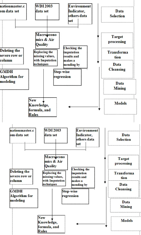
Fig. 1 shows the procedures of data mining process framework used in this paper from the data selection until new knowledge, formulas, obtained. Target data preprocessing were macroeconomics and air quality variables. In the preprocessing, transformation will take place whereby data will be cleansed which involves editing and imputation data. This then will enable the appropriate data mining process to be exempted to gain results, through GMDH algorithms. Then interpretation and its validation were made to gain new knowledge of models or formula.

Fig. 1: Data mining process framework

Group Method of Data Handling (GMDH)

(5)

algorithms and of nonparametric algorithms using clustering or analogues were developed. The choice of an algorithm for practical use depends on the type of the problem, the level of noise variance, sufficiency of sampling, and on whether the sample contains only continuous variables.

Solving practical problems and developing theoretical questions of the GMDH produced a broad spectrum of computing algorithms, each designed for a specific application (Ivakhnenko and Stepashko, 1985; Madala and Ivakhnenko, 1994). The choice of an algorithm depends both on the accuracy and completeness of information presented in the sample of experimental data and on the type of the problem to be solved.

GMDH is a combinatorial multi-layer algorithm in which a network of layers and nodes is generated using a number of inputs from the data stream being evaluated. The GMDH was first proposed and developed by Ivakhnenko (1966). The GMDH networks has been traditionally determined using a layer by layer pruning process based on a pre-selected criterion of what constitutes the best nodes at each level. The traditional GMDH method (Farlow, 1984; Madala and Ivakhnenko, 1994) is based on an underlying assumption that the data can be modeled by using an approximation of the Volterra Series or Kolmogorov-Gabor polynomial (later considered as Ivakhnenko polynomial, Farlow, 1984) as shown in equation .

Input data might consist of independent variables, functional expressions, or finite residues. This means that the function could be either an algebraic equation or a finite difference equation, or an equation with mixed terms. The partial forms of this functions as a state or summation function is developed at each simulated unit and is activated in parallel to build up the complexity.

The Steps of the GMDH Algorithm

Given a set of data of the form shown in Fig. 2, the GMDH algorithm begins with the original m independent variables, x1,x2,…,xm, and the response variable, y. Then the data divided into 2 sub-sample, that is from first row until the nt row for the training set, and from nt+1 row until n row is for the checking set.

Fig. 2: Data Structure of Original GMDH Algorithm

At each generation, the algorithm progresses through three primary steps. If the algorithm is at generation k, then the steps are as follows:

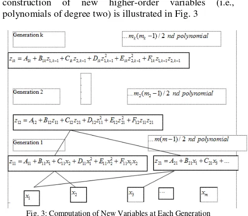
Step 1: Construction of New Variables

For each pair of independent variables, construct the second-degree polynomials of the form as follows

We assume that there are mkindependent variables that entered into generationk. The number of polynomials constructed at generation k is equivalent to the number of pairs of the mk independent variables, which is: . Thus at generation one, the algorithm generates second-degree polynomials. This construction of new higher-order variables (i.e., polynomials of degree two) is illustrated in Fig. 3

Fig. 3: Computation of New Variables at Each Generation

Step 2: Screening of Variables

At the completion of step one, the algorithm has constructed a group of new variables,

2 2

z

 

A Bx Cy



Dx



Ey



Fxy

(

1)

2

k k

m m



(

1) / 2

m m



(

1)

2

k k

(6)

. These new variables replace the old predictor variables from the previous generation in the checking set. Thus, if k=1, the variables replace the original independent variables, in the training set. Each of these new variables are evaluated for passage into the next generation by determining which variables best estimate the dependent variable, y , in the checking set. In the algorithm as proposed by Ivakhnenko (1966), the criterion used to evaluate the new variables at each generation is the root mean square, which is referred to by Ivakhnenko (1966) as the regularity criterion. The root mean square, denoted as rj, is defined as:

(3)

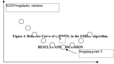
1) From (3), it showed that the regularity criterion is computed based on the values of the observations in the checking set. Also, with the use of the regulatory criterion, an arbitrary “cut-off” value,

R, is chosen such that for any , the new variable is screened out and it is not passed on to the next generation of the algorithm. In this thesis the regularity criterion is written as RMIN (regulatory criterion of minimum value).

Step 3: Test for Optimality

At the end of the second step, a value of rjis obtained for each of the variable in the kth generation. In step 3, the minimum value of these rj’sis

determined and denoted as RMINk. If RMINk is greater

than RMIN, then the algorithm stops and the polynomial (i.e., the new variable) with minimum value of the regularity criterion is chosen to be the “best” approximating model. Otherwise, RMIN=RMINk, and the

algorithm moves on to the next generation and the steps repeat. According to Farlow (1984), it has been shown that the RMIN curve has the shape as shown in Fig. 4. If the RMIN has reached S, then the developed model at that point S is the selected model. Thus, the algorithm does converge to a minimum value of the stopping criterion.

At the end of the GMDH algorithm, the final predicted values of the original response variable, y, are stored in the matrix Z. To determine the estimated coefficients in the higher-order polynomial, of the form shown in (1), the algorithm is backtracked, and the second-order polynomials from each iteration are evaluated until a

polynomial in the original variable is obtained.

The target variable for GMDH algorithm from WDI 2003 was variable of under 5 years old mortality rate, and CO2 emission per capita. The reason for taking the under

5 years old mortality as target variable from WDI 2003 due to the fact that only this variable gives the appropriate model (R2_{=0.549) when GMDH was fitted to that data.}

Under 5 Years Old Mortality Rate Model Development

The goal function was x38 or under 5 year mortality rate.

The number of countries involved 205, thus we have 205 observations to be considered. These 205 observations were divided into three parts: the training data, the testing data, and the validation data. For the training data, 100 cases were considered. For testing data, 100 cases were considered, and 5 cases were considered for validation.

Table 2

Results of Process Finding the Model Layer by Layer: Children under Five Years old Mortality Rrate of the Countries as the Goal Function

1k

,

2k

,...,

m kk .

z

11

,

21

,...,

m m( 1) / 2,1

z

_

1

,

2

,...,

m

x x

x





2

2 1

2

1

,

1, 2,...,

2

n

i ij

k i nt

j n

i i nt

y

z

m

r

for j

y

 



















j

r



R

(

1) / 2

k k

m m



1 2

(7)

Table 2 shows that the number of layers developed was 10, but the ensemble of variables taken was from layer 6 with external criterion of regularity 2090. The best model taken was the one with the error on validation sample a minimum with R2_high.

Fig. 5: The behaviour of RMIN in Table 2against layer

Fig. 5 describes the behaviour of RMIN that was displayed in Table 2. From this Fig., we can see that the RMIN started to decrease as number of layers increased. From the Table 3 and also depicted in the Fig. 5, layer 6 has the smallest RMIN. Then developed model at layer 6 was chosen as the selected model.

Table 3 shows the coefficients of polynomial, where the x32 being the biggest contribution to the y with coefficient of -0.91917 followed by x2 with -0.72936.

Table 3

Polynomial Coefficients of table 2

Table 4 gives the results of the validation using the five last cases of the data. In this validation process the model is fitted with these five observations (201, 202, 203, 204, and 205). The mean average percentage error (MAPE) is 292.03% and the mean square error (MSE) is 450.1 as depicted in Table 4. In Table 3 the ensemble of variables were 2 4 28 32 33 35, then

.

The final model is (4)

where: y is under-five years old children mortality rate; x2 is urban population, x4 is GNI;

x28 is passenger cars per 1000 people; x32 is

access to an improve of water source; x33 is access to an improve of water in rural; and x35 is access to sanitation

The equation (4) is the new equation for children under five years old mortality rate. From this equation it can be explained that the under five years old children mortality rate is related to access to an improve of water source, urban population, access to the sanitation, access to an improve of water in rural area, passenger cars per 1000 people and GNI. This indicates that under five years old children mortality is more affected by the access to an improve of water source, urban population and access to sanitation than by other independent variables. However, the equation explains that the incidence is in urban areas as indicated by coefficient of x2(-0.72936), in which bigger than that coefficient of x33 (0.18515). In addition, this mortality rate is most likely happened in areas with shortage of total water resources and lack of public facilities for sanitation. Since data are global cross-country data, then equation (4) can be applied to any country.

Table 5

Model values calculated on validation subsample

Table 5 shows the y predicted values of the final model in the validation process. The absolute deviation values for all five cases were considerably medium. This also indicated by the small value of R2_.

Fig. 6: GMDH under-five years’ old children mortality rate prediction against Actual Data

0 1 2 2 4 3 28 4 32 5 33 6

y

 

a

a x



a x



a x



a x



a x



a

2 4 28

232.39415 0.72936 0.00015 0.08494 0.9191

(8)

Fig. 6 describes the GMDH prediction of under 5 mortality rate against its real values. The GMDH prediction is less accurate. It can be seen also in Fig. 7.

Fig. 7: GMDH under-five year old mortality against Actual data

Fig. 7 shows the patterns of data distribution of children fewer than five years old mortality rate of actual data and the GMDH prediction. Even though the R2_is 0.549, the graph pattern of the GMDH prediction is almost similar.

The Stepwise Procedure

The dependent variable is under five year old children mortality rate. Number of countries involved were 205, thus the observations were 205. Herewith were results of some stepwise regression steps. The whole steps are in fact 59. For the sake of simplicity, only some are discussed.

TABLE 6

STEPWISE PROCEDURE OF MAXIMUM R-SQUARE IMPROVEMENT: STEP 6

Table 6 shows the significant model (p-value is less than 0.0001) of the Stepwise Regression step 6 for output variable under five years old children mortality rate with its variables involved. The coefficient of determination R2 is 0.6070, in which bigger than that obtained by GMDH (0.549661527). The parameter estimates are in Table 7. It is seen from Table 7, all vaiables are significant, in which the annual deforestation (ANNUALDE or x13) being the big contributor followed by URBANPOP or x2, IWSRBANP or x34, IWSRALPO or x33, and PM or x27. This indicates that all variables involved are highly related to the children under-five year mortality rate. The absolute

value of the URBANPOP coefficient (1.02688) is bigger than that obtained by GMDH (0.729).

TABLE 7

PARAMETER ESTIMATES OF TABLE 6, WHERE UND5MORR IS THE DEPENDENTVARIABLE

TABLE 8

STEPWISE PROCEDURE OF MAXIMUM R-SQUARE IMPROVEMENT:STEP 7

TABLE 9

PARAMETER ESTIMATES OF TABLE 8, WHERE UND5MORR IS THE DEPENDENT VARIABLE

Note: The above model is the best 6-variable model found

TABLE 10

STEPWISE PROCEDURE OF MAXIMUM R-SQUARE IMPROVEMENT: STEP 14

(9)

variables are significant except access to sanitation for rural (ATSARURA) or x36 , in which the annual deforestation (ANNUALDE or x13) being the big contributor followed by access to an improve of water source (ACCTOANI) or x32, URBANPOP or x2, bird species threatened (BIRDTHRE or x17), IWSRBANP or

x34, IWSRALPO or x33, PM or x27, fertilizer consumption (FERTICON or x8), and PASSENGE or x28 . This indicates that all variables involved are highly related to the children under-five year mortality rate. The absolute value of the URBANPOP coefficient (1.01458) is bigger than that obtained by GMDH (0.729).

The above computation gave evidence that the annual deforestation was a big contributor to the mortality of children under five years old. Therefore, everything related to the depletion of forest, such as forest fire which led to the unnatural deforestation should be avoided.

III. CONCLUSION AND RECOMMENDATION

From data WDI 2003, the GMDH obtained the children under five year old mortality rate formula as follows:

(5)

This is the new equation for children under five years mortality rate, that was depended upon x32=access to an improve of water source, x2 (urban population), x35 = access to sanitation, x33 = access to an improve of water in rural, x28 (passenger cars per 1000 people), x4 (GNI).

However, the results from step-wise regression was that the children under five years old mortality rate was depended upon annual deforestation (x13), urban population (x2), access to an improve of water source in urban area (x34), particulate matter (x27), and access to an improve water source in rural area (x33), which the annual deforestation was the biggest contributor as it can be seen in Table 7, 9, 11. Therefore, deforestation has strongly related to the mortality rate of children under five years old. Thus, the annual deforestation was a cause of failure for children under five years old to stay alive.

REFERENCES

[1] Abdel-Aal, R.E. 2005. GMDH-based feature ranking and selection for improved classification of medical data. Journal of Biomedical Informatics 38(6): 456-468.

[2] Biro Pusat Statistik Indonesia. 1999. Environmental Statistics of Indonesia.

[3] Bruvoll, A and Medin, H. 2003. Factors behind the Environmental Kuznets Curve. Journal of Environmental and

Resource Economic. The Netherlands: Kluwer Academic Publishers 24: 27-48.

[4] Coxhead, I. 2002. Development and the Environment in Asia: A Survey of Recent Literature. Agricultural and Applied Economics Staff Paper Series. Staff PaperNo.455. University of Wisconsin-Madison. Department of Agricultural and Applied Economics. [5] Dempster A, Laird N, Rubin D. 1977. Maximumlikelihood from

incomplete data via the EM algorithm (with discussion). J R Stat Soc B 39:1-38.

[6] Farlow, S.J. 1984. Self-Organizing Methods in Modeling, Statistics: Textbooks and Monographs. New York: Marcel Dekker Inc.vol. 54.

[7] Ford, B.L. 1983. An overview of hot-deck procedures in Incomplete data in sample surveys, Madow W.G., Olkin I., Rubin D.B.(Eds.). New York: Academic Press. 185-207.

[8] Hall, M. A. and Holmes, G. 2000. Benchmarking Attribute Selection techniques for Data Mining. Technical Report, department of Computer Science, University of Waikato, Hamilton, New Zealand.

[9] Heil, M.T. and Wodon, Q. T. 2000. Future Inequalities in CO2

emissions and the Impact of Abatement proposals”.

Environmental and Resource Economics 17:163-181. Kluwer Academic Publishers.

[10] Hild, C. R. 1998. Development of the Group Method of Data Handling with Information-Based Model Evaluation Criteria: A New Approach to Statistical Modeling, PhD Thesis, The University of Tennessee, Knoxville.

[11] Ivakhnenko,A.G. 1966. Group Method of Data Handling-a Rival of the Method of Stochastic Approximatrion. Soviet Automatic Control 13: 43-71.

[12] Ivakhnenko, A.G. and Stepashko, V.S. 1985. Pomekhoustoichivost' Modelirovaniya (Noise Immunity of

Modeling)”. Kiev: NaukovaDumka,.

[13] Ivakhnenko,G.A. 2004. Personal Communication. 8 September 2004.

[14] Larose, D. T. 2005. Discovering Knowledge in Data: An Introduction to Data Mining. Seattle: John Wiley and Sons. [15] Madala, H.R. and Ivakhnenko, A.G. 1994. Inductive

LearningAlgorithms for Complex SystemsModeling. Boca Raton: CRC Inc.

[16] Schafer, J.L. 1997. Analysis of Incomplete Multivariate Data. Chapman and Hall. New York.

[17] Schwela, D. H. 1996. Exposure to environmental chemicals relevant for respiratory hypersensitivity: global aspects. Toxicology Letters 86:131-142.

[18] Schwela, D. H. 2002. Module 5a Air Quality Management. Sustainable Transport: A Sourcebook for Policy-makers in Developing Cities. Deutsche Gesellschaft fur TechnischeZusammenarbeit (GTZ) GmbH.

[19] Shafik, N. and Bandyopadhyay, S. 1992. Economic growth and environmental quality: time series and cross-country evidence”. World Bank Policy Research Working Paper WPS904. http://www.worldbank.org.data. Accessed on 3 September 2002.

2 4 28

232.39415 0.72936 0.00015 0.08494 0.91917