Notes on TQFT Wire Models and Coherence
Equations for
SU
(3) Triangular Cells
Robert COQUEREAUX †, Esteban ISASI‡ and Gil SCHIEBER†
† Centre de Physique Th´eorique (CPT) Luminy, Marseille, France
E-mail: [email protected], [email protected]
‡ Departamento de F´ısica, Universidad Sim´on Bol´ıvar, Caracas, Venezuela
E-mail: [email protected]
Received July 09, 2010, in final form December 16, 2010; Published online December 28, 2010
doi:10.3842/SIGMA.2010.099
Abstract. After a summary of the TQFT wire model formalism we bridge the gap from Kuperberg equations for SU(3) spiders to Ocneanu coherence equations for systems of tri-angular cells on fusion graphs that describe modules associated with the fusion category of
SU(3) at levelk. We show how to solve these equations in a number of examples.
Key words: quantum symmetries; module-categories; conformal field theories; 6j symbols
2010 Mathematics Subject Classification: 81R50; 81R10; 20C08; 18D10
1
Foreword
Starting with the collection of irreducible integrable representations (irreps) of SU(3) at some levelk(constructed in the framework of affine algebras or in the framework of quantum groups at roots of unity), the problem is to decide whether a graph encoding the action of these ir-reps actually defines a “healthy fusion graph” associated with a bona fide SU(3) nimrep, i.e. a module over a particular kind of fusion category. This is done by associating a complex num-ber (a “triangular cell”) with every elementary triangle of the given graph in such a way that their collection (a “self-connection”) obeys a system of non trivial quadratic and quartic equa-tions, called Ocneanu coherence equaequa-tions, that can be themselves derived from another set of equations (sometimes called Kuperberg equations) describing relations between the intertwiners of the underlying fusion category. One issue is to describe and derive the coherence equations themselves. Another issue is to use them on the family of examples giving rise toSU(3) nimreps. Both problems are studied in this article.
2
Framework
2.1 Introduction and history
In recent years the mathematical structure of WZW models has been understood in the frame-work of fusion categories (also called monoidal), and more generally, in terms of module-categories associated with a given fusion category of type G (a compact Lie group) at level k
SU(2) and SU(3) cases, without relying too much on the not so well-known formalism and terminology of spiders, since these graphical models provide a convenient framework to dis-cuss Kuperberg equations together with coherence equations for Ocneanu triangular cells. Our aim was to show how to derive these equations and how to use them by selecting a class of examples. This explains the genesis of the present work, which, if not for the typing itself, was essentially finished two years ago. In the process of completing our article we became aware of a recent work by D. Evans et al. [12]: This publication uses Kuperberg equations and Ocneanu coherence equations as an input, solves them in almost all cases of type SU(3), and shows that the representations of the Hecke algebra (used in generalized RSOS models) that one obtains as a by-product from the values of the associated triangular cells, have the expected properties. This reference is quite complete and contains tables of results for all the examples that we originally planned to discuss. Nevertheless the main focus of [12] is about the corresponding representations of the Hecke algebra and associated Boltzmann weights, it is neither on graphical methods nor on the techniques used to solve the coherence equations. The present article should therefore be of independent interest, first of all because the specific aspects of SU(3) graphical models, although known by experts, do not seem to be easily avail-able (we use these techniques to manipulate intertwiners and to derive the coherence equations, something that is not done in [12]), and also because we provide many details performing cal-culations leading to explicit values for the triangular cells (they agree, up to gauge freedom, with those given in [12]). In that respect, our approach and methodology often differs from the last quoted reference. Although it is not strictly necessary, some familiarity with the use of graphical models (see for instance the book [22], that mostly deals with the SU(2) situa-tion) may help the reader. We acknowledge conversations with A. Ocneanu who introduced and studied about ten years ago (but did not make available) most of the material discussed here, often using a different terminology. The derivation of the coherence equations that we shall present in the first part of this paper is ours but it can be traced back to the oral presenta-tion [31].
2.2 From module-categories to coherence equations
Our first ingredient is the fusion categoryAk defined bySU(3) at levelk. It can be constructed in terms of integrable representations of an affine algebra, or in terms of particular irreducible representations of the quantum groupsSU(3)q at roots of unity (q= exp(iπ/κ), withκ=k+ 3). The Grothendieck ring of this monoidal category is called the fusion ring, or the Verlinde algebra. For arbitrary values of the non-negative integerk, it has two generators that are conjugate to one another, and correspond classically to the two fundamental representations ofSU(3). The table of structure constants describing the multiplication of simple objects by a chosen generator is encoded by a finite size matrix of dimensionr×r, withr=k(k+1)/2, which can be interpreted as the adjacency matrix of a graph (the Cayley graph of multiplication by this generator) called the fundamental fusion graph. More generally, multiplication of simple objects m×n=PpNmnp p is encoded by fusion coefficients and fusion matrices Nm.
A last ingredient to be introduced is the algebra of quantum symmetries [29, 30]: given a module-category Ek over a fusion category Ak(G), one may define its endomorphism ca-tegory O(E) = EndAE which is monoidal, like Ak(G), and acts on E in a way compatible with the A action. In practice one prefers to think in terms of (Grothendieck) rings and modules, and use the same notations to denote them. The ring O(E) is naturally a bimo-dule on Ak(G), so that the simple objects m, n, . . . of the later (in particular the generators) act on O(E), in particular on its own simple objects x, y, . . . called “quantum symmetries”, in two possible ways. One can therefore associate to each generator of Ak(G) two matrices with non negative integer entries describing left and right multiplication, and therefore two graphs, called left and right chiral graphs whose union is a non connected graph called the Ocneanu graph. The chiral graphs associated with a generator can themselves be non con-nected. More generally, the structure constants describing the bimodule action are encoded by “toric matrices” Wxy (write mxn = Py(Wxy)mny) that can be physically interpreted as twisted partition functions (presence of defects, see [36]). The particular matrix Z = W00 is the usual partition function. Expressions of toric matrices for all ADE cases can be found in [40].
The category Ak is modular (action of SL(2,Z)), and to every module-category E is asso-ciated, as discussed above, a quantityZ, called the modular invariant because it commutes with this action. One problem, of course, is to classify module-categories associated with Ak. Very often, E is not a priori known (one does not even know what are its simple objects) but in many cases the associated modular invariantZ is known, and there exist techniques (like the modular splitting method, that we shall not discuss in this paper, see [19,7]) that allow one to “reverse the machine”, i.e. to obtain the putative Grothendieck group ofE and its module structure over the fusion ring, together with its fusion graph, from the knowledge ofZ. As already mentioned, obtaining such a module structure over the fusion ring is usually not enough to guarantee the existence of the category E itself, unless we a priori know that it should exist (for instance in those cases of module-categories obtained by conformal embeddings).
For a module-categoryE of typeSU(3), one can associate a complex-number, called a trian-gular cell, to each elementary triangle of its fusion graph. This stems from the following simple argument: in the classical theory, like in the quantum one, the tensor cube of the fundamental representation contains the identity representation. Therefore, starting from any irreducible representation of SU(3), say λ, if we tensor multiply it three times by the fundamental, we obtain a reducible representation that contains λ in its reduction. The same remark holds ifλ
is a simple object of a category E on which Ak =Ak(SU(3)) acts. It means that for any ele-mentary triangle (a succession of three oriented edges) of the Ak fusion graph, or of the graph describing the module structure of E, we have an intertwiner, but this intertwiner should be proportional to the trivial one since λ is irreducible. In other words, one associates – up to some gauge freedom – a complex number to each elementary triangle. This assignment is some-times called1 “a self-connection”, “a connection on the system of triangular cells”, or simply
“a cell system”. Independently of the question of determining these numbers explicitly, there are non trivial identities between them because of the existence of non trivial relations (Kuper-berg identities) between theSU(3) intertwiners. One obtains two sets of equations, respectively quadratic and quartic, relating the triangular cells. These equations, that we call coherence equations for triangular cells, are sometimes nicknamed “small and large pocket equations” be-cause of the shapes of the polygons (frames of the fusion graph) involved in their writing. Up to some gauge choice, these equations determine the values of the cells (there may be more than one solution). Such a solution can be used, in turn, to obtain a representation of the Hecke algebra.
1The terminology stems historically from more general constructions describing symmetries of quantum spaces
2.3 Structure of the paper
Our aim is twofold: to explain where the coherence equations come from, and to show explicitly, in a number of cases, how these equations are used to determine explicitly the values of the triangular cells. The structure of our paper reflects this goal.
After a general discussion of graphical models that allows one to manipulate intertwining operators in a quite efficient manner (Section 3.1), and a summary of the SU(2) situation (Section3.2), we describe the identities that are specific to theSU(3) cases, namely the quadratic and quartic Kuperberg equations between particular webs of theA2 spider (Section3.3). Then, by “plugging” these equations into graphs describing anSU(3) theory with boundaries, ie some chosen module-category E over Ak(SU(3)) , we obtain Ocneanu equations for triangular cells (Section 3.4).
Section4 is devoted to a discussion of these equations and to examples. We take, for E, the fusion category Ak itself and analyze three exceptional2 examples, namely the three “quantum
subgroups” of type SU(3) possessing self-fusion, which are known to exist at levels 5, 9 and 21. Module-categories obtained by orbifold techniques from the Ak (the SU(3) analogs3 of the D
graphs), or exceptional modules without self-fusion, as well as other examples of “quantum modules” obtained using particular conjugacies, can be studied along the same lines. Finally, Subsection 4.7 is devoted to a “bad example”, i.e. a graph that was a candidate for another module-category of SU(3) at level 9, but for which the coherence equations simply fail.
The reader who wants to jump directly to the coherence equations and to our description of a few specific cases may skip the beginning of our paper and starts his reading in Section 3.4, since the derivation of these equations from first principles requires a fair amount of material that will not be used in the sequel.
3
Intertwining operators and coherence equations
3.1 Generalities on graphical models (webs or wire models)
From standard category theory we know that objects should be thought of as “points” and mor-phisms as “arrows” (connecting points). Although conceptually nice, this kind of visualization appears to be often inappropriate for explicit calculations. Graphical methods like those used in wire models, combinatorial spiders or topological quantum field theory (TQFT), happen to be more handy. A detailed presentation of such models goes beyond the scope of this article, but we nevertheless need a few concepts and ideas that we summarize below.
In graphical models, diagrams are drawn on the plane, or more generally on oriented surfaces. Graphical elements of a model include a finite set of distinguished boundary points, possibly different types of wires (oriented or not) going through, and possibly different types of vertices, where the wires meet (warning: these internal vertices should not be thought of as boundary points). The general idea underlying graphical models is that boundary points represent sim-ple objects, not arbitrary ones, in contradistinction with category theory, and that diagrams should be interpreted as morphisms connecting the boundary points (the later are supposed to be tensor multiplied). Diagrams without boundary points are just numbers. Diagrams can be formally added, or multiplied by complex numbers, and it is usually so that arbitrary diagrams can be obtained as linear sums of more basic diagrams. Diagrams can be joined or composed (in a way that is very much dependent of the chosen kind of graphical model), and this reflects the composition of morphisms. Diagrams can be read in various directions, which are equiv-alent, because of the existence of Frobenius isomorphisms. A given model may also include
relations between some particular diagrams (identities between morphisms) and these relations may incorporate formal parameters (indeterminate). Finally, partial trace operations (tensor contraction or stitch) are defined. Considering only one type of boundary is not sufficient for the description of module-categories, so that more general graphical models also incorporate “marks”, labelling the different types of boundaries.
There exist actually two variants of diagrammatical models. In the first version (the prim-itive or elementary version), boundary points refers to simple objects that are also generators; all other simple objects will appear when we tensor multiply the fundamental ones (that corre-spond classically to the fundamental representations ofG). In other words all other objects are subfactors of tensor products of generators.
In the second version (the “clasp version”, that we could be tempted4 to call the “bound state version”), finite strings of consecutive fundamental boundary points are grouped together into boxes (clasps) in order to build arbitrary simple objects. This version may therefore incorporate new kinds of graphical elements, in particular new kinds of boundary points (external clasps representing arbitrary simple objects), new labels for wires, and new kinds of vertices, but one should remember that these new graphical elements should be, in principle, expressible in terms of the primitive ones.
For definiteness we suppose, from now on, that the underlying category is specified by a com-pact simple Lie groupGand a levelk(possibly infinite). When the level is finite, there is a finite number of simple objects; they are highest weight representations, denoted by a weight λ, such that hλ, θi ≤k, where θ is the highest root of G and the scalar product is defined by the fun-damental quadratic form. The morphisms are intertwining operators, i.e. elements of HomG,k spaces. The simple objects are often called “integrable irreducible representations of G at level k”, a terminology that makes reference to affine algebras, but one should remember that the same category can be constructed from quantum groups at a root of unity (actually a root of −1)q = exp(iπκ), whereκ=g+k is called altitude, and whereg is the dual Coxeter number of G. Like in the classical case, simple objects can be labelled by weights or by Young tableaux (reducing to positive integers in the case G= SU(2)). If the level k is too small, not all fun-damental representations ofG necessarily appear, however forG=SU(N) all the fundamental representations “exist” (or are integrable, in affine algebra parlance), as soon as k≥1.
The first graphical models invented to tackle with problems of representation theory go back to the works done, almost a century ago, in mathematics by [39] and physics or quantum chemistry (recoupling theories for spin, [37]), but they have been considerably developed in more recent years by [42, 20, 22, 24, 38,23, 30, 11] and others. These models were mostly devoted to the study of SU(2), classical or quantum, in relation with the theory of knots or with the theory of invariants for 3-manifolds. They share many features but often differ by terminology, graphical conventions, signs, and interpretation. At the end of the 90’s this type of formalism was extended beyond the SU(2) case, [41, 34, 23]. Combinatorial spiders, formally defined in the last reference, provide a precise terminology and nice graphical models for the study of fusion categoriesAk(G) associated with pairs (G, k). In wire models, diagrams are often read from top to bottom (think of this as time flow) but this is just conventional because of the existence of Frobenius maps; spiders diagrams (webs) can also be cut and read in one way or another. In wire models, two consecutive boundary vertices (or more) located on the same horizontal line (which is not drawn in general) should be tensor multiplied. The same is true, in the case of spiders, for vertices belonging to a boundary circle. Moreover the trivial representation is described by an empty drawing (the vacuum). However, as such, these graphical models are not general enough for our purposes, because although they provide combinatorial descriptions for the morphisms
4The situation is reminiscent of what happens in the diagrammatic treatment of quantum field theories
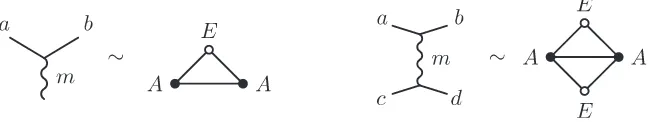
attached to a category like Ak(SU(N)), they do not describe the collection of inter-relations existing between a monoidal categoryAk, a chosen module E, and the endomorphisms O(E) of the later. However, an extension of the recoupling models describing the case ofSU(2) “coupled to matter” of type ADE (module-categories) was sketched in a section of [30]. The main idea was to introduce different marks (labels calledAA,AE orEE) for boundary points representing simple objects of the three different types, and three kind of lines (we choose wiggle, continuous, and dashed) for their morphisms. Another idea was to choose an alternative way for drawing diagrams, by using elementary star-triangle duality. Let us consider a simple example: Take m
a simple object in A, and a a simple object in E, since the former acts on the later (we have a monoidal functor from A to the endofunctors of E) we may consider vertices of type a, m, b
where b is a simple object in E, or more generally we may consider “diffusions graphs” (see Fig. 1). Then, by applying a star-triangle duality transformation, we obtain in the first case a triangle with vertices markedE,A,Aand edges of typeAA,AE,AE. In the second case, we obtain a double triangle (a rhombus) with four edges of type AE, and a diagonal of type AA. Since the endomorphism category O of E also acts on E, we have also vertices of type a, x, b, where x is a simple object of O, and dually, triangles with edges of type EE or AE, or double triangles with four edges of typeAE, and a diagonal of typeEE. One can also introduce vertices of typem,n,p(for triangles AAA) sinceAis monoidal, and trianglesEEE sinceOis monoidal as well. Altogether, there are four kinds of triangles and five types of tetrahedra (pairing of double-triangles) describing generalized 6jsymbols. This framework seems to be general enough to handle all kinds of situations where a monoidal category A is “coupled” to a module E. Of course, for any specific example, we also have specific relations between the graphical elements of the model. The case of SU(2) and its modules was presented in [30], but we are not aware of any printed reference presenting graphical models to study SU(3) coupled to its modules. Fortunately, for the purposes of the present paper, the amount of material that we need from such a model is rather small. Although we are mainly interested in SU(3), we shall actually start with a description of theSU(2) case since it allows us to present most concepts in a simpler framework.
Figure 1. Vertex and diffusion graphs forSU(2) coupled toADE matter.
3.2 Equations for the SU(2) model
3.2.1 The fundamental version
For (SU(2), k) alone, i.e. without considering any action of the categoryAk on a module, and calling σp the simple objects, we have one fundamental object σ=σ1 corresponding classically to the two-dimensional spin 1/2 representation. There is a single non trivial intertwiner (the determinant map) which sendsσ⊗σto the trivial representation. This is reflected in by the fact that σ0 appears on the r.h.s. of the equationσ1⊗σ1 =σ0⊕σ2, where dim(σp) = [p+ 1] where [n] = qqn−q−n
−q−1 withq = exp(iπ/(2+k)). The corresponding projector (antisymmetric) is the Jones
projector σ⊗σ 7→C⊂σ⊗σ. The Frobenius isomorphisms lead to the well known existence of an isomorphism5 betweenσ and its conjugateσ. For this reason, the graphical model uses only
one type of wire, which is unoriented. The fundamental intertwiner C is graphically described by the “cup diagram”: read from top to bottom, it indeed tells us thatσ⊗σcontains the trivial representation (remember that the trivial representation is not drawn). Its adjointC†(the same diagram read bottom-up) is the “cap diagram”, so that the composition of the two gives either an operatorU =C†C fromσ⊗σ to itself (the Jones projector, up to scale, displayed as a
“cup-cap”), or a number β = CC† displayed as a “cap-cup”, i.e. a circle (closed loop). Obviously
U2 = βU. It is traditional to introduce the Jones projector e =β−1U, so that e2 = eand to set U1 =U,U2 = 1l⊗U, Un= 1l⊗ · · · ⊗1l⊗U and en=β−1Un. A standard calculation shows that β is equal to the q-number [2]. The graphical elements of the SU(2) primitive model are therefore rather simple since we have only one relation (see Fig. 2, where the symbol D refers to any diagram) involving a single parameter, the value of the circle.
Figure 2. The circle forSU(2).
3.2.2 The clasp version (bound states version)
The clasp version of theAk(SU(2)) model is slightly more involved: the representationσn=σ⊗n
is not a simple object and according to the general philosophy of graphical models, in their primitive version, being a tensor product of n simple objects, it is described byn points along a boundary line. Its endomorphism algebra (operators commuting with the action of SU(2) or SU(2)q on σn) is the Temperley–Lieb algebra. It is generated by linear combination of diagrams representing crossingless matching of the 2npoints (n points “in” andn points “out” in the wire model, or 2n points along a circle, in the spider model), and generated, as a unital algebra, by cup-cap elementsUi (pairs of U-turns in position (i, i+ 1)). The standard recurrence relation for SU(2), namelyσ⊗σn=σn−1⊕σn+1 (Tchebychev) shows that if n < kthere exists a non-trivial intertwiner from σ⊗σn to σn+1 where σn denotes the irreducible representation of quantum dimension [n+ 1]. The corresponding projector (the Wenzl projector Pn, which is symmetric) is therefore obtained as the equivariant projection of σn to its highest weight irreducible summand σn which is described by a clasp of size n or by a vertical line carrying6 a label n. Its expression is given by the Wenzl recurrence formula: P1 = 1l, P2 = 1l−U1/β,
Pn=Pn−1−[n[n]−1]Pn−1Un−1Pn−1. On the r.h.s. of this equation,Pn−1is understood asPn−1⊗1l. The trace ofPn, described by a loop carrying the label n, isµn= Tr(Pn) = [n+ 1].
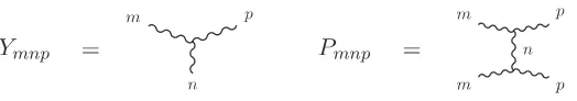
The non-trivial intertwinersYmnp :σm⊗σp 7→σn are described by Y-shaped star diagrams (see Fig.3) with composite wires carrying representation indices (SU(2) weights), or dually, by triangles, where edges are clasps. It is easy to show that the dimension of the triangle spaces is equal to 0 or 1 for allnsince all matrix coefficients (Nn)mpof fusion matrices obtained from the relationNn=Nn−1N1−Nn−2, whereN1is the adjacency matrix of the fusion graphAk+1 =Ak are either equal to 0 or 1. When the value is not 0, the triangle (m, n, p) is called admissible. It can also be associated with an essential path of length n, from the vertexσm to the vertex σp, on the fusion graph (see the discussion in Section3.2.4).
The corresponding endomorphismsPmnp:σm⊗σp 7→σn⊂σm⊗σpare displayed as diffusion graphs of a special kind (see Fig.3), or dually, as particular double triangles. The trace ofPmnp, called theta symbol θ(m, n, p) because of its shape, is represented in Fig. 4. There are general formulae for the values of these symbols, which, for the pureSU(2) case, are symmetric inm,n,p,
6Warning: some authors prefer to denoteσn, notσ
Figure 3. TheY andP intertwiners forSU(2).
see for example [22]; they are obtained by decomposing Ymnp into elementary tangles or along a web basis.
Figure 4. The theta symbol forSU(2).
Composing a Y intertwiner and its adjoint in the opposite order gives a “propagator with a loop” which has to be proportional to the identity morphism ofσnsince the later is irreducible, so that, by evaluating the trace on both sides, one finds the identity displayed7 on Fig. 5. The endomorphisms µn
θ(m,n,p)Pmnp are projectors, as it is clear by composing the P’s vertically:
Figure 5. Normalizing coefficient for aSU(2) loop.
PmnpPmnp =θ(m, n, p)µ−n1Pmnp. Notice the particular caseθ(k−1,1, k) =µk = [k+ 1] so that we recover the Wenzl projectors Pk =Pk−1,k,1, for instance P2 =Y121† Y121 =P121. As a special case, one recovers U =U1=Y101† Y101=P101.
Since the triangle spaces are of dimension 1, the morphism defined by the left-hand side of Fig. 6 should be proportional to the Y-shaped intertwiner Yqpr. This coefficient, that appears† on the r.h.s. of Fig. 6, is written as the product of quantum dimensions and a new scalar quantity called the tetrahedral symbol T ET symbol (the first term). In the “pure” SU(2) theory, quantum or not, the general expression of T ET, which enjoys tetrahedral symmetry as a function of its six arguments, is known [22]. The first three arguments of T ET build an admissible triangle and the last three arguments determine skew lines (in 3-space) with respect to the first three. In the SU(2) theory, this symbol vanishes if m,n, p all refer to the fundamental representation σ because the cube σ3 does not contain the trivial representation. This is precisely what is different in the SU(3) theory.
The (quantum) Racah and Wigner 6j symbols differ from the symbol T ET by normalizing factors. One should be warned that besides T ET, there are at least three types of quantities called “6j” symbols in the literature, even in the pure SU(2) case. The Racah symbols directly enter the structure of the weak bialgebra B associated with the data [30]: For each simple object n one introduces a vector space Hn spanned by a basis whose elements are labelled by admissible triangles8 (with fixed edge n) representing the intertwiners Y
mnp; one defines B=LnBn =LnEnd(Hn). The endomorphism product is depicted by vertical concatenation of vertical diffusion graphs9: Hn(pqrs)Hn′(rtu′s′) = θ(rns)µ
n δnn′δrr′δss′Hn( pq
tu), where the pre-factor is
7To save space, we display it horizontally. 8Or essential paths of lengthnfrommtop.
Figure 6. TheT ET(p n q
s x r) symbol appears as the first term on the right-hand side.
read from Fig. 5. These vertical diffusion graphs represent elementary endomorphisms, up to scale (a pre-factor pθ(p, n, q)θ(r, n, s)/µn). Written in terms of matrices, B is a finite sum of simple blocks labeled by the simple objects n.
Figure 7. Vertical and horizontal diffusion graphs for the pureSU(2) case.
One then introduces horizontal diffusion graphsVx(pqrs), (equivalently, double triangles sharing a horizontal edge), by the equation displayed on the second line of Fig. 7. These new diffusion graphs build a new basis for the same algebra and define a new grading B = LxBx. Using this new basis one introduces a multiplication on the dualBbby concatenation of the horizontal diffusion graphs that can also be used to represent the corresponding dual basis: Vx(pqrs)Vx′(q
′t
s′u) =
θ(qxs)
µx δxx′δqq′δss′Vx( pt
ru). Equivalently this defines a coproduct in B that can be shown to be compatible with the first product. The obtained structure is actually a finite dimensional weak Hopf algebra, a quantum groupoid. The (Racah) symbols{ } used to define the pairing do not enjoy tetrahedral symmetry, but only quadrilateral symmetry. If we set x = 0 in the duality relation (second line of Fig. 7), the tetrahedron degenerates to a triangle and T ET(p n qq0 p) =
θ(p, n, q) that cancels one of the denominators that enters the definition of the Racah symbol, so that one obtains the closure relation Fig.8that will be used later. The proportionality coefficient entering this relation can be simply checked by writing p⊗q =Pn, taking the trace on both sides, the fact that the quantum dimension is a homomorphism, and using the definition of θ.
Figure 8. Closure relation in the pureSU(2) case.
One often defines (Wigner) 6j symbols by the equation
The normalizing factor in the denominator involves the product of theta functions for all trian-gles of the given tetrahedra, so that the 6j symbols [ ] also enjoy tetrahedral symmetry. The terminology is unfortunately not standard: The classical limit of the [ ] symbols are called 6jby most physicists (and Racah 6j by Mathematica) but the{ } are called 6j by [22] and [30]; one can even find, for instance in [3] and in several references studying the geometry of 3-manifolds, a definition of “unnormalized 6j symbols” that differ from T ET, and [ ] by other normalizing factors. The reader may look at [5] for relations between these quantities10 and their use in studying the quantum groupoid structure.
3.2.3 Coupling of SU(2) to ADE matter
If we now coupleSU(2) toADE matter11, the story becomes more complicated (see our general discussion), since we have in general four types of triangles (see Fig.9) and five types of genera-lizedT ET, Racah, or Wigner 6j symbols coupled by pentagonal identities nicknamed “the Big Pentagon” equation (this was commented in [28], see [1]).
Figure 9. The four types of triangles forSU(2) coupled toADE matter.
Since E is a module-category over Ak(SU(2)) we obtain endofunctors of E labelled by the simple objects σn of A, sending objects of E to objects of E. Again, one represents diagram-matically such morphisms fromato bby Y-shaped diagrams calledYanb (see the first diagram on Fig. 10) where a and b refer to simple objects of E. By composition with the upside-down diagrams, we get the second diagram of Fig. 10 that can be traced, as in the pure SU(2) case, to get numbers θanb, see Fig. 11 that replaces Fig.4.
Figure 10. TheY andP intertwiners forSU(2) coupled toADE matter.
Figure 11. The theta symbol forSU(2) coupled toADE matter.
In particular, when nis trivial, the value of the circle associated with an irreducible object aof type E is the corresponding quantum number12 µa (see Fig.12). Composing the morphisms in other directions gives the equations depicted in Fig.13.
Figure 12. The circle for an irreducible objectaof typeE.
10Warning: In this reference the diffusion graphs are rescaled, and the loop has value 1, not [2]. 11Actually toDEmatter since theSU(2) at levelkis theAcase itself.
12In general we callµ
Figure 13. Normalizing coefficients forSU(2) coupled to ADEmatter.
One has to be cautious here because the dimensionality of triangle spaces like anb can be bigger13 than 1; in other words the space of essential paths from a to b and of length n may have a dimension bigger than 1. One should therefore sometimes introduce an extra label α
for vertices such as anb. Comparing the T ET coefficients introduced in Figs. 6 and 14 one notices that m, n, p still label simple objects of Ak(SU(2)), but a, b, c, replacing p, q, x, refer to simple objects of E. The other difference is that the right hand side of Fig. 14 now incorporates a summation over the extra label α, in those cases where the triangle space a,p,b
has a dimension bigger than 1.
Figure 14. TheT ET(a p b
n c m) symbol on the r.h.s. may depend onα,β, γ.
Like in the pure SU(2) case one can introduce a vector space H = LnHn spanned by a basis whose elements are labelled by admissible triangles (with fixed edges n standing for simple objects of Ak(SU(2)) representing intertwiners Yanb. These elements can be interpreted in terms of essential paths fromatob, of lengthn, on the fusion graph ofE (see the discussion in Section 3.2.4). In this SU(2) situation, it is known that H can also be constructed as the vector space underlying the Gelfand–Ponomarev preprojective algebra [16] associated with the corresponding ADE unoriented quiver. With k 6= ∞, identification stems from the fact that dimensions of the finite dimensional vector spacesHn, calculated according to both definitions, are equal (compare for instance [6] and [25]). In the case ofSU(3) considered in the next section, the grading label of the horizontal space Hn refers to a pair of integers n = (n1, n2), seen as a Young tableau, and can no longer be interpreted as a length. When E 6= Ak the ring O(E) is usually not isomorphic with Ak but the construction of the bialgebraB proceeds like in the pureSU(2) case, by using vertical and horizontal diffusion graphs together with the 6j symbols appearing in Fig. 15. We shall not discuss here the structure of B, the interested reader may look at [30,1,36,5,43], but notice that these 6j symbols have four labels for the simple objects of type E (the module), one label for the type A and one label for the type O (the quantum symmetries), whereas the 6j symbols appearing in Fig. 14 have three indices of type E and three indices of type A. Using star-triangle duality, vertices become edges, AA, AE or EE, and the two kinds of 6j symbols just considered belong to the tetrahedral types described in Figs. 16, where black and white vertices refer toA and E marks. If we set x= 0 in the duality relation (second line of Fig. 15), the tetrahedron degenerates and becomes a triangle, like in
13The matrix coefficients of the annular matrices obtained from the relationF
n=Fn−1F1−Fn−2, whereF1is
Figure 15. Vertical and horizontal diffusion graphs forSU(2) coupled to ADEmatter.
Figure 16. Two types of tetrahedra: AAEE andAAAE.
the pure SU(2) situation, and the Racah symbol {a n bd x c} = µn
θ(a,n,b)θ(c,n,d)T ET (a n bd x c) becomes simply {a n bb 0a}= µn
θ(a,n,b). We shall need later theSU(3) analog of this closure relation, which is displayed on Fig. 17.
Figure 17. Closure relation forSU(2) coupled to matter.
3.2.4 SU(2) braiding, Hecke and Jones–Temperley–Lieb algebras
In theSU(2) theory, one also chooses a square rootA= exp(2κiπ) ofqand introduces a braiding14 defined by Fig.18. It reads X=iA1l−iA−1U =ǫ1l +ǫU whereǫ=iA, so thatǫǫ= 1, and U is
Figure 18. The braid relation forSU(2).
the already defined cup-cap generator. Notice thatǫX =−1/q+U. In physics, the braiding can be interpreted as a Boltzman weight at criticality in the context of RSOS height models of type
SU(2). The algebra of the braid group with s+ 1 strands is defined by generators g1, . . . , gs obeying relations gngn+1gn = gn+1gngn+1 and gngm = gmgn when |m−n| ≥ 2. The Hecke algebra with parameter β = [2] =q+ 1/q = 2 cos(π/κ) is obtained as its quotient by the ideal
generated by the quadratic relation (gn+ 1)(gn−q2) = 0. Introducing the change of generators defined by15g
n=q(q−Un), the above three relations defining the Hecke algebra can be written
UnUm=UmUn when |m−n| ≥2,
Un2 =βUn, UnUn+1Un−Un=Un+1UnUn+1−Un+1.
In the SU(2) theory, the operator U is realized as the cup-cap operator appearing on the r.h.s. of Fig. 18. A simple graphical calculation shows that Un actually obeys the stronger equality UnUn±1Un = Un, that replaces the third relation and also ensures the vanishing of a quantum Young projector defined in the algebra of the braid group with three strands (see for instance [10]). The obtained algebra is the Jones–Temperley–Lieb algebraCβs(SU(2)).
In order to better understand what is modified when we trade SU(2) for SU(3), we now remind the reader how to build representations of Cβ(SU(2)) on vector spaces obtained from paths defined on the fusion graph of any module-category E associated with Ak(SU(2)), i.e. on ADE diagrams, or on the fusion graphs of A∞(SU(2)), i.e. SU(2) itself and its subgroups (which are affine ADE diagrams because of the McKay correspondence).
An elementary path is a finite sequence of consecutive edges on a fusion graph of the chosen module E: ξ(1) = ξa1a2, ξ(2) = ξa2a3, etc. Vertices are paths of length 0. The length of the
(possibly backtracking) path (ξ(1)ξ(2)· · ·ξ(p)) is p. We call r(ξcd) = d, and s(ξcd) = c, the range and source of ξcd. For all edges ξ(n+ 1) = ξcd that appear in an elementary path, we set ξ(n+ 1)−1 =. ξdc, and there is no ambiguity since, in theSU(2) theory, all fusion graphs are simply laced. We call Pathpa,b the vector space spanned by all elementary paths of lengthpfrom
a to b. For every integer n > 0, the annihilation operator Cn, acting on elementary paths of lengthp is defined as follows: Ifp≤n,Cn= 0, whereas ifp≥n+ 1 then:
Cn(ξ(1)· · ·ξ(n)ξ(n+ 1)· · ·ξ(p)) =
s
µr(ξ(n))
µs(ξ(n))
δξ(n),ξ(n+1)−1(ξ(1)· · ·ξˆ(n) ˆξ(n+ 1)· · ·ξ(p)).
The symbol “hat”, like in ˆξ, denotes omission. The result is therefore either 0 or a linear combination of elementary paths of length p−2. This definition is extended by linearity to arbitrary elements of Pathpa,b, called “paths”. Intuitively, Cn chops the round trip that possibly appears at position n. A path, not elementary in general, is called essential if it belongs to the intersection of the kernels of the annihilators Cn’s (or of Jones projectors, see below). One introduces a scalar product in the vector space Pathpa,b by declaring that elementary paths are orthonormal. Acting on elementary paths of lengthp, the creating operators Cn† act as follows. Ifn > p+1,Cn†= 0, whereas ifn≤p+1 then, settingc=r(ξ(n−1)),Cn†(ξ(1)· · ·ξ(n−1)· · ·) =
P
|d−c|=1
qµ
d
µc(ξ(1)· · ·ξ(n−1)ξcdξdc· · ·).The previous sum is taken over the neighborsdofcon the fusion graph. Intuitively, this operator inserts all possible small round trip(s) in positionn. The result is therefore either 0 or a linear combination of paths of length p+ 2. In particular, on paths of length zero (i.e. vertices), one obtains: C1†(a) = P|b−a|=1qµb
µaξabξba. The Jones’
projectors en are obtained as endomorphisms of Pathp by en =. β1Cn†Cn. All expected relations between the en, or between the Un = βen, are satisfied, and we obtain in this way a path realization of the Jones–Temperley–Lieb algebra, hence a representation of the Hecke algebra with parameter β. In particular, for every paira,bof neighboring vertices:
U(ξabξba) =
X
{c:|c−a|=1}
√µ bµc
µa
ξacξca
15Another favorite possibility is to take the r.h.s. equal toqU
n−1l which amounts to replace the projectorUn/β
so that for every vertex aof the fusion graph of E, i.e. a simple object of the later, one obtains a representation on the space Path2a,aspanned by elementary paths of length 2 fromatoa(round trips). In theSU(2) theory there are only single edges, they are un-oriented, and vertices have 1, 2 or 3 neighbors. The matrix representative of U is a direct sum of blocks of sizes (1,1), (2,2) or (3,3). OnceU is represented as above, the braiding X can be considered as one of the two fundamental connections (say 1L) attached to the cell system defined by E. Its value on a basic16 cell is:
c d
b a
X = ǫδbc+ǫδadR with R=
rµ
bµc
µaµd
.
The other fundamental connection (1R) is obtained by replacing ǫ by its conjugate ǫin the above expression. Biunitarity of the connection is ensured by the relation ǫ2+ǫ2+β = 0. The quantityRdescribes a kind of generalized parallel transport from top to bottom horizontal edges along the vertical edges. The above basic cell is also a fundamental Racah symbol {a n b
d x c}, for
n= 1 andx= 1L. It gives the pairing of matrix units belonging to the block of the bialgebraB labeled by n= 1, the fundamental representation of Ak(SU(2)), and the block ofBblabelled by
x = 1L, one of the two chiral generators of O = EndAkE. It can be pictured as a tetrahedron pairing a double triangle (anb)(cnd), i.e. a matrix unit of B, and a double triangle (axc)(bxd), i.e. a matrix unit of Bb.
3.2.5 Comment about the SU(2) epsilon tensor
Before embarking onSU(3) let us return to the determinant map (or epsilon tensorǫ) ofSU(2). Call {α1, α2} an orthonormal basis of the representation space associated with the fundamen-talσ. The intertwinerσ⊗σ 7→Cis the epsilon tensorǫ, defined byǫ(αi⊗αj) =ǫij, the signature of the permutation (ij), which is 0 if i=j and ±1 otherwise. Takev, w two vectors in σ, then
ǫ(v⊗w) =ǫijviwj =v1w2−v2w1, which is the determinant det(v, w). One often says that this mapσ⊗σ 7→Cinduces, by duality, an isomorphism fromσtoσ (a particular case of Frobenius isomorphism), but there is a subtlety here: since det is antisymmetric under a circular permu-tation of the columns (a transposition in this case) one does not obtain a single isomorphism fromσ toσ, but two, with zero sum, namely (α1, α2)7→(−α2, α1) and (α1, α2)7→(α2,−α1). In other words, in any wire model ofSU(2) the wires will be unoriented (sinceσ is equivalent to its conjugate), but one should, in principle, use two distinct wires joining boundary points because there are two fundamental intertwiners. Since they have zero sum, it does not harm to make a choice once and for all, so that in practice only one kind of wire is used. The discussion is not modified when we move from SU(2) to SU(2)q. The only place where this subtlety should be remembered is when one tries to define an action of the categoryAk(SU(2)) on a module whose fusion graph would contain tadpoles: the presence of a tadpole – loop – at the vertexa(a simple object) would mean that, besides the identity, we could have another intertwiner from a toa, but they should be proportional sinceais simple, however the sign of this proportionality factor
θ(a,1, a) will change if we select the opposite convention for the isomorphism betweenσ andσ. The only possible conclusion is that the proportionality factor is zero, which means that such a graph cannot be associated with any SU(2) module. This argument was presented in [31]. Another proof eliminating tadpole graphs was given in [35].
3.3 Equations for the SU(3) model
TheSU(3) case shares many features with theSU(2) case. This was one of the reasons to discuss the simpler later case in the previous section, so that we can now concentrate on novel features. Besides the fact that one has to take into account orientation of edges, complex conjugation (non trivial Frobenius isomorphisms), and the fact that have usually a dimension bigger than 1, the general discussion about the structure of the weak bialgebraBand the different types of 6j
symbols stays essentially the same. In particular there are again five types of tetrahedra and therefore five types of cells17, but those that we need to consider here are of type AAAE. As already stated, 6j of that type vanish forSU(2) when the three edgesAA(simple objects ofA) all coincide with the fundamental representation σ, this is precisely what is not true for SU(3).
3.3.1 The elementary version
ForSU(3), we call{α1, α2, α3}the orthonormal basis ofσ. Again, the intertwiner (determinant map) det : σ⊗σ⊗σ 7→ C is defined by the epsilon tensor ǫ(αi⊗αj⊗αk) = ǫijkαk, with ǫijk the signature of the permutation (ijk). Using Frobenius isomorphisms on the identity inter-twiner σ 7→ σ gives an intertwiner σ⊗σ 7→ C represented as a cup diagram. Here σ is not equivalent to σ and the basic wire (representing an intertwiner from σ to itself, or from σ to itself) is oriented: a downward oriented wire, read from top to bottom, denotes the identity morphism fromσ toσ and an upward oriented wire, also read from top to bottom, denotes the identity morphism from σ toσ. The determinant map is symmetric under circular permutation of the columns and the problem discussed for SU(2) at the end of the previous section does not arise. In particular, tadpoles in graphs describing SU(3) modules may exist. Using Frobenius isomorphisms on the determinant map σ3 7→ C leads to an intertwining operator σ⊗σ 7→ σ graphically represented18 by the triple vertex (Fig. 19) with all wires oriented in, and an
inter-twining operatorσ⊗σ7→σ represented by the triple vertex (Fig.19) with all wires oriented out.
Figure 19. The triple vertex forSU(3).
A graphical TQFT model forSU(3) is therefore given by an orientable surface with a finite set of distinguished boundary points, and every such point should have a direction (inner or outer) associated with it. A diagram in the model (primitive version) is a wire diagram made of oriented wires that meet at triple points, or end at boundary points, in a way compatible with the predefined exits (directions associated with boundary points). Notice that triple vertices are not boundary points. Existence of the determinant map, an intertwiner fromσ3 toC, the trivial representation, can be interpreted in terms or the well known representation theory of SU(3), or of quantum SU(3)q. Indeedσ3, which is not irreducible, decomposes as follows into a direct sum (we use highest weights notations for irreducible representations):
((1,0)⊗(1,0))⊗(1,0) = ((0,1)⊕(2,0))⊗(1,0) = ((0,0)⊕(1,1))⊕((1,1)⊕(3,0)).
In terms of classical notations: (3)3 = (3 + 6) 3 = (3 3) + (6 3) = (1 + 8) + (8 + 10), and in terms of quantum dimensions, if the level k is large enough, [3]3 = ([3] + [3][4]/[2])×[3] = ([3]×[3]) + ([3][4]/[2]×[3]) = ([1] + [2][4]) + ([2][4] + [4][5]/[2]).These elementary calculations show that indeed, the trivial representation appears on the r.h.s.
176jsymbols forGat levelkcoupled to a moduleE are often called “Ocneanu cells”. 18{e
We now turn to “relations between relations” (i.e. to relations between intertwiners), there are three of them. The first, reminiscent of theSU(2) theory, says that the circle has value [3]. Indeed, in the SU(3) theory, we have the same cup-cap morphisms as before, but they are now oriented. The cap graph, read from top to bottom, says that there is an intertwiner from the trivial representation to 3⊗3, and the cup graph, read from top to bottom, says that 3⊗3 contains the trivial representation. Composition of the two, from top to bottom, gives a number, i.e. the rule displayed on Fig.20. In the SU(2) theory there are no further relations, but in the
SU(3) theory, there are two.
Figure 20. The circle forSU(3).
First non-trivial relation. Consider the morphism σ7→σ⊗σ 7→σ. Read from top to bottom it is represented by the left hand side of Fig.21. This morphism goes fromσ toσ, howeverσ is irreducible, so this morphism is proportional to the identity morphism. The equality is depicted by Fig. 21. Conventionally the proportionality constant is equal to β =q+ 1/q = [2]. Tracing this equality gives immediately the value of the theta symbol: θ(σ, σ, σ) = [2] [3].
Figure 21. The quadratic relation for SU(3).
Second non-trivial relation. Let us consider the possible morphisms from σ ⊗σ to σ ⊗σ. There are three of them (we suppress the tensor product signs in this discussion):
1. We do nothing, i.e. σ goes to σ and σ goes to σ. It is an identity morphism depicted by the last term on the r.h.s. of Fig.22.
2. We compose the cup and cap morphisms: σ⊗σ → C → σ⊗σ. This is depicted by the first term on the r.h.s. of Fig. 22.
3. The last possibility is to consider the chain depicted by the l.h.s. of Fig. 22:
σ⊗σ→(σ⊗σ)⊗σ=σ⊗(σ⊗σ)→σ⊗σ→(σ⊗σ)⊗σ=σ⊗(σ⊗σ) =σ⊗σ.
Figure 22. The quartic relation forSU(3).
However, as we know,σ⊗σ =σ(1,0)⊗σ(0,1)=σ(0,0)⊕σ(1,1), in terms of highest weights labels (or, in terms of quantum dimensions: [3]×[3] = [1]+[2][4], or, classically, 3×3 = 1+8). So, from
σ⊗σ to itself. This means that the three morphisms found previously cannot be independent: there is a linear relation between them. The third (for instance) can be written in terms of the first two. Actually, as displayed on Fig. 22, the third is justthe sum of the first two, this was shown by [23] where it is also shown that all other relations between morphisms of SU(3) are consequences of Figs. 21and 22. Although belonging to the folklore (we already mentioned the fact that they were explicitly used by [14]) these two relations are often called “quadratic and quartic equations for the Kuperberg SU(3) spider”. The first is called quadratic because it involvestwotriple points and the other is quartic because it involves four triple points. Since these relations hold forSU(3), classical or quantum, they should also hold for any (classical or quantum) module, i.e. they should be true for SU(3) itself, its finite subgroups, for the fusion categories Ak(SU(3)) and their module – categories E.
3.3.2 The clasp version (bound states version)
There is of course a clasp version of the wire models, with new types of wires for every irreducible representation existing at level k. As usual, those “bound states wires” are labelled by highest weights (p, q) or Young tableaux. By looking at the expressions of fusion matrices for SU(3) at levelk, one notices that the dimension of triangle spaces can be bigger than 1, even in the pure
SU(3) case, in contrast with theSU(2) theory. The endomorphism algebra of the objectσm⊗σn, i.e. HomSU(3)(σm⊗σn, σm⊗σn) is theSU(3) version of the Temperley–Lieb algebra. It can be generated by linear combination of diagrams generalizing those discussed in the SU(2) section; one can also define generalizations Pmn of the Wenzl projectors, with image the irreducible representation of SU(3) indexed by the highest weight (m, n), in the endomorphism algebra of σm⊗σn (see [34, 23, 41]), obeying a three terms recurrence relation. One can even define a natural basis in arbitrary intertwiner spaces, see [41], however we shall not need these explicit constructions in full generality. The definition of theta symbols and 6jsymbols then follows the general rules described in theSU(2) section, but this has to be done with much more care because edges are oriented, and also because the dimensiondnof triangle spacesHn, wheren={n1, n2}, is usually bigger than 1, so that the notations, for example, have to incorporates new labels. The recurrence relations for SU(3) fusion matrices Nn = (Nn,p) = (q N(n1,n2),(p1,p2)
(q1,q2)), using
the seed N(1,0), the adjacency matrix of the fusion graph, are:
N(λ,µ)=N(1,0)N(λ−1,µ)−N(λ−1,µ−1)−N(λ−2,µ+1) if µ6= 0, N(λ,0) =N(1,0)N(λ−1,0)−N(λ−2,1), N(0,λ)= (N(λ,0))tr.
As usual, dn=Pp,qNn,p.q
3.4 Coupling to SU(3) matter: Ocneanu coherence equations
for SU(3) triangular cells (self-connections)
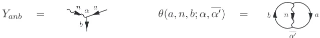
Before deriving these equations we need to consider an extension of theSU(3) recoupling system whereAk(SU(3)) is allowed to act on a moduleE. In a wire model, the solid wire labelledarefers to a simple object of E and the corresponding circle, labelled a denotes its Perron–Frobenius dimension µa. A morphism from a to b, induced from the action of the simple object19 n of Ak(SU(3)) is represented, in the extended wire model, as a vertex anb, see Fig. 23 where the extra index α keeps track of multiplicities. The corresponding theta symbol isθ(a, n, b;α, α′).
The module action ofAk(SU(3)) onEis defined by a fusion graph that will be calledGin the last section: it is the Cayley graph describing the action ofσ =σ(1,0) (the basic representation) on the simple objects, called a, b, . . ., of E. More generally, the action n×a = PbFb
nab of
Figure 23. TheY intertwiner for SU(3) coupled to SU(3) matter and its theta symbol.
the simple objects n of Ak is described by the so-called annular matrices Fn obeying the same recurrence relation as the fusion matricesNn, only the seedG=F(1,0), is different.
For any fusion graphG describing a quantum moduleE of type SU(3), we shall obtain two coherence equations for the system of triangular cells on the graph G. In physicists’ parlance, they are obtained from the two previously discussed Kuperberg equations by couplingSU(3) to E-type matter, and taking a trace.
3.4.1 Normalization and closure relations
When n refers to the fundamental (and basic) representation σ = (1,0) we usually do not put any explicit label on the corresponding oriented line of the wire model diagram, and the morphism a⊗σ → b is described by an oriented edge from a to b on the fusion graph of E. This intertwiner, at the moment, is only defined up to scale, so we need to fix its normalization. This is done by giving a value to the corresponding theta symbol: It is convenient to set:
θ(a, b;α, α′)≡θ(a, σ, b;α, α′) =δ
αα′√µa√µb, depicted by Fig. 24.
Figure 24. Normalization of the fundamental intertwiner.
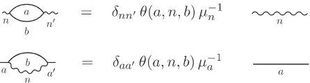
At some point we shall need the following closure relations: Figs.25 and 26. They can be seen as generalizations of those already obtained for SU(2) (see Figs. 8 and 17). Notice that Fig. 26implies µa=Pn(µn/θ(a, n, a;α, α′))µaµaδαα′ so that 1/µa=Pnµn/θ(a, n, a;α, α).
Figure 25. Closure relation 1.
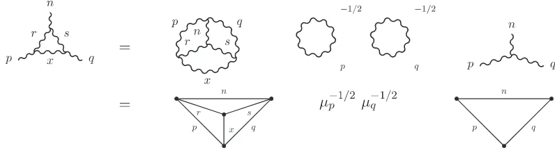
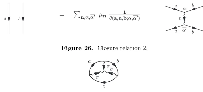
We shall not discuss the extended recoupling theory for SU(3) in full generality, but, as already stressed, we have to associate a number to any elementary oriented triangle of the graph E. This number is a special kind of 6j symbol where three basic representations σ
meet at a triple point on the wire model. It is diagrammatically denoted by the particular tetrahedral symbol T ET(a σ bσ c σ) displayed on Fig. 27. One should compare it with the SU(2) symbolT ET(a p bn c m), on the r.h.s. of Fig.14, which is automatically 0 when allm,n,pcoincide withσ. From now on we shall only consider tetrahedral symbols of that type, called triangular cells since their values Tabcαβγ depend only on trianglesµα,β,γa,b,c on the fusion graph of E, where α,
Figure 26. Closure relation 2.
Figure 27. The elementaryT ET symbol forSU(3) coupled toE-type matter.
3.4.2 The quadratic equation (Type I)
Figure 28. The traced quadratic relation forSU(3) coupled to E-type matter.
We plug the first Kuperberg equation in a loop of type E: see Fig. 28. The right hand side (a theta symbol) is already known. The left hand side, evaluated using first the closure equations Fig.25twice20, with Fig.29appearing at the end of this intermediate step, and then
Figure 29. An intermediate step.
using the closure relation Fig.26once, becomes a sum of products of more elementary diagrams, as described on Fig. 30. Explicitly, the evaluation of the l.h.s. reads21:
l.h.s.=X c
X
d
X
n
µc
θ(a, σ, c)
µd
θ(d, σ, b)
µn
θ(c, n, d)δcdT αβγ abc T
α′βγ
abd
=X
c
X
n
µc
θ(a, σ, c)
µc
θ(c, σ, b)
µn
θ(c, n, c)T αβγ abc T
α′βγ
abc
=X
c
µc
θ(a, σ, c)
µc
θ(c, σ, b)µc
−1 TabcαβγT
α′βγ
abc
=X
c
θ(a, σ, c)−1µcθ(c, σ, b)−1TabcαβγT α′βγ
abc .
20Heren=σ, the fundamental representation.
Figure 30. The left hand side of the traced quadratic equation.
On the first line, we have replaced one tetrahedral symbol by its conjugate, using the equality displayed on Fig. 31.
Figure 31. Relation betweenT andT.
The sum over µn/θ(c, n, c) on the second line was replaced by µc−1 from the last equality obtained in Section 3.4.1. We did not write explicit labels on arcs and vertices of Fig. 30, but a summation should be carried out, not only on the arcs ebut over all “dummy vertex labels”, i.e. those not already labelling the vertices of Fig.28. It is clear that the sequence of operations is easier to follow when it is displayed graphically; this is what we shall do later when we come to discuss the quartic equation.
Usingθ(a, σ, c) =√a√c in the above, the left and right hand sides give respectively
l.h.s.=X c
1 õ
c 1 õ
b TabcαβγT
α′βγ
abc , r.h.s.= [2]õaõb.
So that one obtains finally the following equality:
X
c,β,γ TabcαβγT
α′βγ
abc = [2]δαα′µaµb.
3.4.3 The quartic equation (Type II)
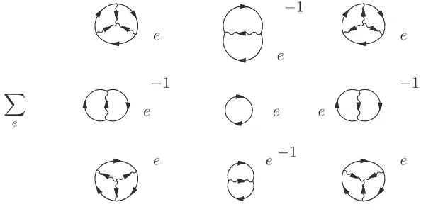
Figure 32. The traced quartic relation for SU(3) coupled toE-type matter.
or loops. When written in terms of TQFT wires (graphs), the left hand side of the quartic equation therefore decomposes as a sum of products involving four tetrahedral symbols, four inverse “propagators” θ(which are proportional to Kronecker deltas) and one loop (a quantum dimension). This is displayed on Fig. 33.
Figure 33. The left hand side of the traced quartic equation.
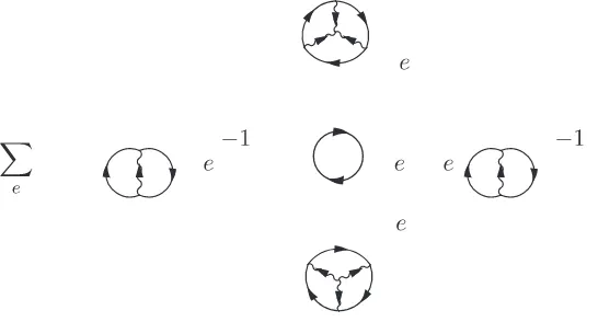
On the right hand side, the calculation is simpler. One only has to use the closure equations of Fig.26on each of the two terms, together with the fact that only the intermediate staten= 0 contributes. We obtain in this way a sum of two terms (Fig.34) where each term is a product of two theta symbols. As usual, each such symbol gives a delta function and a product of square roots of quantum dimensions. After simplification, and using the equation of Fig.31that relates a tetrahedral symbol with its conjugate, one gets22:
X 1
µeT β1β2α2
aeb T β1β4α1
aed Tcedβ3β4α4T β3β2α3
ceb =δα1α2δα3α4µaµbµc+δα1α4δα2α3µaµcµd.
The diagrammatic interpretation of this equation, in terms of the triangles of a fusion graph, is actually simpler than what it looks. We shall return to it later.
Figure 34. The right hand side of the traced quartic equation.
3.4.4 Gauge freedom
Coherence equations of Types I and II usually do not determine completely the cell values of the triangles of a fusion graph. More precisely, given a solution, i.e. a coherent assignment of complex numbers to all triangles of the graph, one can construct other solutions by using arbitrary unitary matrices of size sab ×sab, where sab denote the multiplicity of edges going from vertex a to vertex b. In particular, for graphs with single edges, a gauge choice associates phase factors to edges. The effect of a gauge transformation is to multiply the values of triangular cells sharing a given edge (simple or multiple) by the chosen unitary factors. This will be illustrated later.
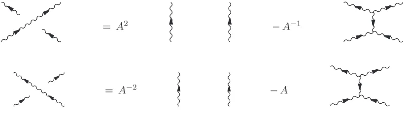
3.4.5 SU(3) braiding, Hecke and generalized JTL algebras
In the SU(3) theory, one also chooses a cubic rootA = exp(3κiπ) of q and introduces a braiding defined by Fig. 35. It reads X = A21l−A−1U where U now denotes the double-triple vertex
Figure 35. The braid relation forSU(3).
of SU(3) that replaces the SU(2) cup-cap generator. The SU(3) wire model, in its primitive version, using the graphical elements presented in Section3.3.1, is defined by the three relations displayed in Figs.21,22,35. The operatorsUn= 1l⊗· · ·⊗1l⊗U generate an algebraCβ(SU(3)); they still obey the defining relations of the Hecke algebra with parameter β = q +q−1 (see Section3.2.4), in particular U2=βU, but with an extra relation that replaces the usualSU(2) Jones–Temperley–Lieb relation. It reads: (U3U2U1 −(U1+U3))(U2U3U2 −U2) = 0 and can be obtained by imposing the vanishing of a quantum Young projector defined in the algebra of the braid group with four strands (see for instance [9] or [10]). Notice that Cβ(SU(2)) ⊂
Cβ(SU(3)). The operator F = U1U2U1−U1 pictured on Fig. 36 is also of interest. Simple graphical calculations show that Fn2 = [2][3]Fn, FnFn±1Fn = [2]2Fn and FiFj = FjFi when |i−j| > 2, but, as noticed in [13], the operators Fn do not generate an algebra isomorphic withCβ(SU(2)) because the last commutation relation fails for|i−j|= 2. As withSU(2), one can represent the SU(3) intertwiners on vector spaces of paths defined on the fusion graph of any module-category E associated withAk(SU(3)), or on the fusion graphs ofA∞(SU(3)), i.e.
SU(3) itself and its subgroups. The fusion graphs are now oriented: one graph is associated with the action ofσ, and another one, with opposite orientation, describes the action ofσ. From now on, for definiteness, we choose the first. These graphs still obey the rigidity constraint that, in the SU(2) case, implies the condition of being simply laced, but now, there may be more than one (oriented) edge ξab between verticesa and b, and for this reason it is usually denoted ξabα. An elementary path could be defined as a succession of matching edges ξα
Figure 36. The operatorF. Figure 37. From triangular cells to Hecke.
on paths containing both types of edges, as it is clear from its definition, reads:
Cn(ξ(1)· · ·ξ(n−1)ξabαξ β
bcξ(n+ 2)· · ·ξ(p))
=X
γ
Tabcαβγ √µ
aµc
(ξ(1)· · ·ξ(n−1)ξacγ ξ(n+ 2)· · ·ξ(p)).
Formally, the prefactor, that waspµb/µafor a singleSU(2) elementary round tripξabξbais now replaced, for an SU(3) elementary triangle ξabαξbcβξca, by the prefactorγ Tabcαβγ/√µaµc. Compo-sing C with its adjoint gives the operator U: for every integern >0, Un, as an endomorphism of Pathp, acts as follows on elementary paths with arbitrary length, origin and extremity:
Un(ξ(1)· · ·ξ(n−1)ξabαξbcβξ(n+ 2)· · ·ξ(p))
=X
α′β′
Uαβα′β′(ξ(1)· · ·ξ(n−1)ξα
′
ab′ξβ ′
b′cξ(n+ 2)· · ·ξ(p)),
where
Uαβα′β′ =
X
γ 1
µaµcT αβγ abc T
α′β′γ
ab′c .
The last summation runs over all edges γ such that (ξabαξbcβξca) and (γ ξabα′′ξβ ′
b′cξca) make a rhombusγ
with diagonal γ, i.e. a pair of elementary triangles sharing the edge ξcaγ from c toa.
A matching pair of edges (αβ) determines three verticesa,b,cof a triangle, so that when the triangular cellsTabcαβγ are known, the above equation associates to every pair (a, c) of neighboring vertices of the fusion graph an explicit square matrix whose lines and columns are labelled by triangles sharing the given two vertices. Its matrix elements associate C-numbers to the various, possibly degenerated, rhombi with given diagonal (only its endpoints are given). This representation of the Hecke algebra can sometimes be obtained by other means: there are general formula for representations associated with Ak(SU(N)) itself, given in [44], and all Hecke representations associated with modules over Ak(SU(3)) were obtained by “computer aided flair” in [9]. The point to be stressed is that the obtained representation is now deduced
from the values of triangular cells. This was discussed in [12]. For illustration we shall only give one example of this construction (see the end of Section4.3.2).
4
Triangular cells on fusion graphs
4.1 Self-connection on graphs
An SU(3) module E at level k is specified by its fusion graph, also called E. The adjacency matrix, called G, encodes the action of the fundamental generator σ = σ(1,0) of Ak(SU(3)) on the simple objects a, b, c, . . . of E, represented as vertices. There exist a Perron–Frobenius positive measure on the set of vertices, it gives their quantum dimension denoted23 [a] =µa for the vertex a.
We consider the following oriented triangles of the fusion graph:
a b set of oriented triangles of Gto the complex numbers, that we denote as follows:
T
The complex numbers Tabcαβγ are the triangular cells of G or simply “cells” in the sequel, since they will all be of that type. As discussed previously, in order to guarantee the existence of a module-category E described by the fusion graphG, the set of triangular cells associated with this graph has to obey the following coherence equations.
Type I equations. For each frame24 a α b
α′ of the graph G, ie a double edge α, α ′
from atob, we have a quadratic equation (or “small pocket equation”):
T
Type II equations. For each frame25
a1 a4
23Warning: in the previous sections, this was the notation forq-numbers but there should be no confusion. 24It may be degenerated, it is then a single edge.
Gauge equivalence. Let T be a cell system for the graph G. For any pair of vertices a, b
ofG, let the integersab denote the edge multiplicity fromatoband letUab be a unitary matrix of size sab×sab. We define the complex numbers:
These complex numbers satisfy Type I and Type II equations, thereforeT′ is also a cell system for the graphG. The two cell systems are called gauge equivalent. An equivalence class of cell systems is called a self-connection onG. A quantity is an invariant of the cell-system if its value does not depend on the gauge choices.
4.2 Solving the cell system
The number of edges from a given vertex a to a given vertex b is equal to the matrix-ele-ment (G)ab. The number of cells of G is 13Pa(GGG)aa = 13Tr(G3). These complex numbers have to satisfy Type I and Type II equations. There is one Type I equation for each pair of vertices linked by one (or more) edge(s). So the number of Type I equations is given by the number of non-zero matrix elements of G. For Type II equations, the number of frames is given by Tr(GGTGGT) whereGT is the transpose matrix ofG. But the following frames (related by the two diagonal symmetries):
lead to the same equations, so the number of Type II equations is reduced26.
The number of Type I and Type II equations is much larger than the number of cells that one has to compute. Nevertheless, these equations do not fix completely their values and one can make use of gauge freedom for that. In the examples treated, we try to choose the most convenient solution (either by imposing real values for the cells, if possible, or by making a gauge choice exhibiting the symmetry of the graph). The resolution technique for a cell system depends largely on the chosen example.
4.2.1 Graphs with single edges
Most fusion graphs of SU(3) have only single edges (exceptions are the A∗ and D3s series, the special twisted conjugate Dtc
9 and the exceptional E9). Since there is no multiplicity, we can drop the edge labeling symbols and denote the cells simply byTabc. The cell values, on a given triangle, for two gauge equivalent cell systems T and T′ will only differ by phase factors since the unitary matrices in (2) are one-dimensional in this case.
(i) Type I equations. Sinceα =α′, these equations reduce to:
X
c
|Tabc|2 = 2q[a][b],
and only give quadratic constraints on the modulus of the cells.
26Even after considering diagonal symmetries, two different frames can lead to the same equation. In some