Goodness of fit procedures for the
multivariate linear model based on
spherical harmonics
Pruebas de bondad de ajuste para el modelo lineal
multivariado basadas en arm´
onicas esf´
ericas
A. J. Quiroz (
[email protected]
)
Universidad Sim´on Bol´ıvar
Valle de Sartenejas, Baruta, Edo. Miranda, 1080A.
J. M. Tapia (
[email protected]
)
UNELLEZ, Barinas
Av. 23 de enero, Barinas, Edo. Barinas
Abstract
The theory of the goodness of fit procedures for multivariate nor-mality based on spherical harmonics, introduced in [6], is extended to cover the context of the multivariate linear model (MLM). The limiting distribution of the statistics considered does depend on the distribution of the covariates in the MLM, and our results provide a complete de-scription of the manner in which the covariate distribution affects the goodness of fit statistics. We provide two methods for approximation of the limiting distributions when, as is usually the case, the covariate dis-tribution is unknown, and evaluate their performance in simulations.
Key words and phrases: Conditional models, empirical processes, Goodness of fit testing.
Resumen
La teor´ıa de los m´etodos de bondad de ajuste para la familia normal multivariada, basados en arm´onicas esf´ericas, presentada en [6], se ex-tiende, en el presente trabajo, al contexto del modelo lineal multivaria-do (MLM). Nuestros resultamultivaria-dos proporcionan una descripci´on completa
de la distribuci´on l´ımite de los estad´ısticos considerados, incluyendo la manera en que la distribuci´on de la covariable afecta dicha distribu-ci´on l´ımite. Describimos dos m´etodos para la obtenci´on de cuantiles aproximados para los estad´ısticos considerados (cuando se desconoce la distribuci´on de la covariable) y evaluamos el desempe˜no de estos m´eto-dos mediante simulaciones.
Palabras y frases clave:Modelos condicionales, procesos emp´ıricos, pruebas de bondad de ajuste.
1
Introduction
In recent years, a number of meaningful and effective methods have been developed for testing the null hypothesis of multivariate normality. Among these, we would like to mention the statistics obtained from kernel density estimators of Bowman and Foster [3], the statistics that use the empirical characteristic function of Henze and Wagner [4] and the statistics based on spherical harmonics and radial functions studied by Manzotti and Quiroz [6]. These statistics join the classic procedures of Mardia [7] among the best tools for deciding on the question of multivariate normality.
It seems natural to try to adapt the best of the test statistics for multivari-ate normality to the problem of testing for the adequacy of the Multivarimultivari-ate Linear Model (MLM, also referred to as the General Linear Model [1]) in the context of models with covariates, by applying the tests for multivari-ate normality to the residuals of the fitted conditional model. In doing so, some caution must be exerted, since the covariate distribution could affect the distribution of the test statistics being used.
When assessing goodness of fit of the MLM, it is common practice to informally examine the residuals for lack of uniformity, that is often associated with lack of independence between the radial and directional components of the residuals. In this respect the statistics proposed in [6] and, in particular, their Z2
2,n, is well suited to detect this kind of departures from multivariate
normality. Thus, the main goal of the present article is to carry out the adaptation of this statistic to the context of goodness of fit for the MLM. For this purpose we will describe a generalization of Theorem 2 in [8] and provide procedures for estimation of quantiles under minimal assumptions when the covariate distribution is unknown.
In order to present the statistic that we will consider, we will first intro-duce some notation. Let (X1, Y1), . . . ,(Xn, Yn) be an i.i.d. sample from the
probability law P onIRp×IRq. TheX′
random vectors inIRp (resp.IRq). In the MLM, the conditional assumption (the null hypothesis that we want to test) is that, given Xi,
Yi=B Xi+Zi (1)
where B is a q×pparameter matrix and Zi ∈IRq has distribution N(0,Σ),
for an unknown positive definite covariance matrix Σ. Let us denote byµthe marginal distribution (onIRp) of X1 and byP =P0 the joint distribution of the pair (X1, Y1) under the null distribution. LetX(resp. Y) denote theX (resp. Y) sample written in matrix form: Xis ann×pmatrix in which each
Xiappears as a row. Then, as is well known (see, for example, [1]), the MLE
forθ0= (B,Σ), namely, ˆθ= ( ˆB, S), is given by
θ the joint distribution of a vector
(X, Y) for whichX has distributionµ and the conditional distribution of Y
givenX is N( ˆB X, S). The standardized residuals are the vectorsS−1/2(Y
i−
ˆ
BXi).
The statistic we want to consider is obtained by application, to the stan-dardized residuals, of radial functions and spherical harmonics described next. Let Ωq ={y ∈IRq :kyk = 1} be theq-dimensional unit sphere. A spherical
harmonic of degreejis the restriction to Ωq of a homogeneous polynomialp(y)
onIRq, of degreej, such that ∆(p)≡0 onIRq, where ∆ denotes the Laplace
operatorPq
i=1∂ 2
/∂x2
i. In dimension 2, the spherical harmonics coincide with
the trigonometric functions on the unit circle. In higher dimensions, as in di-mension 2, their linear combinations are dense, with respect to the sup norm, in the space of continuous functions on Ωq [9]. In [6] closed form formulae
have been worked out for the spherical harmonics of degree up to 4, in an or-thonormal basis with respect to the uniform probability measure on the unit sphere. We will denote Ej the set of spherical harmonics of degree j in this
orthonormal basis. The number of linearly independent spherical harmonics of degree j, in dimension q, is given by LI(q, j) = ¡q+j−1
y6= 0 in and a positive integerj, define the functions
rj(y) =kykj and u(y) =y/kyk. (3)
standardization transformation by
Tn(x, y) =S−1/2(y−Bxˆ ). (4)
It is convenient to define, as well, the asymptotic transformation
T∞(x, y) = Σ−1/2(y−Bx). (5)
We will apply to the sample pairs (Xi, Yi), functions which are products of
spherical harmonics and powers of the radial component: (rj◦Tn)(p◦u◦Tn),
where pis a harmonic spheric inEl, 0≤l≤2, andrj anduare as defined in
(3). Based on power considerations, we will use, specifically, the functions (r3◦Tn)(p◦u◦Tn), r1◦Tn andr3◦Tn, (6)
where p ∈ E1 ∪ E2, and these spherical harmonics are listed in the same order as in Table 1 of [6]. This gives a total of k=¡q+1
2
¢
+q+ 1 functions. The functions just introduced will be denoted hj,n,1 ≤ j ≤ k. Under the
null hypothesis, we have consistency of ˆθ and the functionshj,n converge, in
L2(P), to the limitingh
j,∞, obtained by replacingT∞ forTn in (6). Denote
by hn the vector of functions (h1,n, . . . , hk,n)t and by h∞ the corresponding
vector of thehj,∞. For each functionh∈L2(P), let
P h=
Z Z
h(x, y)dP(x, y), Pθˆh=
Z Z
h(x, y)dPθˆ(x, y)
Pnh=
1
n X
i≤n
h(Xi, Yi), νn(h) =√n(Pnh−P h)
and ˆνn(h) =√n(Pnh−Pθˆh). (7) For the vector hn defined above, let ˆνn(hn) = (ˆνn(h1,n), . . . ,νˆn(hk,n)) and
define, similarly, νn(h∞) = (νn(h1,∞), . . . , νn(hk,∞)). The functions in h∞
are fixed, as opposed to those in hn that depend on the sample through the
estimates ˆB and S. Thus, the covariance matrix, under the null hypothesis, of the vector h∞, can, in principle, be calculated in advance. Call M0 this covariance matrix that, in our case, due to our particular choice of functions, turns out to be computable in closed form and coincides with matrix V of formula (2.18) in [6]. Then, the statistic that we will consider is the quadratic form
Zn2= ˆνnt(hn)M
−1
0 νˆn(hn). (8)
In the following section we present some properties of the statistic Z2
n,
including its asymptotic distribution and, in Section 3, we discuss bootstrap procedures for getting approximate quantiles of Z2
2
Invariance and limit distribution of
Z
n2We will now state, without proofs, some results regarding the calculation and distribution ofZ2
n. These results generalize those obtained in [6] and show how
the covariate distribution affects the distribution of the statistic considered. Proofs, based mostly on methods from empirical processes (as described, for instance, in [11]), will appear elsewhere [10].
By our choice of functions, a simplification occurs in the computation of ˆ
νn(hn). When calculatingPθˆhj,n, we need to average, with respect toµ, the
integral
Z
(r3◦Tn)(p◦u◦Tn)(x, y)dN( ˆBx, S)(y). (9)
Noticing that the estimators ˆB and S appear both in the definition of Tn
and in theN( ˆBx, S) distribution, we get, through a change of variables, that the integral in (9) takes the value R
r3(y)p(y/kyk)dN(0, Iq)(y). This last
expression is straightforward to compute and not random!. Our process ˆνn
can be decomposed as
ˆ
νnhj,n=νnhj,n+√n(P hj,n−Pθˆhj,n). (10)
Always assuming the null hypothesis, writeYi=BXi+ Σ1/2Ui, where the
Ui have the standard Gaussian distribution in IRq. Let ˆBU and SU be the
estimators of the parametersB and Σ for the sample (X1, U1), . . . ,(Xn, Un).
(For this hypothetical sample, B is the zero matrix and Σ = Iq). It is not
difficult to verify that these estimators relate to those for the original sample through ˆB =B+ Σ1/2ˆ
BU andS= Σ1/2SUΣ1/2. It follows that the
standard-ized residuals S−1/2
(Yi−BXˆ i) relate to the corresponding residuals for the
(Xi, Ui) sample via
S−1/2
(Yi−BXˆ i) =ρS−
1/2
U (Ui−BˆUXi) (11)
where ρ= (Σ1/2S
UΣ1/2)−1/2Σ1/2S
1/2
U . Sinceρ is an orthogonal matrix and
the functions applied to the residuals are products of radial functions and spherical harmonics, it follows as in [8], Proposition 8, that the distribution of ourZ2
n does not depend on the underlying parametersB and Σ. Thus, we
have a further simplification in the analysis of Z2
n in the sense that we can
assume, in what follows, that the true parameters areB =0and Σ =Iq.
We will now introduce some definitions needed to describe the limiting distribution of Z2
evaluated at u. Putξ0(x, u) =ξ(x, u)|B=0,Σ=Iq. Let us give an order to the the vector of partial derivatives ofξ(x, u) with respect to the parameters listed above (in the order just given), evaluated at B = 0,Σ =Iq. For eachj ≤k, J and the matrixCcan be worked out in terms of moments of the covariate, as follows: Let τ = (µ(X1,1), . . . , µ(X1,p)) (a row vector of moments) and
where the block MX appears qtimes in the diagonal ofJ, as does the vector
d0τ in the ‘diagonal’ ofC;d0=√q(q+ 2),d1=
√
2(q+ 1)(q+ 3)β/p
Generalizing Theorem 2 in [8], we have that the limiting distribution of ˆ
νn(hn) isk-dimensional Gaussian with mean zero and covariance matrixM0−
CJ−1Ct, and, therefore the distribution ofZ2
n converges to that of k
X
j=1
δjWj2 (17)
where theWj are i.i.d. N(0,1) variables and theδj are the eigenvalues of
I−M0−1/2CJ
−1
CtM0−1/2. (18) From this result and the formulas forJ andCin (15) and (16), we see how the covariate moments enter the distribution of our statistic, although it has been computed on ‘residuals’. Since we do not assume a distributional form for the covariate, the moments that appear inτ andMX must be estimated from the
sample. That the null distribution of Z2
n can indeed be effectively estimated
without knowing the covariate distribution is illustrated in the simulations that we describe next.
3
Bootstrapping quantiles of
Z
n2We will now describe a Monte Carlo experiment, performed to evaluate the convergence ofZ2
nto its limiting distribution and the influence of the covariate
distribution on it. We will also present a parametric bootstrap procedure that approximates very closely the null finite sample distribution ofZ2
n. Our setting
is as follows: we take p= 3 andq= 4. Without loss of generality, we assume
B =0and Σ =Iq. For our first example, we generate the 3-dimensional
co-variate from the one parameter multico-variate Burr-Pareto-Logistic distribution whose density is given in [5], formula (9.10), with parameterλ= 0.5. In our second example the covariate has independent coordinates with the student’s
t4 distribution. The first distribution considered has bounded support and correlated coordinates, while the second distribution has relatively heavier tails and independent coordinates.
To approximate the finite sample null distribution of Z2
n, for different
sample sizes ranging from n = 20 to n = 200, and each of the two covari-ate distributions considered, we genercovari-ated (using the R Statistical Language) 10,000 samples of Xis. Then, theYis were generated according to the MLM
(1). For each sample, ˜νn(hn) andZn2 were computed (with code in the R
lan-guage available from the authors) and finite sample quantiles were extracted. These quantiles are displayed in Tables 1 and 2, in rows labeled Z2
Assuming no knowledge of the covariate distribution, the limit distribu-tion can be approximated as follows: We take one sample (the ‘actual sample’) and from theXis we estimate the moments that go in the definitions ofτand
MX. Then we plug these estimates in (15) and (16), and we can compute
an approximation to the matrix in (18). Call the eigenvalues of this matrix ˆ
δj, j ≤k. Then, we can use Monte Carlo quantiles ofPkj=1δˆjW 2
j (based on
10,000 samples of Wjs) as approximate quantiles for the limit distribution.
This procedure was implemented for the sample sizes and covariate distri-butions considered (using only the first covariate sample) and the quantiles obtained are displayed in Tables 1 and 2 in the rows labelledZ2
∞.
Finally, a different approximation to the finite sample quantiles ofZ2
n can
be obtained through a parametric bootstrap, conditioning on the observedXi
sample. For l = 1 to 10,000 generate the null Yi sample according to (1),
using B =0 and Σ =Iq (recall that this does not affect the distribution of
our statistic). Then, compute the corresponding Z2
n for these 10,000 samples
and extract quantiles. This method will produce quantiles that converge, as n → ∞, to the limiting quantiles ofZ2
n (a justification can be obtained
with arguments similar to those in [2]). This bootstrap approximation was implemented (again, based on just one covariate sample for each sample size) and the quantiles obtained are displayed in Tables 1 and 2 in rows labeled
Z2
n,b.
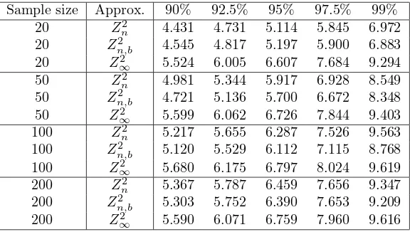
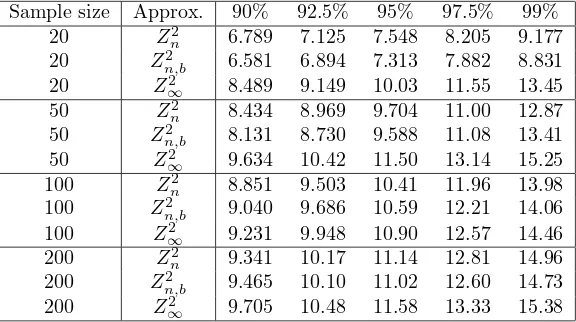
From the results of these simulations we can conclude the following: In the case of the Burr-Pareto-Logistic distribution with bounded support, the limit-ing quantiles (rows Z2
∞) display little variability with sample size, suggesting
that, in this case, a good approximation to the limiting distribution can be attained even with small samples. There is more variability among these rows in Table 2, as could be expected. Still, in both cases, the finite sample quan-tiles ofZ2
n are approaching the approximate limiting quantiles from below, as
n grows. Thus, use of the approximate asymptotic quantiles will produce a conservative procedure, as is usually the case with this type of statistics. In both cases, the agreement between approximate finite sample quantiles, Z2
n,
and limiting quantiles, Z2
∞, becomes fairly acceptable forn ≥ 200. On the
other hand, for both distributions of the covariate, the parametric bootstrap procedure seems to provide a good approximation to the finite sample dis-tribution of Z2
n for all the sample sizes considered. This could be expected,
since the parametric bootstrap is simulating the finite sample statistic and not the asymptotic distribution. On the other hand, the approximate asymptotic quantiles are significantly less expensive from the computational viewpoint. Each number in the Z2
∞ rows takes a couple of seconds of computation on
a desktop PC, while the corresponding numbers in row Z2
require about 15 mins of computation on the same machine. The code in the R statistical language that implements the test statistics and the bootstrap procedures described here is available from the authors.
One important conclusion we can extract from these simulations is that the distribution of Z2
n is significantly affected by the covariate distribution,
as we can judge by the differences between corresponding entries in Tables 1 and 2. This result is a bit surprising, considering that the spherical har-monics and radial functions are applied to the standardized residuals. In this regard, the theory presented in this article is useful in telling us how the co-variate effect appears, and how to obtain valid approximate quantiles forZ2
n
by appropriately using the information contained in the covariate sample.
Table 1: MC quantile approximations for Z2
n, p = 3, q = 4, m = 10
4 ,
X ∼MultivB-P-L(0.5)
Sample size Approx. 90% 92.5% 95% 97.5% 99%
20 Z2
n 4.431 4.731 5.114 5.845 6.972
20 Z2
n,b 4.545 4.817 5.197 5.900 6.883
20 Z2
∞ 5.524 6.005 6.607 7.684 9.294
50 Z2
n 4.981 5.344 5.917 6.928 8.549
50 Z2
n,b 4.721 5.136 5.700 6.672 8.348
50 Z2
∞ 5.599 6.062 6.726 7.844 9.403
100 Z2
n 5.217 5.655 6.287 7.526 9.563
100 Z2
n,b 5.120 5.529 6.112 7.115 8.768
100 Z2
∞ 5.680 6.175 6.797 8.024 9.619
200 Z2
n 5.367 5.787 6.459 7.656 9.347
200 Z2
n,b 5.303 5.752 6.390 7.653 9.209
200 Z2
Table 2: MC quantile approximations for Z2
n, p = 3, q = 4, m = 10
4 , X: independent coordinates t4
Sample size Approx. 90% 92.5% 95% 97.5% 99%
20 Z2
n 6.789 7.125 7.548 8.205 9.177
20 Z2
n,b 6.581 6.894 7.313 7.882 8.831
20 Z2
∞ 8.489 9.149 10.03 11.55 13.45
50 Z2
n 8.434 8.969 9.704 11.00 12.87
50 Z2
n,b 8.131 8.730 9.588 11.08 13.41
50 Z2
∞ 9.634 10.42 11.50 13.14 15.25
100 Z2
n 8.851 9.503 10.41 11.96 13.98
100 Z2
n,b 9.040 9.686 10.59 12.21 14.06
100 Z2
∞ 9.231 9.948 10.90 12.57 14.46
200 Z2
n 9.341 10.17 11.14 12.81 14.96
200 Z2
n,b 9.465 10.10 11.02 12.60 14.73
200 Z2
∞ 9.705 10.48 11.58 13.33 15.38
References
[1] Anderson, T. W. An Introduction to Multivariate Statistical Analysis. Wiley, New York, 2003.
[2] Andrews, D. W. K. A conditional Kolmogorov test. Econometrica 65,
1097-1128, 1997.
[3] Bowman, A. W., Foster, P. J. Adaptive smoothing and density-based tests of multivariate normalityJournal of the American Statistical Asso-ciation88no. 422, 529-537, 1993.
[4] Henze, N., Wagner, T. A new approach to the BHEP tests for multivari-ate normality.Journal of Multivariate Analysis62, 1-23, 1997.
[5] Johnson, M. E.Multivariate Statistical Simulation. John Wiley and Sons, New York, 1987.
[6] Manzotti, A. and Quiroz, A. J. Spherical harmonics in quadratic forms for testing multivariate normality.TEST10, 87-104, 2001.
[8] Quiroz, A. J. and Dudley, R. M. Some new tests for multivariate normal-ity.Prob. Theo. and Rel. Fields87, 521-546, 1991.
[9] Stein, E. M. and Weiss, G.Introduction to Fourier Analysis on Euclidean Spaces. Princeton University Press, Princeton, 1971.
[10] Tapia, J. M.El proceso emp´ırico condicional en bondad de ajuste a mod-elos con covariables. Tesis Doctoral. Universidad Central de Venezuela. To appear, 2006.