THE MINIMUM RANK PROBLEM OVER FINITE FIELDS∗
JASON GROUT†
Abstract. The structure of all graphs having minimum rank at mostkover a finite field withq
elements is characterized for any possiblekandq. A strong connection between this characterization and polarities of projective geometries is explained. Using this connection, a few results in the minimum rank problem are derived by applying some known results from projective geometry.
Key words. Minimum rank, Symmetric matrix, Finite field, Projective geometry, Polarity
graph, Bilinear symmetric form
AMS subject classifications.05C50, 05C75, 15A03, 05B25, 51E20.
1. Introduction. Given a fieldFand a simple undirected graphGonnvertices (i.e., an undirected graph without loops or multiple edges), let S(F, G) be the set of symmetricn×nmatricesAwith entries inF satisfyingaij 6= 0,i6=j, if and only if
ij is an edge in G. There is no restriction on the diagonal entries of the matrices in
S(F, G). Let
mr(F, G) = min{rankA | A∈S(F, G)}.
Let Gk(F) = {G | mr(F, G)≤k}, the set of simple graphs with minimum rank at mostk.
The problem of finding mr(F, G) and describing Gk(F) has recently attracted considerable attention, particularly for the case in whichF =R(see [29, 17, 26, 25,
27, 13, 33, 5, 9, 22, 2, 11, 6, 7, 10, 18, 4]). The minimum rank problem over R is
a sub-problem of a much more general problem, the inverse eigenvalue problem for symmetric matrices: given a family of real numbers, find every symmetric matrix that has the family as its eigenvalues. More particularly, the minimum rank problem is a sub-problem of the inverse eigenvalue problem for graphs, which fixes a zero/nonzero pattern for the symmetric matrices considered in the inverse eigenvalue problem. The minimum rank problem can also be thought of in this way: given a fixed pattern of off-diagonal zeros, what is the smallest rank that a symmetric matrix having that pattern can achieve?
∗Received by the editors January 17, 2008. Accepted for publication July 13, 2010. Handling
Editor: Robert Guralnick.
†Department of Mathematics and Computer Science, Drake University, 2507 University Avenue,
Des Moines, IA 50311, USA ([email protected]).
1
2 3
4 5
Fig. 1.1: A labeled full house graph
Up to the addition of isolated vertices, it is easy to see that G1(F) = {Kn |
n ∈ N} for any field F. In [9] and [10], G2(F) was characterized for any field F
both in terms of forbidden subgraphs and in terms of the structure of the graph complements. The forbidden subgraph characterizations in these papers used ten or fewer graphs for each value ofk. Restricting our focus to finite fields, letFq denote
the finite field with qelements. Ding and Kotlov [18] independently used structures similar to the structures that we use in this paper to obtain some special cases of some structural results in this paper, as well as an upper bound for the sizes of minimal forbidden subgraphs characterizing Gk(Fq) for any kand any q. The latter result implies that there are a finite number of forbidden subgraphs characterizing Gk(Fq). For example, in [8],G3(F2) was characterized by 62 forbidden subgraphs. This
characterization and further computations confirm our intuition that the forbidden subgraph characterizations ofGk(Fq) quickly become complicated askincreases.
In this paper, we will characterize the structure of graphs in Gk(Fq) for anyk
and anyq. The characterization is simply stated and has a very strong connection to projective geometry over finite fields. At the end of the paper, we will list a few of the ramifications of this connection to projective geometry.
We adopt the following notation dealing with fields, vector spaces, and matrices. Given a fieldF, the group of nonzero elements under multiplication is denotedF×
and the vector space of dimensionkoverFis denotedFk. Given a matrixM, the principal submatrix lying in the rows and columnsx1, x2, . . . , xmis denotedM[x1, x2, . . . , xm].
To illustrate the field-dependence of minimum rank, we recall from [10] the full house graph in Figure 1.1 (there called (P3∪2K1)c), which is the only graph on 5 or
IfF 6= 2, there are elements a, b6= 0 inF such thata+b6= 0. Then
a a a 0 0
a a+b a+b b b
a a+b a+b b b
0 b b b b
0 b b b b
∈S(F,full house),
which shows that mr(F,full house) = 2. The caseF =F2gives a different result. Let Abe any matrix inS(F2,full house). Then for somed1, d2, . . . , d5∈F2,
A=
d1 1 1 0 0
1 d2 1 1 1
1 1 d3 1 1
0 1 1 d4 1
0 1 1 1 d5
and det(A[{1,2,5},{1,3,4}]) =
d1 1 0
1 1 1 0 1 1
= 1,
where A[{1,2,5},{1,3,4}] is the submatrix ofA lying in rows{1,2,5}and columns {1,3,4}. Therefore mr(F2,full house)≥3. Setting eachdi to 1 verifies the statement
that mr(F2,full house) = 3.
In spite of this dependence on the field, there are a number of results about minimum rank that are field independent. For example, the minimum rank of a tree is field independent (see any of [3], [31], or [14]). Many of the forbidden subgraphs classifyingG3(F2) that are found in [8] are also forbidden subgraphs forG3(F) for any
field F. These results and others demonstrate that results obtained over finite fields can provide important insights for other fields.
The presentation of material in this paper is oriented towards a reader that is familiar with concepts from linear algebra and graph theory. In the rest of this section, we will review some of our conventions in terminology from graph theory.
In this paper, graphs are undirected, may have loops, but will not have multiple edges between vertices. To simplify our drawings, a vertex with a loop (a looped vertex) will be filled (black) and a vertex without a loop (a nonlooped vertex) will be empty (white). Asimple graph is a graph without loops. LetGbe a graph with some loops and ˆGbe the simple version ofGobtained by deleting all loops. We say that a matrix inS(F,Gˆ)corresponds to the simple graph ˆG. A matrixA∈S(F,Gˆ)
corresponds to G ifaii is nonzero exactly when the vertex i has a loop in G. Note that if a matrix corresponds to a looped graph, then it also corresponds to the simple version of the graph.
We recall some notation from graph theory.
Definition 1.1. Given two graphsGandH with disjoint vertex setsV(G) and
v1 v2 v3 v4
[image:4.612.127.385.617.695.2](a)G (b)H, a blowup ofG
Fig. 1.2: Graphs in Example 1.5
verticesV(G)∪V(H) and edgesE(G)∪E(H). Thejoin ofGandH, denotedG∨H, has verticesV(G)∪V(H) and edgesE(G)∪E(H)∪{uv | u∈V(G), v ∈V(H)}. The complement of the graphG, denotedGc, has verticesV(G) and edges
{uv | u, v∈ V(G), uv 6∈E(G)}. Note that a vertex is looped in Gif and only if it is nonlooped inGc.
Definition 1.2. The simple complete graph on nvertices will be denoted by
Kn and has vertices{1,2, . . . , n}and edges {xy | x, y∈V(Kn), x6=y}. The simple complete multipartite graphKs1,s2,...,sm is defined asK
c
s1∨Ks2c ∨ · · · ∨Kscm.
Definition 1.3. Two vertices in a graph areadjacent if an edge connects them. A clique in a graph is a set of pairwise adjacent vertices. Anindependent set in a graph is a set of pairwise nonadjacent vertices.
The next definition extends a standard definition introduced in [28] and is used in random graph theory in connection with the regularity lemma.
Definition 1.4. A blowup of a graphGwith vertices {v1, v2, . . . , vn} is a new simple graphH constructed by replacing each nonlooped vertexvi inGwith a (pos-sibly empty) independent setVi, each looped vertexviwith a (possibly empty) clique
Vi, and each edgevivj in G(i6=j) with the edges{xy | x∈Vi, y∈Vj} inH.
Example 1.5. LetGbe the graph labeled in Figure 1.2(a).
Let|V1|= 3,|V2|= 1,|V3|= 2, and|V4|= 0. Then we obtain the simple blowup
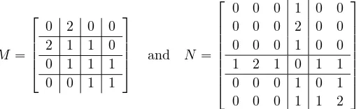
graphH in Figure 1.2(b). It is useful to see how matrices corresponding to a graph and a blowup of the graph are related. OverF3, let
M =
0 2 0 0 2 1 1 0 0 1 1 1 0 0 1 1
and N =
0 0 0 1 0 0 0 0 0 2 0 0 0 0 0 1 0 0 1 2 1 0 1 1 0 0 0 1 0 1 0 0 0 1 1 2
(a) (b)
Fig. 2.1: Graphs in Theorem 2.2
Then M is an example of a matrix corresponding to G and N is an example of a matrix corresponding toH. Note that, for example, the entrym11was replaced with
a 3×3 zero block in N, the entry m12 was replaced with a 3×1 nonzero block in
N, the entries in the last row and column of M were replaced with empty blocks (i.e., erased), and the diagonal entries of N were changed to whatever was desired. These substitutions of block matrices correspond to the vertex substitutions used to constructH.
We will introduce our method by presenting a proof of a special case of a charac-terization theorem from [10] which characterizesG2(F2). We will then generalize this
proof into a characterization of all simple graphs in Gk(Fq) for any k and q. After giving examples for some specifick andq, we will describe the strong connection to projective geometry and list some consequences of this connection.
2. A new approach to a recent result. We will introduce our method by giving a proof of a special case of Theorems 5 and 6 of [10].
Theorem 2.1 ([10]). LetGbe a simple graph onnvertices. Thenmr(F2, G)≤2
if and only if the simple version of Gc is either of the form
(Ks1∪Kp1,q1)∨Kr
for some appropriate nonnegative integerss1,p1,q1, andr, or of the form
(Ks1∪Ks2∪Ks3)∨Kr
for some appropriate nonnegative integerss1,s2, s3, andr.
We first rephrase Theorem 2.1 using blowup graph terminology.
Theorem 2.2 ([10]). LetGbe a simple graph onnvertices. Thenmr(F2, G)≤2
(i.e., G∈ G2(F2)) if and only ifGis a blowup of either of the graphs in Figure 2.1.
Lemma 2.3 ([15, Theorem 8.9.1]). LetAbe ann×nsymmetric matrix of rankk. Then there is an invertible principal k×k submatrix B of A and a k×nmatrix U
such that
A=UtBU.
Corollary 2.4. Let A be an n×n symmetric matrix. Then rankA ≤ k if and only if there is some invertible k×k matrix B and k×n matrix U such that
A=UtBU.
Proof. LetAhave rank r≤k. Then by Lemma 2.3, there is an invertibler×r
matrixB1 and anr×nmatrixU1 such thatA=U1tB1U1. LetB2=
B1 O
O Ik−r
and U2=
U1
O
(whereO represents a zero matrix of the appropriate size). Then
A=Ut
2B2U2. The reverse implication follows from the rank inequality rank(UtBU)≤
rankB.
Recall that two square matricesAandBare congruent if there exists some invert-ible matrixCsuch thatA=CtBC. It is straightforward to show that congruence is an equivalence relation. LetBconsist of one representative from each congruence equiva-lence class of invertible symmetrick×kmatrices. By Corollary 2.4, ifAis a symmetric
n×nmatrix with rankA≤k, thenA∈ {UtBU
| B∈ B, U a k×nmatrix}.
We now proceed with the proof of Theorem 2.2.
Proof. [Proof of Theorem 2.2] First, we compute a suitableB, a set of represen-tatives from the congruence classes of invertible symmetric 2×2 matrices overF2. If
an invertible symmetric 2×2 matrixB over F2 has a nonzero diagonal entry, then
B=
1 1 1 0
,B =
0 1 1 1
, orB=I2. In any of these three cases,BtBB =I2, so
B is congruent to the identity matrix I2. If an invertible symmetric 2×2 matrix B
overF2 has all zeros on the diagonal, then the off-diagonal entries must be nonzero,
soB =
0 1 1 0
. In this case,
a c
b d
0 1 1 0
a b
c d
=
ac+ac ad+bc ad+bc bd+bd
=
0 ad+bc
ad+bc 0
,
so any matrix congruent toB will have a zero diagonal. Therefore, a suitableB is
B=
I2,
0 1 1 0
Because U is a matrix with entries in 2, the columns ofU are members of the finite set 1 0 , 0 1 , 1 1 , 0 0 .
LetAbe a symmetrick×kmatrix. For anyn×npermutation matrixP, the graphs ofAand PtAP are isomorphic. Therefore we may assume that identical columns of
U are contiguous and write U =
E1 E2 J O
where E1 is 2×pmatrix with
each column equal to
1
0
,E2 is 2×qmatrix with each column equal to
0
1
,J
is a 2×rmatrix with each entry equal to 1, andOis a 2×tzero matrix. Then either
A= ET 1 ET 2 JT OT
E1 E2 J O =
Jp O Jp,r O
O Jq Jq,r O
Jr,p Jr,q Or O
O O O Ot
or else A= ET 1
E2T
JT OT 0 1 1 0
E1 E2 J O =
Op Jp,q Jp,r O
Jq,p Oq Jq,r O
Jr,p Jr,q Or O
O O O Ot
,
whereJ is an all-ones matrix, O is a zero matrix, and subscripts ofJ and O denote the dimensions of the matrix.
Any simple graph corresponding to the first matrix is a blowup of the graph in Figure 2.1(a), while any simple graph corresponding to the second matrix is a blowup of the graph in Figure 2.1(b). Thus we have established Theorem 2.2.
Observation 2.5. Note that every block in the above matrices is either a O
matrix or aJ matrix. Consequently, we could have obtained the zero/nonzero form
of the matrices with rank at most 2 by only considering U =
1 0 1 0 0 1 1 0
and
computing
A=UtU =
1 0 1 0 0 1 1 0 1 1 0 0 0 0 0 0
and
A=UtB2U =
1 0 0 1 1 1 0 0
0 1 1 0
1 0 1 0
=
0 1 1 0 1 0 1 0 1 1 0 0 0 0 0 0
[image:7.612.69.433.211.420.2]The nonzero diagonal entries correspond to loops in our graphs. This simplified procedure again yields the graphs in Figure 2.1.
In the proof of Theorem 2.2, we noted that anyU could be written in a standard form. In Observation 2.5, we saw how the standard form ofU could be simplified to take advantage of the theorem being about blowup graphs. We will now discuss the reasoning behind these constructions and show that an analogous standard form of
U exists for any finite field and anyk.
Because we construct the graphs using representatives of congruence classes, it is important for any simplifiedU to have the property that if B and ˆB are congruent, thenUtBU andUtBUˆ correspond to isomorphic graphs. The following lemma shows that if we take a matrix U where the columns consist of all vectors in Fkq, like in
Observation 2.5, and if B and ˆB are congruent, then UtBU and UtBUˆ correspond to isomorphic graphs.
Lemma 2.6. Let U be the matrix with columns {v | v∈ Fkq}. LetB and C be
invertiblek×kmatrices withB symmetric. Then the graphs corresponding toUtBU
andUt(CtBC)U are isomorphic.
Proof. Since every vector inFkqappears as a column ofUand the mappingx7→Cx
is one-to-one, CU is just a column permutation of U. This permutation induces a relabeling of the graphUtBU to give the graph of (CU)tB(CU) =Ut(CtBC)U.
Though this invariance property with respect to congruent matrices does not hold for an arbitraryU, there is another smaller U which does have the same property. We first need some preliminary material. Then we will introduce this new U in Lemma 2.9.
Definition 2.7. LetF be a field. Two nonzero vectorsv1, v2∈Fk are
projec-tively equivalent if there exists some nonzero c∈F such thatv1=cv2.
It is easy to check that projective equivalence is in fact an equivalence relation on the vectors inV.
We pause to note that replacing a column of U with a projectively equivalent column does not affect the graph corresponding to UtBU. To see this, let U = [u1 u2 · · · un] and let i ∈ {1,2, . . . , n}. Let ˆU be the matrix obtained from U by
replacing the column ui with cui for some nonzero c ∈ F. Then the i, j entry of ˆ
UtBUˆ, (cui)tBu
j ifi6=jor (cui)tB(cui) ifi=j, is zero if and only if thei, jentry of
UtBU,utiBuj, is zero. Thus the graphs associated withUtBU and ˆUtBUˆ are equal.
Lemma 2.8. LetF be any field, letx∈Fk, letx¯denote the projective equivalence
class of x, and letP =∪x∈Fk−~0{x¯}, the set of projective equivalence classes in Fk.
bijection.
Proof. The functionf is well-defined since ifCx=y, then for any nonzerok∈F,
C(kx) =kCx=ky= ¯y. IfCx1=Cx2, then for some nonzero k∈F, kCx1=Cx2,
which implies C(kx1−x2) = 0, giving kx1 = x2 since C is invertible. Therefore
x1 =x2 andf is injective. Surjectivity off also follows from the hypothesis that C
is invertible.
Lemma 2.9. Let x1, x2, . . . , xm be the projective equivalence classes of Fkq −~0,
with each xi as a chosen representative from its class. LetU = [x1 x2 · · · xm], the
matrix with column vectorsx1, x2, . . . , xm. LetB andC be invertible k×k matrices
with B symmetric. Then the graphs corresponding to UtBU and Ut(CtBC)U are
isomorphic.
Proof. Let T =CU. Denote theith column of U by ui and the ith column of
T byti. By Lemma 2.8, the sequence of projective equivalence classest1, t2, . . . , tn is just a permutation of the sequenceu1, u2, . . . , un. Form the matrixSin which theith
column,si, isuj ifti=uj, so thatS is a column permutation ofU andsi=ti. Then the graph corresponding to Ut(CtBC)U = (CU)tB(CU) = TtBT is isomorphic to the graph corresponding toStBS by the reasoning preceding Lemma 2.8, which is in turn just a relabeling of the graph corresponding toUtBU.
We now find a standard form for any matrixU, as in our proof of Theorem 2.2. LetU be ak×nmatrix overFq and letB be an invertible symmetrick×kmatrix
overFq. Letx1, x2, . . . , xmbe the projective equivalence classes ofFkq −~0, with each xi as a chosen representative from its class. For each nonzero columnuiofU, replace
ui with the chosen representative ofui. Then permute the columns ofU so that the matrix is of the form ˆU = [X1 X2 · · · Xm O], where each Xi is a block matrix of columns equal to xi and O is a zero block matrix. Note that some of these blocks may be empty. Let Gbe the simple graph corresponding to UtBU and let ˆGbe the simple graph corresponding to ˆUtBUˆ. From our results above,Gis isomorphic to ˆG.
As illustrated in Observation 2.5, we can obtain the zero/nonzero structure of the block matrix ˆUtBUˆ by simply deleting all duplicate columns of ˆU. Deleting these du-plicate columns of ˆU leaves a matrix that can be obtained from ˜U = [x1x2 · · · xm0] by deleting the columns of ˜U corresponding to empty blocks of ˆU. Let ˜G be the (looped) graph corresponding to ˜UtBU˜. Then ˆGis a blowup of ˜G, which implies that
Gis a blowup of ˜G.
Furthermore, letBbe a set consisting of one representative from each congruence class of invertible symmetric k×k matrices and let ˆB be the representative that is congruent to B. Then from Lemma 2.9, the graphs corresponding to ˜UtBU˜ and
˜
There is another simplification we can make. Notice that both graphs displayed in Theorem 2.2 have an isolated nonlooped vertex. This vertex came from the zero column vectors inU and corresponds to the fact that adding any number of isolated vertices to a graph does not change its minimum rank. In any theorem like Theo-rem 2.2, each graph from which we construct blowups will always have this isolated nonlooped vertex and so will be of the formG∪K1. Note that in constructing such
a graphG, it is enough to assume that ˜U in the above paragraphs does not have a zero column vector.
Definition 2.10. Let x1, x2, . . . , xm be the projective equivalence classes of
Fkq−~0, with eachxias a chosen representative from its class. LetBbe a set consisting
of one representative from each congruence class of invertible symmetrick×kmatrices. LetU = [x1x2 · · · xm], the matrix with column vectorsx1, x2, . . . , xm. We define the
set of graphsgk(Fq) as the set of graphs corresponding to the matrices in{UtBU |
B∈ B}.
We now have the following result (recall thatK1has no loop).
Theorem 2.11. A simple graph Gis in Gk(Fq) if and only if G is a blowup of
some graph in{H∪K1 | H ∈gk(Fq)}.
Proof. LetG be a simple graph in Gk(Fq). Let A∈ S(Fq, G) be a matrix with rankA≤k. ThenA=UtBU for somek×nmatrixU and some invertible symmetric
k×kmatrixB. Using the procedure outlined in the paragraphs following Lemma 2.9, we see thatGis a blowup of a graph ˜Gcorresponding to ˜UtBU˜, where ˜U andB are defined as in the procedure. Lemma 2.9 then shows that ˜G∈gk(Fq).
Conversely, letGbe a blowup of some graph in{H∪K1 | H ∈gk(Fq)}obtained by replacing each vertexvi of H with a set of vertices Vi and K1 with any number
of vertices. Deleting isolated vertices ofGdoes not change the minimum rank of G, so without loss of generality, we will assume thatG has no isolated vertices (which implies thatK1was replaced with an empty set of vertices). Letx1, x2, . . . , xmbe the projective equivalence classes ofFkq −~0, with eachxias a chosen representative from
its class. Let ˜U = [x1x2 · · · xm] and letB be an invertible symmetrick×kmatrix
such that ˜UtBU˜ corresponds to the graphH. Form the matrix ˆU = [X
1X2 · · · Xm]
by replacing each columnxi of ˜U with the blockXi, where the columns ofXiconsist of |Vi| copies ofxi. Then ˆUtBUˆ corresponds to Gand rank ˆUtBUˆ ≤ksince B has rankk. Thus mr(Fq, G)≤k, soG∈ Gk(Fq).
3. Congruence classes of symmetric matrices over finite fields. Sym-metric matrices represent symSym-metric bilinear forms and play an important role in projective geometry. Two congruent symmetric matrices represent the same sym-metric bilinear form with respect to different bases. Because of their fundamental importance, congruence classes of symmetric matrices over finite fields have been studied and characterized for a long time in projective geometry. In this section, we have distilled the pertinent proofs of these characterizations from [1], [23], and [16] to give a suitable Bfor invertible symmetrick×k matrices overFq for anykandq.
In the next section, we will expound more on the connection between the minimum rank problem and projective geometry.
We need the following elementary lemma.
Lemma 3.1. If a symmetric matrix B =
C D
Dt E
, where C is a square
invertible matrix, then B is congruent to
C O
O E′
, where O is a zero matrix and
E′
is a square symmetric matrix of the same order as E.
Proof. LetR=C−1Dso thatCR=D. Then
I O
−Rt I
C D
Dt E
I −R
O I
=
C D
−RtC+Dt
−RtD+E
I −R
O I
=
C −CR+D
−RtC+Dt RtCR−DtR−RtD+E
=
C O
O E−DtR
,
since−CR+D=O= (−CR+D)t=
−RtC+Dt.
Lemma 3.2. Every symmetric matrix over Fq is congruent to a matrix of the
form diag(a1, a2, . . . , as, b1H1, b2H2, . . . , btHt), where ai, bi ∈ Fq, Hi =
0 1
1 0
,
andsandt are nonnegative integers.
Proof. IfB is the zero matrix, then the result is true.
IfB is not the zero matrix, then the diagonal ofBhas a nonzero entry or there is
someaij6= 0,i6=j, so that B has a principal submatrix of the form
0 a
ij
aij 0
=
aijH, whereH =
0 1 1 0
.
In the first case, by using a suitable permutation, we may assume that b11 6= 0.
In the second case, again by using a suitable permutation, we may assume that the upper left 2×2 principal submatrix isaijH. By Lemma 3.1,B is congruent to diag(aijH, B′).
Continue this process inductively withB′. Then, again using a suitable permu-tation,B is congruent to diag(a1, a2, . . . , as, b1H, b2H, . . . , btH).
We will now treat the even characteristic and odd characteristic cases separately.
3.1. Even characteristic. We first consider the case whenFq has even
charac-teristic. First, we need a well-known result.
Lemma 3.3. Every element in a field of characteristic 2 is a square.
Corollary 3.4. Every symmetric matrix is congruent todiag(Is, H1, H2, . . . , Ht).
Proof. By Lemma 3.2, a symmetric matrixA is congruent to a matrix
B= diag(a1, a2, . . . , as, b1H1, b2H2, . . . , btHt). Let
C= diag(√1
a1,
1 √a
2, . . . ,
1 √a
s, 1 √
b1
I2,
1 √
b2
I2, . . . ,
1 √
bt
I2).
ThenCtBC= diag(I
s, H1, H2, . . . , Ht).
Let B be a symmetric matrix in Fq. Then according to Corollary 3.4, B is
congruent to a matrixC = diag(Is, H1, H2, . . . , Ht), where each Hi =0110. Either
s= 0 ors >0. Ifs >0, then diag(Is, H1, H2, . . . , Ht), and thusB, is congruent to
Ik. To see this, let
A= diag(1, H) =
1 0 0 0 0 1 0 1 0
and C=
1 1 1 1 0 1 0 1 1
.
Then, since charFq= 2,
Ct(AC) =
1 1 0 1 0 1 1 1 1
1 1 1 0 1 1 1 0 1
=I3.
If s = 0, then diag(H1, H2, . . . , Ht) and B have even order and B is congruent to
diag(H1, . . . , Hk/2).
Lemma 3.5. If a symmetric matrix B has a zero diagonal, then every matrix congruent toB has a zero diagonal.
LetB be a symmetric matrix having a zero diagonal. Ifv is thekth column of a matrixC, then the (k, k) entry ofCtBC isvtBv, which is zero, since
vtBv=X i,j
bijvivj=
X
i
biivi2+
X
i<j
bij(vivj+vivj) =
X
i
biivi2= 0.
The results in this subsection give us the following lemma.
Lemma 3.6. Let q be even. To determine gk(Fq), we may take B as follows: if
k is odd, then B ={Ik}; if k is even, then B ={Ik,diag(H1, H2, . . . , Hk/2)}, where
Hi =
0 1 1 0
.
3.2. Odd characteristic. We now consider the case when Fq has odd
charac-teristic. We first need a well-known result.
Lemma 3.7. If Fq has odd characteristic and ν∈Fq, then there existsc, d∈Fq
such that c2+d2=ν.
Proof. LetA={c2
| c∈Fq}andB={ν−d2 | d∈Fq}. Since the mapσ:F× q →
F×q given by σ:x7→ x2 has kernel {1,−1}, there are (q−1)/2 squares in Fq \ {0}.
Including zero, there are then (q+ 1)/2 squares inFq. Thus|A|=|B|= (q+ 1)/2, so A∩B6=∅, andc2=ν
−d2 for somec, d
∈Fq.
Since there are (q−1)/2 nonzero squares inFq, given a nonsquare ν ∈Fq, the
set {νb2 | b∈F
q, b6= 0}is a set of (q−1)/2 nonsquares in Fq. Consequently, every nonsquare is equal toνb2for some b
∈Fq.
The matrixaH for anya∈Fq is congruent to a diagonal matrix:
1 1 −1 1
0 a
a 0
1 −1 1 1
=
a a
a −a
1 −1 1 1
=
2a 0 0 −2a
.
This fact combined with Lemma 3.2 shows that every symmetric matrix over Fq is
congruent to a diagonal matrix.
Lemma 3.8. Every invertible symmetrick×kmatrixB overFq is congruent to
either Ik ordiag(Ik−1, ν), whereν is any nonsquare in Fq.
LetCbe an invertible diagonal matrix congruent toB, withC=NtBN, and let
ν be any nonsquare inFq.
By a permutation matrixP, letD=PtCP = diag(b2
where the firstselements of the diagonal ofDare squares in qand the lasttelements are nonsquares inFq.
LetQ= diag(b−11, b
−1 2 , . . . , b
−1
s , c −1 1 , c
−1 2 , . . . , c
−1
t ). LetE=QtDQ= diag(Is, νIt).
Letc, d∈Fq such thatc2+d2=ν. Let R=ν−1
c d
−d c
.
Since detR=ν−2(c2+d2) =ν−1
6
= 0,R is invertible. Note that
Rt(νI2)R=νRtR=νν−2(c2+d2)I2=I2.
Iftis even, letS= diag(Is, R1, R2, . . . , Rt/2), whereRi=Rfor eachi. ThenStES=
Ik. Iftis odd, letS= diag(Is, R1, R2, . . . , R(t−1)/2,1). ThenStES= diag(Ik−1, ν) .
The next lemma shows that these two cases are in fact different and gives a simple criteria to determine which congruence class any symmetric matrix is in.
Lemma 3.9. If detB is a square (nonsquare) and Bˆ is congruent to B, then
det ˆB is a square (nonsquare).
Proof. Let ˆB=CtBC. Then det ˆB= (detC)2(detB). Thus detB is a square if
and only if det ˆB is a square.
Since detIk = 1 is a square and det(diag(Ik−1, ν)) = ν is a nonsquare, we can
determine if a matrix is congruent toIk or congruent to diag(Ik−1, ν) by whether the
determinant is a square or not.
It appears then that |B| = 2. However, we can do better in one case since we only are concerned with whether an entry of UtBU is zero or nonzero and not with the actual value of the entry.
Definition 3.10. LetB and ˆB be matrices. If ˆB =dCtBC for some invertible matrixCand some nonzero constantd, thenB and ˆB areprojectively congruent.
Since multiplying by a nonzero constant preserves the zero/nonzero pattern in a matrix over a field, if B and ˆB are projectively congruent, then UtBU and UtBUˆ give isomorphic graphs.
Lemma 3.11. Ifkis odd, then an invertible symmetrick×kmatrix is projectively congruent toIk.
Proof. Letk= 2ℓ−1. We can see that det(νdiag(Ik−1, ν)) =ν2ℓ−1ν =ν2ℓ is a
square. Thus diag(Ik−1, ν) is projectively congruent toIk.
4 5
3 1 2
7 6
(a)F2R3
1 2 3 4 5
6
7
8
9
10 11 12
13
[image:15.612.82.431.148.311.2](b)F3R3
Fig. 3.1: Graphs in Corollaries 3.14 and 3.15
Lemma 3.12. Let q be odd. To determine gk(Fq), we may take B as follows: if
k is odd, then B = {Ik}; if k is even, then B ={Ik,diag(Ik−1, ν)}, where ν is any
nonsquare inFq.
3.3. Summary. Combining Lemmas 3.6 and 3.12, the results of this section can be summarized as the following theorem.
Theorem 3.13. The setgk(Fq) is the set of graphs of the matrices in{UtBU |
B∈ B}, where the columns ofU are a maximal set of nonzero vectors inFkq such that
no vector is a multiple of another andB is given by:
1. if kis odd,B={Ik}.
2. if k is even and charFq = 2,B ={Ik,diag(H1, H2, . . . , Hk/2)}, where Hi = 0 1
1 0
.
3. if k is even and charFq 6= 2, B = {Ik,diag(Ik−1, ν)}, where ν is any
non-square in Fq.
3.4. Examples of characterizations. As special cases of Theorem 3.13, we present the following corollaries which calculate gk(Fq) for several k and q. In the corollaries, we label a graph ingk(Fq) using the patternF qRk, signifying that it is a graph for the mr(Fq, G)≤kcorollary. To compute these graphs, we used the software
program Sage [32] and the Sage functions listed in Appendix A.
In these theorems, recall thatK1 does not have a loop.
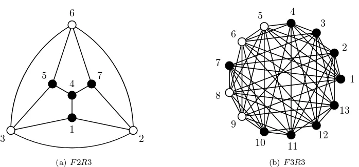
Fig-ure 3.1(a). Thenmr( 2, G)≤3(i.e., G∈ G3( 2)) if and only ifGis a blowup graph
of F2R3∪K1.
As matrices overF2, let
U =
0 1 0 1 0 1 1 0 0 1 1 1 1 0 1 1 1 1 0 0 0
and B=
1 0 0 0 1 0 0 0 1
.
Then the graphF2R3 corresponds to the matrix
UtBU =
1 1 1 1 0 0 0 1 0 1 0 0 1 1 1 1 0 0 1 1 0 1 0 0 1 1 0 1 0 0 1 1 1 1 0 0 1 1 0 1 0 1 0 1 0 1 0 1 1
.
Similarly, straightfoward matrix calculations give the following corollaries.
Corollary 3.15. Let G be any simple graph. Let F3R3 be the graph in Fig-ure 3.1(b). Then mr(F3, G)≤3 (i.e.,G∈ G3(F3)) if and only if Gis a blowup graph
of F3R3∪K1.
The next corollary gives the simplest previously-unknown result for whichgk(Fq) contains two graphs.
Corollary 3.16. Let Gbe any simple graph. Let F2R4A and F2R4B be the graphs in Figure 3.2. Then mr(F2, G)≤ 4 (i.e., G ∈ G4(F2)) if and only if G is a
blowup graph of eitherF2R4A∪K1 orF2R4B∪K1.
4. Connection to projective geometry. As mentioned previously, the clas-sifications of symmetric matrices in Section 3 are standard classification results in projective geometry. In this section, we first review appropriate terminology and highlight this connection to projective geometry. We will define slightly more ter-minology than is strictly necessary to help the reader see where these things fit into standard projective geometry. We then give some examples of how results in projec-tive geometry can help us understandgk(Fq) better. For further material, a definitive treatise on projective geometry is contained in the series [23] and [24].
1 2 3 4 5 6
7
8
9
10
11
12 13 14
15
(a)F2R4A
1 2 3 4 5 6
7
8
9
10
11
12 13 14
15
[image:17.612.82.429.151.318.2](b)F2R4B
Fig. 3.2: Graphs in Corollary 3.16
Definition 4.1. Let V =Fnq+1, the vector space of dimension n+ 1 over Fq.
Forx, y∈V −~0, we define an equivalence relation by
x∼y ⇐⇒ x=cy, wherec∈Fqandc6= 0.
Denote the equivalence class containing x∈ V −~0 as ¯x= {cx | c ∈Fqandc 6= 0}.
Geometrically, we can think of the class ¯xas the set of non-origin points on a line passing throughxand the origin inV. These equivalence classes form theprojective geometry P G(n, q) of (projective) dimensionnand orderq. The equivalence classes are called thepointsofP G(n, q). Each subspace of dimensionm+ 1 inV corresponds to a subspace of (projective) dimensionmin P G(n, q). If a projective geometry has (projective) dimension 2, then it is called aprojective plane.
Note that there is a shift by one in dimension between a vector spaceV and its subspaces and the projective geometry associated with V and its subspaces. To help the reader, we will use the nonstandard termprojective dimension (or “pdim”) when dealing with the dimension of a projective geometry.
Definition 4.2. Let S be the set of subspaces of P G(n, q). A correlation
σ: S → S is a bijective map such that for any subspaces R, T ∈ S, R ⊆T implies that σ(T)⊆σ(R) and pdimσ(R) =n−1−pdimR. Apolarity is a correlationσ of order 2 (i.e., σ2= 1, the identity map).
Note that any polarityσmaps points inSto hyperplanes (subspaces of projective dimensionn−1 inS) and hyperplanes to points. Sinceσ2= 1, we haveY =σ(¯x) if
Definition 4.3. Letσbe a polarity onP G(n, q). Let ¯x,y¯be points inP G(n, q). We say thatσ(¯x) is thepolar (hyperplane) of ¯xand ¯xis thepole ofσ(¯x). If ¯y∈σ(¯x), then ¯x∈σ(¯y) and we say that ¯xand ¯yareconjugate points. If ¯x∈σ(¯x), then we say that ¯xis self-conjugate orabsolute. Similarly, ifS is a subspace ofP G(n, q), then S
is absolute if σ(S)⊆S orS ⊆σ(S). A subspace of P G(n, q) consisting of absolute points is calledisotropic.
The next definition gives the connection with symmetric matrices.
Definition 4.4. LetB be an (n+ 1)×(n+ 1) invertible symmetric matrix over
Fq. Defineσ:S → S byσ:R7→R⊥, where the orthogonality relation is defined by
the nondegenerate symmetric bilinear form represented byB(i.e.,R⊥ =
{y¯ | xtBy= 0forall¯x∈R}). We callσthe polarity associated withB.
The fact that theσin the previous definition is a polarity is easy to check.
LetM1andM2be symmetric matrices. Letσ1andσ2be the associated polarities,
respectively. Two polarities are equivalent if the matrices are projectively congruent, i.e.,σ1 is equivalent toσ2 ifM1=dCtM2C for some nonzerodand invertible matrix
C. Thus there is a unique polarity associated with each matrix given in Theorem 3.13.
We now summarize from [23, Section 2.1.5] the classification of polarities that are associated with symmetric matrices. Let B be an invertible symmetric matrix over
Fq. Letσbe the polarity associated with B.
• Ifqis odd, thenσis called anordinary polarity.
IfBhas even order, then the associated polarity is either ahyperbolicpolarity or anelliptic polarity. The correspondence between these types of polarities and the matrices in B from Theorem 3.13(3) is slightly nontrivial and is summarized in [23, Corollary 5.19].
IfB has odd order, thenσis a parabolic polarity, which corresponds toBin Theorem 3.13(1).
• If q is even andbii = 0 for all i, then σ is a null polarity (or in alternate terminology,σis asymplectic polarity). Note that this only occurs when B
has even order since otherwiseB is not invertible. This case corresponds to the non-identity matrix in theBin Theorem 3.13(2).
• Ifq is even and there is somebii 6= 0, thenσ is apseudo-polarity. This case corresponds to the identity matrix inB in Theorem 3.13(1) or (2).
We now examine the connection to graphs by recalling the definition of a polarity graph.
Definition 4.5. LetB be an invertible symmetric (n+ 1)×(n+ 1) matrix over
Fq and letσ be the associated polarity. The polarity graph of σ has as its vertices
the points of P G(n, q) and as its edges {x¯¯y | xtBy = 0
}. In a polarity graph, ¯x
is adjacent to ¯y exactly when ¯x and ¯y are conjugate (i.e., x and y are orthogonal with respect to B). In standard literature, loops are not allowed in polarity graphs. However, for our purposes, loops convey needed information, so a vertex ¯xin a polarity graph has a loop if and only if ¯xis absolute (i.e.,xtBx= 0, whereB is an invertible symmetric matrix associated with the polarity).
In Theorem 3.13, the vertices of a graph in gk(Fq) represent the points of the
projective geometryP G(k−1, q) and an edge is drawn if the corresponding points are not conjugate (i.e., xtBy 6= 0). Thus, the graphs in Theorem 3.13 are exactly the complements of polarity graphs. Recall that when dealing with looped graphs, a vertex is looped in the complement of a graph if and only if it is nonlooped in the original graph.
Using this connection, we can restate Theorem 3.13:
Theorem 4.6. The setgk(Fq)is the set of complements of the (looped) polarity
graphs of the polarities onP G(k−1, q)that are associated with symmetric matrices.
4.2. Consequences of the connection. With the main theorem stated as in Theorem 4.6, we can use a variety of known results about polarity graphs to derive results about graphs in gk(Fq). In this section, we list a few consequences of Theorem 4.6.
An elementary result in projective geometry gives us the size of the graphs in
gk(Fq). While this result could have been realized from the statement in
Theo-rem 3.13, it also naturally follows as a consequence of TheoTheo-rem 4.6.
Theorem 4.7. Every graph in gk(Fq)has q
k−1
q−1 vertices.
Proof. There areqk
−1 vectors inFkq−~0. Since there areq−1 nonzero constants
inFq, there areq−1 elements in each equivalence class inP G(k−1, q), so there are
qk−1
q−1 points in P G(k−1, q).
The following observation follows directly from Theorem 4.6 and restates the criteria for an edge in a graph ingk(Fq) in several ways.
1. uBv6= 0 (equivalently,v Bu6= 0), or equivalently, 2. uand vare not conjugate points, or equivalently, 3. u6∈σ(v) (equivalently,v6∈σ(u)).
Corollary 4.9. A graph G∈gk(Fq) is regular of degree qk−1 (using the
con-vention that a loop adds one to the degree of a vertex). Letv ∈Gand letσbe the polarity associated withG. Since the hyperplaneσ(v) contains qk−q−11−1 points, this is the degree of avin the complement ofG. Thus the degree ofv inGis
qk −1
q−1 −
qk−1
−1
q−1 =q
k−1.
In light of Observation 4.8, determining the numbers of looped and nonlooped vertices inGis equivalent to finding the numbers of absolute points of the polarities ofP G(k−1, q).
Theorem 4.10. Let Fq be a finite field having characteristic 2. One graph in
gk(Fq)will have q
k−1−1
q−1 nonlooped vertices. If kis even, then the additional graph in
gk(Fq) will have all nonlooped vertices.
Proof. In a field of characteristic 2, since
xtBx=X i,j
bijxixj =
X
i
biix2i +
X
i<j
bij(xixj+xixj) =
X
i
biix2i =
X
i
p biixi
!2 ,
a point ¯xis absolute if and only ifP
i √b
iixi= 0.
In a pseudo-polarity, the set of absolute points is the hyperplaneP
i √
biixi= 0. Since a hyperplane ofP G(k−1, q) is a projective geometry of projective dimension
k−2, there are qk−q−11−1 nonlooped vertices in this graph.
In a null polarity,bii= 0 for alli. Therefore every vertex is nonlooped (i.e., there are qk−1
q−1 nonlooped vertices). A null polarity occurs whenkis even.
For the odd characteristic case, we will directly apply a standard result in pro-jective geometry about the number of absolute points in ordinary polarities.
Theorem 4.11 ([24, Theorem 22.5.1(b)]). Let q be odd. Then the number of absolute points in a polarity inP G(k−1, q) is given by:
• (qm−1)(q−qm−1 1+1) or
(qm+1)(qm−1−
1)
q−1 ifk= 2mis even;
• q2m−1
q−1 if k= 2m+ 1 is odd.
Corollary 4.12. Let q be odd. If k = 2m is even, then the two graphs in gk(Fq) will have (q
m−1)(qm−1
+1)
q−1 and
(qm+1)(qm−1−
1)
q−1 nonlooped vertices, respectively.
If k= 2m+ 1 is odd, then the graph ingk(Fq)will have q 2m−1
We conclude by applying a few standard results for polarities over P G(2, q) (a projective plane) to give results about g3(Fq) and the minimum rank problem. We note that the polarity graphs ofP G(2, q) for anyqare the Erd˝os-R´enyi graphs from extremal graph theory (see [19], [20], or [12]). For a survey of interesting properties of the Erd˝os-R´enyi graphs and their subgraphs, see [30] or [34, Chapter 3].
Theorem 4.13. IfG∈g3(Fq), then the nonlooped vertices inGform a clique.
Proof. Suppose that uand v are distinct nonadjacent nonlooped vertices in G. Thenuandvare absolute vertices and u∈σ(u)∩σ(v) andv∈σ(u)∩σ(v). This is a contradiction since the intersection of any two distinct lines inP G(2, q) is a single point.
IfG∈g3(Fq), the formulas in Theorem 4.10 and Corollary 4.12 imply thatGhas
q+ 1 nonlooped vertices. This combined with Corollary 4.9 and Theorem 4.13 gives the following corollary.
Corollary 4.14. If G ∈ g3(Fq), then each nonlooped vertex is adjacent to q
nonlooped vertices and q2−q looped vertices.
Theorem 4.13 also gives us the following theorem.
Theorem 4.15. Let G=Ks1,s2,...,sn, a simple complete multipartite graph. If q≥n−1, thenmr(Fq, G)≤3.
Proof. LetG=Ks1,s2,...,sn. ThenGis a blowup graph ofKn, where each vertex
of Kn is nonlooped. Since the graph ing3(Fq) contains a clique ofq+ 1 nonlooped vertices, ifq+ 1≥n, thenGis a blowup graph of the graph ing3(Fq).
We can now construct an interesting family of simple graphs.
Theorem 4.16. For every integern≥1, letGnbe a simple complete multipartite
graph H1∨H2∨ · · · ∨Hn where each Hi is an independent set with si > (n−1)2
vertices. We then have mr(Fq, Gn)≤3 if and only ifq≥n−1.
Proof. Ifq≥n−1, then mr(Fq, Gn)≤3 by Theorem 4.15.
Conversely, letq < n−1. LetI be the graph in g3(Fq) and letI1 andI2 be the
subgraphs ofIinduced by the looped and nonlooped vertices ofI, respectively. Since
I1 hasq2 vertices, any blowup ofI1 containing more thanq2 vertices will contain an
edge by the pigeon-hole principle. Since the vertices in eachHiform an independent set of sizesi >(n−1)2 > q2, at least one vertex in each Hi must be a blowup of a vertex inI2. Furthermore, since the vertices of eachHi have the same neighbors, we can assume without loss of generality that all of the vertices of eachHi are blowups of vertices ofI1. ThusGn is a blowup ofI2. However, any blowup of I2 will be of
sinceq+ 1< n.
5. Conclusion. We have suceeded in classifying the structure of graphs inGk(Fq)
for anykand anyq. We have also shown how this classification relates to projective geometry. We have applied a few results of projective geometry to give results in the minimum rank problem.
We conclude with a short list of open questions and topics for further investiga-tion. First, there are many results about polarity graphs that could potentially yield results for the minimum rank problem. What other facts from projective geometry can be applied to give results in the minimum rank problem over finite fields?
The structural characterization in this paper gives rise to a theoretical procedure for determining the minimum rank of any graph over a finite field. How can this procedure be efficiently implemented? How can the results of Ding and Kotlov [18] be combined with the classification in this paper to yield results on minimal forbidden subgraphs describingGk(Fq)? The author has implemented such an algorithm and has
some preliminary results on the numbers of forbidden subgraphs describing Gk(Fq)
for different values ofk andq.
Finally, there is still ongoing research investigating the structure of polarity graphs. For example, Jason Williford [34], Michael Newman, and Chris Godsil [21] have recently investigated the sizes of independent sets in polarity graphs. Are there results in the minimum rank problem that would aid in answering questions about the structure of polarity graphs?
Acknowledgment. The author thanks Wayne Barrett and Don March for work in the early part of this research, including the proof of Theorem 2.2 and early com-putational experiments, as well as Willem Haemers for pointing out that the graph
F2R3 is related to the Fano projective plane, which led to the investigation of the connection to projective geometry. Most of this research was done for the author’s Ph.D. dissertation and the support of Brigham Young University is gratefully ac-knowledged. Additionally, the support of Iowa State University during the editing phase is gratefully acknowledged.
REFERENCES
[1] A. Adrian Albert. Symmetric and alternate matrices in an arbitrary field. I. Trans. Amer. Math. Soc., 43(3):386–436, 1938.
[3] Efrat Bank. Symmetric matrices with a given graph. Master’s thesis, Technion–Israel Institute of Technology, February 2007.
[4] Francesco Barioli and Shaun Fallat. On the minimum rank of the join of graphs and decom-posable graphs.Linear Algebra Appl., 421(2-3):252–263, 2007.
[5] Francesco Barioli, Shaun Fallat, and Leslie Hogben. Computation of minimal rank and path cover number for certain graphs.Linear Algebra Appl., 392:289–303, 2004.
[6] Francesco Barioli, Shaun Fallat, and Leslie Hogben. On the difference between the maximum multiplicity and path cover number for tree-like graphs.Linear Algebra Appl., 409:13–31, 2005.
[7] Francesco Barioli, Shaun Fallat, and Leslie Hogben. A variant on the graph parameters of Colin de Verdi`ere: implications to the minimum rank of graphs. Electron. J. Linear Algebra, 13:387–404 (electronic), 2005.
[8] Wayne Barrett, Jason Grout, and Raphael Loewy. The minimum rank problem over the finite field of order 2: Minimum rank 3. Linear Algebra and its Applications, 430(4):890 – 923, 2009.
[9] Wayne Barrett, Hein van der Holst, and Raphael Loewy. Graphs whose minimal rank is two. Electron. J. Linear Algebra, 11:258–280 (electronic), 2004.
[10] Wayne Barrett, Hein van der Holst, and Raphael Loewy. Graphs whose minimal rank is two: the finite fields case.Electron. J. Linear Algebra, 14:32–42 (electronic), 2005.
[11] Am´erico Bento and Ant´onio Leal Duarte. On Fiedler’s characterization of tridiagonal matrices over arbitrary fields.Linear Algebra Appl., 401:467–481, 2005.
[12] W. G. Brown. On graphs that do not contain a Thomsen graph.Canad. Math. Bull., 9:281–285, 1966.
[13] Guantao Chen, Frank J. Hall, Zhongshan Li, and Bing Wei. On ranks of matrices associated with trees.Graphs Combin., 19(3):323–334, 2003.
[14] Nathan L. Chenette, Sean V. Droms, Leslie Hogben, Rana Mikkelson, and Olga Pryporova. Minimum rank of a tree over an arbitrary field. Electron. J. Linear Algebra, 16:183–186 (electronic), 2007.
[15] Gordon Royle Chris Godsil. Algebraic Graph Theory. Springer-Verlag, 2001.
[16] P. M. Cohn. Basic algebra. Springer-Verlag London Ltd., London, 2003. Groups, rings and fields.
[17] Yves Colin de Verdi`ere. Multiplicities of eigenvalues and tree-width of graphs. J. Combin. Theory Ser. B, 74(2):121–146, 1998.
[18] Guoli Ding and Andre˘ı Kotlov. On minimal rank over finite fields.Electron. J. Linear Algebra, 15:210–214 (electronic), 2006.
[19] P. Erd˝os and A. R´enyi. On a problem in the theory of graphs.Magyar Tud. Akad. Mat. Kutat´o Int. K¨ozl., 7:623–641 (1963), 1962.
[20] P. Erd˝os, A. R´enyi, and V. T. S´os. On a problem of graph theory.Studia Sci. Math. Hungar., 1:215–235, 1966.
[21] C D Godsil and M W Newman. Eigenvalue bounds for independent sets, 2005.
[22] Frank J. Hall, Zhongshan Li, and Bhaskara Rao. From Boolean to sign pattern matrices.Linear Algebra Appl., 393:233–251, 2004.
[23] J. W. P. Hirschfeld.Projective geometries over finite fields. Oxford Mathematical Monographs. The Clarendon Press Oxford University Press, New York, second edition, 1998.
[24] J. W. P. Hirschfeld and J. A. Thas. General Galois geometries. Oxford Mathematical Mono-graphs. The Clarendon Press Oxford University Press, New York, 1991. , Oxford Science Publications.
[25] Liang-Yu Hsieh. On Minimum Rank Matrices having a Prescribed Graph. PhD thesis, Uni-versity of Wisconsin, Madison, 2001.
factors.
[27] Charles R. Johnson and Carlos M. Saiago. Estimation of the maximum multiplicity of an eigenvalue in terms of the vertex degrees of the graph of a matrix. Electron. J. Linear Algebra, 9:27–31 (electronic), 2002.
[28] J´anos Koml´os, G´abor N. S´ark¨ozy, and Endre Szemer´edi. Blow-up lemma. Combinatorica, 17(1):109–123, 1997.
[29] Peter M. Nylen. Minimum-rank matrices with prescribed graph.Linear Algebra Appl., 248:303– 316, 1996.
[30] T. D. Parsons. Graphs from projective planes. Aequationes Math., 14(1-2):167–189, 1976. [31] John Sinkovic. The relationship between the minimal rank of a tree and the rank-spreads of
the vertices and edges. Master’s thesis, Brigham Young University, December 2006. [32] William Stein. Sage Mathematics Software (Version 2.8.15). The Sage Group, 2007. http:
//www.sagemath.org.
[33] Hein van der Holst. Graphs whose positive semi-definite matrices have nullity at most two. Linear Algebra Appl., 375:1–11, 2003.
[34] Jason Williford. Constructions in finite geometry with applications to graphs. PhD thesis, University of Delaware, 2004.
Appendix A. Sage code to generate graphs.
# This code i s w r i t t e n f o r Sage 2 . 8 . 1 5 . # See h t t p : / /www. sagemath . org /
def b i l i n e a r f o r m s (F , mr ) :
5 # C o n s t r u c t a m a t r i x s p a c e f o r our b i l i n e a r forms MSpace = Ma tr ixSpa ce (F , mr )
# The i d e n t i t y m a t r i x i s a l w a y s # a con gru en ce c l a s s r e p r e s e n t a t i v e
fo r ms = [ MSpace . i d e n t i t y m a t r i x ( ) ]
10 # Add t h e e x t r a m a t r i c e s i n t h e even rank c a s e s
i f(mod(mr ,2 )= = 0 ): # even rank
i f(F . c h a r a c t e r i s t i c ()==2): # c h a r a c t e r i s t i c 2 # Add diag(H1, H2, . . . , Hmr/2)
h y p e r b o l i c = ma tr ix (F , [ [ 0 , 1 ] , [ 1 , 0 ] ] )
15 h y p e r b o l i c f o r m = ma tr ix (F , [ ] )
f o r i i n ( 1 . . I n t e g e r (mr / 2 ) ) :
h y p e r b o l i c f o r m = h y p e r b o l i c f o r m\
. blo ck sum ( h y p e r b o l i c ) fo r ms . append ( h y p e r b o l i c f o r m )
20 e l s e: # odd c h a r a c t e r i s t i c
# Add diag(In−1, ν), where ν i s a non−s q u a r e
n o n i d e n t i t y f o r m = MSpace . i d e n t i t y m a t r i x ( )
# Find a non−s q u a r e
f o r nu i n F :
break i f nu . i s s q u a r e ( ) :
r a i s e NotImplementedError , \
” Cannot f i n d a non−s q u a r e i n f i e l d . ”
30 n o n i d e n t i t y f o r m [ mr−1 , mr−1] = nu fo r ms . append ( n o n i d e n t i t y f o r m )
return fo r ms
def g e t m a t r i c e s (F , mr ) :
35 # U has one v e c t o r f o r e v e r y e q u i v a l e n c e c l a s s
# i n P G(mr−1, q) U = ma tr ix (F , [ l i s t ( v )
f o r v i n P r o j e c t i v e S p a c e (mr−1 ,F ) ] )\ . t r a n s p o s e ( )
40 B = b i l i n e a r f o r m s (F , mr )
return U, B
def g e t g r a p h s (F , mr ) :
U, B = g e t m a t r i c e s (F , mr )
45 p r o d u c t m a t r i c e s = [U. t r a n s p o s e ( )∗b∗U f o r b i n B ] g r a phs = [ Graph (m) f o r m i n p r o d u c t m a t r i c e s ]
f o r i i n r a ng e ( l e n ( g r a phs ) ) : g r a phs [ i ] . l o o p s ( t r u e ) ;
g r a phs [ i ] . a d d e d g e s ( [ [ j , j ] f o r j
50 i n r a ng e ( l e n ( g r a phs [ i ] ) ) \
i f p r o d u c t m a t r i c e s [ i ] [ j , j ] != 0 ] )
return g r a phs
55 def sho w g r a phs (F , mr ) :
f o r g i n g e t g r a p h s (F , mr ) :
# V e r t i c e s w i t h l o o p s are b l a c k , o t h e r s are w h i t e
v c o l o r s={’ b l a c k ’ : g . l o o p v e r t i c e s ( ) ,\ ’ white ’ : [ i f o r i i n g . v e r t i c e s ( )
60 i f i not i n g . l o o p v e r t i c e s ( ) ]}
g . show ( l a y o u t= ’ c i r c u l a r ’ , v e r t e x c o l o r s=v c o l o r s , \ v e r t e x l a b e l s= f a l s e )
# To r e t r i e v e t h e m a t r i c e s f o r g r a p h s i n g3(F2):
# To r e t r i e v e t h e g r a p h s i n g3( 2):
g r a p h l i s t = g e t g r a p h s (F=F i n i t e F i e l d ( 2 ) , mr=3)