IMPACT EVALUATION OF THE SCHOOL OPERATIONAL ASSISTANCE
PROGRAM (BOS) USING THE MATCHING METHOD
Eny Sulistyaningrum
Faculty of Economics and Business Universitas Gadjah Mada
ABSTRACT
Investment in human capital, especially in children’s education, is considered to be among the most effective ways for countries to improve their national welfare and reduce poverty in the long term. The Government of Indonesia has promoted human capital investment, especially in children, by designing school subsidy programs. Since 2005, the school operational assistance program (BOS) has been the biggest school subsidy program in Indonesia during the last two decades. This paper evaluates the impact of BOS on children’s test scores at the early stage. This study uses Propensity Score Matching (PSM) to estimate the average treatment effect, in the absence of selection, on unobserved characteristics. The results confirm that BOS can increase student performance. The finding suggests that the Government of Indonesia needs to develop a subsidy program to provide a basic level of education for all students, especially for the poor, as the recent school subsidy program is only sufficient for school fees or even only enough for tuition fees if the students live in urban areas. The remainder of the education expenditures must be covered by the household.
Keywords: school subsidy, BOS, PSM, test scores JEL: H52, I22, I25
INTRODUCTION
Investment in human capital, especially in children’s education, is considered to be among the most effective ways for countries to improve their national welfare and reduce poverty in the long term. Becker (1964) pointed out that investment in human capital raises earnings in later life. Undoubtedly, promoting educational attainment can raise living standards on average and contribute to a reduction in absolute poverty by enabling individuals to generate income and access better-paid jobs. Many governments in developing countries have made this one of their top national priorities by ensuring that the national budget allocation for education is increased. Many governments have promoted human capital investment, especially in children, by designing subsidy programs such as PROGRESA (Programa de Educación, Salud y Alimentación) in Mexico, PRAF (Programa de Asignación Familiar) in Honduras, PETI
(Programa de Erradicaçao do Trabalho Infantil) in Brazil, FA (Familias en Acción) in Colombia, and BOS (Bantuan Operasional Sekolah) in Indonesia. BOS started in 2005 and has been the biggest school subsidy program in Indonesia during the last two decades. An important issue addressed in this paper is the evaluation of the impact of BOS on student performance at primary school, especially in improving the quality of education as measured by children’s test scores.
eligibility). Second, this study examines the impact of school subsidies on a measure of school quality, test scores, while most of the earlier studies looked at the I mpact of school subsidies on a quantity measure of schooling, such as school enrolment or dropping out. Third, the BOS program is an example of a specific school subsidy program to support basic education in Indonesia. The subsidy for each student who is eligible is distributed to the school directly and is managed by the school for operational expenses so that the students will be free from all kinds of fees during their schooling. The students only receive a small amount of money for their transportation allowance. An evaluation of this school subsidy policy is important to discover whether this kind of policy is appropriate for adoption in other countries.
According to the World Bank, Indonesia has a relatively low percentage, at 3 percent, of GDP allocated to education, or about 13 percent of public expenditure. It is relatively low if compared with developed countries such as Denmark, which has the highest percentage of Indonesia realizes that such extreme poverty implies that income is usually only just sufficient for subsistence and not sufficient to finance schooling; therefore the government has to consider its policies regarding financing education.
As a part of financing education, the Government of Indonesia has designed several school subsidy programs in the last two decades especially to support basic education, such as the JPS (Jaring Pengaman Sosial) scholarship program, the BKM (Bantuan Khusus Murid)
program, and the BOS (Bantuan Operasional Sekolah) program. The BOS program is the most recent school subsidy program with the biggest allocation of national budget. The main purpose of the BOS program is to support nine years of basic education in Indonesia so that all poor children can get access to basic education free of charge. In 2005, when BOS was launched, it was only allocated to poor students who met certain criteria, so those children were entitled to get free education. In 2009, BOS was allocated to each school based on the total number of students, so all students at primary and junior high school were free from school fees, although well-off students still paid some school opera-tional costs, such as for extracurricular, enrich-ment or other student activities.
This study uses Propensity Score Matching (PSM) to estimate the average treatment effect, in the absence of selection, on unobserved characteristics. The main finding is that the BOS program has a positive and significant effect on child test scores. Students who receive subsidies on average raise their test score. It suggests that the BOS program in Indonesia has increased test scores by 0.26 points. In the early days of the program, BOS successfully improved average student performance.
aim of subsidy while transferring money to the poor. Janvry and Sadaulet (2006) underlined that CCT can assist the use of subsidy to be more efficient if implemented using three rules. The first is a rule to select the poor. The second is eligibility among the poor and the last one is calibration of transfers, particularly if budgets are insufficient to offer large universal transfers to all the poor. Conditionality is used to try to ensure that the subsidy has the desired effect such as in increasing school enrolment, decreasing school dropout rate, or increasing student performance. In addition to the type of subsidy, the methods that the previous studies used are also varied. Some studies use randomiz-ed experiments, and other studies implement different methods, such as instrumental variable regression, propensity score matching, or linear parametric regression. The literature is reviewed separately for developed and developing countries.
1. Developed Country Studies
A considerable number of studies have focused their attention on school subsidies in developed countries. The US study for New York City (NYC), was conducted by Riccio et al. (2010). The program, known as Opportunity NYC, is a conditional cash transfer program for poor families. The recipients should use the subsidy for developing their children’s education or other activities related with developing human capital. The finding showed that there was no effect on some educational outcomes, such as educational achievement, for primary and secon-dary school students.
In the United Kingdom, Dearden et al. (2005) examined the effect of conditional cash transfer paid to children aged 16-18 in full-time education on school dropouts in the UK in 1999. The Education Maintenance Allowance (EMA) program was targeted at students who completed the last year of compulsory education in Year 11 in summer 1999. This program was introduced to subsidize children to remain in school for up to two years beyond the statutory age in the UK (Dearden et al., 2005). By using Kernel-based propensity score matching, a multinomial probit
and a linear regression model, they estimated the impact of the program on school dropouts. Dearden et al. (2005) confirmed that EMA had a positive and significant impact on school participation.
In 1986, the government of Australia intro-duced the school subsidy program, AUSTUDY, to increase school participation in higher education and reduce youth unemployment. Dearden and Heath (1999) estimated the impact of AUSTUDY on the probability of completing the final two years of secondary school. They used instrumental variables, where the eligibility for AUSTUDY was used as an instrument for AUSTUDY receipt. They found that the AUSTUDY program had been successful in increasing school participation by approximately 3 percent, especially for those who were from poor family backgrounds.
2. Developing Country Studies
The most influential study of school subsidy program in developing countries was the study on the Mexican PROGRESA poverty program by Behrman and Todd (1999). PROGRESA was created in 1997 to provide a conditional cash the Federal government, such as maintaining school attendance for children at 85 percent and above. Behrman and Todd (1999) tried to evaluate the impact of PROGRESA on edu-cation for poor families in the initial stages by using a randomized social experiment. This approach was used to ensure the similarity of both observable and unobservable characteristics between the treatment and control areas. Treatment was randomly assigned at the local level, not at the household level to ensure that the control was not contaminated. In general they found that there was no difference between treatment and control area means.
subsidy on school enrolment in Mexico. He also used a randomized design to analyse the data and this was followed by a two step analysis. Firstly, he used difference-in-differences bet-ween the treatment and control groups to see the impact of subsidy on school enrolment. Second-ly, a probit model was adopted to estimate the effect on the probability of being enrolled in school. The determinants of school enrolment include the household characteristics, such as the years of schooling completed by father and mother, the eligibility of children (from the poor family), the residential area where the PROGRESA was implemented, the distance to the nearest school and the school and community characteristics. Schultz found that there was a significant difference in school enrolment between the areas where PROGRESA was implemented and where it was not.
Nicaragua created a similar conditional cash transfer program in 2000, Red de Proteccion Social (RPS), modelled on the PROGRESA conditional cash transfer program. This program was targeted at poor households and conditioned the cash transfer on school attendance and health service. Maluccio and Flores (2005) conducted an evaluation of that area level using the evaluation design based on a randomized, community-based intervention with measure-ments before and after the intervention in both treatment and control communities. They ran-domly selected 42 administrative areas for the program. Each administrative area had around 100 households. Twenty one areas were for treatment areas and 21 areas were for control areas. They found that RPS successfully increased the net school enrolment by 12.8 percent on average and decreased the number of working children by 5.6 percent.
Honduras is another country with a cash transfer program similar to Mexico, Ecuador and Nicaragua. Glewwe and Olinto (2004) evaluated the impact of the conditional cash transfer program (Program de Asignacion Familiar, PRAF) on schooling. They used demand and supply side methods to examine the program. The demand side was the approach when the household received the cash transfer conditional
on school attendance of the children while the supply side was the approach when the assis-tance goes to the school directly. Glewwe and Olinto (2004) confirmed that the demand side approach is more effective than the supply side, increasing the school enrolment by 1-2 percent and reducing the drop-out rate by 2-3 percent.
In a more recent study in Ecuador, another developing country in Latin America, Schady and Araujo (2008) examined the impact of conditional cash transfers on school enrolment. The cash transfer program, the Bono de Desarrollo Humano (BDH), was a huge program from 2004 with a total budget of approximately 0.7 percent of the Gross Domestic Product of Ecuador and was targeted at poor families with children aged 6-17. It was evaluated using a reduced form regression, where the dependent variable was a dummy variable of school enrol-ment as a function of child and household characteristics and dummy variable of BDH that takes value 1 if the household received the cash transfer. They found that the probability that the child was enrolled in school increased by 3.2 percent to 4 percent when the household received the cash transfer.
Attanasio, Fitzsimons and Gomez (2005), in a study of the impact of the conditional cash programme in Colombia, Familias en Action (FA), on school enrolment, found that a monthly subsidy for education paid to eligible mothers whose children attended school was an effective programme to increase school enrolment, both in urban and rural areas. They used average infor-mation of the school enrolment in the treatment group either with or without program and the control group then estimated the counterfactual for the treatment group without the programme. Estimation was by linear regression because of its greater efficiency. They confirmed that the program increased school enrolment both in urban and rural areas.
poor girls. This study observed that in Pakistan there are cultural reasons which prevent girls from going to school. To overcome this problem, the government of Pakistan introduced private schools for girls to increase girls’ enrolment, especially in poor regions. These private schools are supported by the government and receive school subsidies which are allocated to the poor girls’ tuition fees. They define the treatment group as the households which reside in the region where a girls’ private school is created, while the control group is the households which reside outside the program’s region. They found that the girls’ school subsidy can increase the enrolment rate, not only for girls but also for boys. This result suggests that girls’ education is complementary with boys’ education.
India provides subsidies for school meals. Afridi (2010) evaluated the impact of school meals on school participation in rural India. This study used school panel data and household data which was estimated by difference-in-diffe-rences. Afridi (2010) estimated two different models. The first model was for both public and private schools while the second was only for public schools. All models confirmed that there was a negative and insignificant effect of school meals subsidy on school enrolment. Further-more, the school meals subsidy program had a significant impact on the daily attendance decisions. There was a larger and significant increase in girls’ attendance in the lower grades, but an insignificant effect for boys in lower grades. This was because the cash value of the school meals subsidy was relatively larger for lower grade students, and encouraged the parents to send their children to school more regularly, especially girls in lower grades. As a result, this program was found to reduce gender disparity in education.
There have been some empirical studies on Indonesian subsidies in lower grades. The most famous study was conducted by Duflo (2001), which examined a school subsidy by Indonesia’s government for the school construction pro-gramme. Between 1973/1974 and 1978/1979, 61,807 new schools were constructed and it spent over USD 500 million, calculated using
the 1990 exchange rate. The World Bank (1990) observed that it was the fastest primary school construction program ever undertaken in the world. The research suggested that an invest-ment in infrastructure causes a rise in school enrolment and educational attainment. An increase in educational attainment caused an increase in earnings. Another school subsidy study was conducted by Sparrow (2007). He evaluated the impact of the social safety net in education (Jaring Pengaman Sosial, JPS) on school enrolment after Indonesia was hit by the financial crisis in 1997/1998. Using instrumental variable regression, he confirmed that the JPS program was an effective policy for protecting the education of the poor, especially for those who were most vulnerable to the effects of the crisis. This program was found to increase school attendance by 1.2percent for children aged 10-12 and 1.8percent for children aged 13-15.
Table 1 shows the impact of school subsidy in various countries as a percentage of a standard deviation in the dependent variable. It shows the estimated effect of school subsidies on enrol-ment rate, dropout rate or test score in various selected countries. The highest impact of the program was found in Pakistan, where the school subsidy program was estimated increase the outcome by 68 percent of SD while the US gave the lowest impact of only 1.87 percent of SD. Compared to other studies, the effect of school subsidy on student performance in this paper is quite large at 21.3 percent.
new focus on children aged 6-15, especially from poor families. Based on the population survey in 2005, the number of children of school age is approximately 20 percent, out of 235 million people.
In the President Soeharto era, a huge amount of money was allocated to the primary school construction project, the program that was named the SD Inpres Project. More than 61,000 primary schools were constructed between 1973/1974 and 1978/1979 throughout the coun-try and according to Duflo (2001), the budget was over USD 500 million at 1990 exchange rates. The whole budget was funded by the oil boom revenue from 1973 to 1980. Based on the Presidential instruction, each school was given a target to enrol approximately 120 students with 3 teachers, and the local governments and society had a responsibility to provide additional school subsidies if there was insufficient funding for implementation.
In 1998, after Indonesia was hit by the Asian economic crisis, the school subsidy began to be used as an important policy. At this time, the school subsidy was a part of the social safety net program, which was known as the JPS (Jaring Pengaman Sosial) program. JPS was very useful in assisting the families who suffered from the crisis, especially in supporting education expen-diture. JPS in education was allocated to two types of school subsidies: scholarships for students and block grants for schools. Scholar-ships were distributed to the students directly while block grants were distributed to the schools. Sparrow (2006) pointed out that the JPS program appeared to fully support poor families in supporting household expenditure while the block grant, Dana Bantuan Operasional (DBO), was intended to keep the school operating during the crisis. Both subsidies were distributed as cash transfers to the students and schools.
The JPS subsidy covered 6 percent of stu-dropped-out students or students vulnerable to dropping out for economic reasons. The govern-ment used data from the National Family Planning Coordinating Agency (Badan Koor-dinasi Keluarga Berencana Nasional, BKKBN) for selecting the students who were eligible to get subsidies. According to BKKBN standards, there are five categories of family prosperity level: Pre-prosperous Families, Prosperous I, Prosperous II, Prosperous III and Prosperous III Plus. The school subsidies were distributed to the two lowest BKKBN household levels (Pre-Prosperous and (Pre-Prosperous I). All the funds for the 5-year program (1998-2003) were from the Government of Indonesia, the World Bank and the Asian Development Bank.
In 2001, the Government of Indonesia decided to reduce the fuel subsidy and allocated the funds to education, health and infrastructure instead. The purpose of distributing the funds to these three sectors was: to accelerate the 9-year compulsory basic education program; to secure health services for the poor; and to develop village infrastructures, particularly for remote and poor villages. With respect to the education goal, the Government of Indonesia used the funds to add more scholarships for poor students and block grants for the schools. This school subsidy, which was known as Special Assistance for Students (Bantuan Khusus Murid, BKM), was distributed to the students as a cash transfer and covered 20 percent of all students in primary school, junior high school and senior high school. Expenditure was the same as the JPS scholarship program while the block grants for the school, which were known as Special Assis-tance to School (Bantuan Khusus Sekolah, BKS), were bigger than DBO in the JPS pro-gram. The BKM and BKS programs lasted 4 years, from 2001 to 2004.
BOS). This program was still part of the Fuel Subsidy Compensation Program but the concept of BOS was slightly different from the previous subsidy programs. BOS was designed to support poor students with free access to basic education and to reduce the financial burdens on the rest of the students. In 2005, all poor students had priority to receive BOS so that they could go to school without paying any fees, while wealthier students still had to pay some fees but not as much as if there were no BOS program. The idea of the BOS program, as its name (School Operational Assistance) suggests, was to support each school in financing their operational costs, such as textbook procurement, school exams, general and daily tests, consumables procure-ment (notebooks, chalk, pencils, lab materials, etc.), stationery, maintenance costs, electricity and telephone costs, student activities costs (remedial, extracurricular). Thus, for financing the operational costs, each school received funds from the government and some wealthier students, still had to pay some fees. The amounts of the subsidies were IDR 235,000 per student per annum for primary school and IDR 325,000 for junior high school. The subsidies were distributed every 3 months (January-March, April-June, July-September and October-December).
In 2009, the BOS policy was changed. BOS was now allocated for all students (poor and rich students) who were registered at primary and secondary schools. To simplify the distribution, BOS was sent to schools directly and distributed to each school based on the total number of the BOS program 2005. In addition, for the BOS program 2009, poor students got an additional assistance for transportation and a uniform allowance. Moreover, in 2009, the government changed the objective of the BOS program. The previous goal was only to accelerate the 9-year basic education programme and a new goal was added - to increase the quality of basic
education. The amount of money was also increased to IDR 400,000 per student per annum for primary schools and IDR 575,000 for junior high schools per annum.
The poor students got free access to basic education and were also eligible to receive the transport and uniform allowances. This was determined by the school committee and their poor status had to be proved by a letter from the village head. The school committee consisted of the teachers, school principal and same parents or guardians of the students. To guarantee that the poor students could go to school without paying any cost, both in public and private schools, the central government set up moni-toring teams which consisted of representatives of central, provincial and local government to control the implementation of the BOS program.
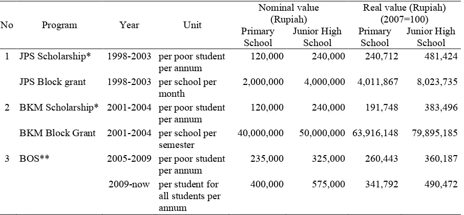
Table 2 shows a summary of the amount of assistance for each school subsidy program in Indonesia for basic education after the primary school construction project in the 1970s (SD Inpres program), from 1998 until now. There are three big programs which support basic edu-cation system in Indonesia. All of them have the goal of increasing net enrolment in primary and junior high school.
PROFILE OF STUDENTS AND BOS AT BASIC EDUCATION IN INDONESIA
The 9 year basic education goes from primary school to junior high school and these levels of schooling are a compulsory part of the structure of education in Indonesia. There are 6 main levels of schooling, from play group to university. First, play group is normally for children aged between 3-4 years. Second, kindergarten is usually for children aged between 5-6 years. Neither of these first two schooling after 9-year basic education and is not compulsory. Lastly, higher education is from undergraduate to post graduate programs.
The main goal of the 9-year basic education program and the BOS program is, therefore, to ensure that all Indonesian citizens attain the junior high school level free of charge. Currently, the net enrolment rate of junior high school in Indonesia is approximately 70 percent. By implementing the BOS program, the Goverment of Indonesia has set a target to achieve approximately 100 percent of junior high school gross enrolment rate or approxi-students at non-formal education equal to primary school level (could be elderly who enrol in non-formal education equal to primary school level) divided by the total number of people in that age of schooling and multiplied by 100 percent.
Net enrolment rate is calculated from the total number of students at primary school age (only those who enrol in formal education at primary school) divided by the total number of people in that age of schooling and multiplied by 100 percent. Gross enrolment rate could be more than 100 percent because there are students who are outside the official school age, for instance 25-year-olds who went to primary school. The same way is used to calculate the junior high school gross and net enrolment rates.
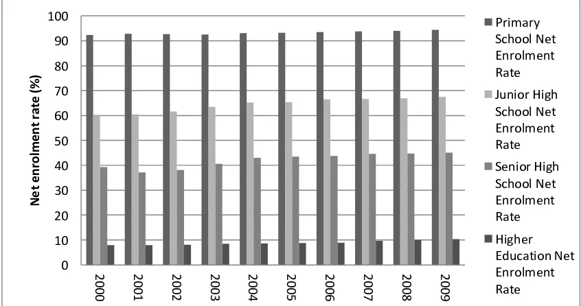
Figure 1 represents the net enrolment rate in each level of education from 2000 to 2009.
The figure shows that the highest net enrolment rate in Indonesia in 2009 is primary school at around 95 percent, followed by junior high school at approximately 70 percent. The net enrolment rate of senior high school is around 45 percent and the lowest one is university primary school and higher education net enrol-ment rate.
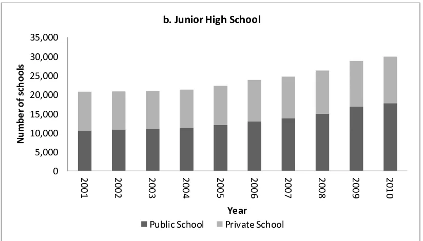
To achieve the net enrolment target, the Government of Indonesia has increased the number of junior high schools significantly. Figure 2 demonstrates the number of schools at primary school and junior high school levels from 2001 to 2010. There has been a significant rise in the number of junior high schools, both public and private, and a slight decrease in the number of primary schools in Indonesia from 2000 to 2010.
classrooms and classes in existing primary However, the trend in the number of junior high school students has shown a significant increase since 2005, especially for public schools (figure 3). This reflects the government’s commitment to provide a 9-year basic education.
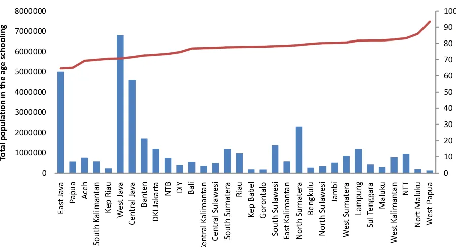
Based on the previous evidence, the govern-ment of Indonesia has made a significant effort to improve resources and to increase the net enrolment rate at every level of education. By implementing the BOS program, the government signalled its intention to increase the net enrolment rate, particularly for basic education. As can be seen in Figure 4, according to the regions in Indonesia is below 90 percent, except in West Papua. This is because West Papua has less children of school age than other provinces. In addition, regions with higher numbers of children of school age seem to have a lower enrolment, such as East Java, West Java and Central Java. In fact, there are still many children at the primary school level who do not receive BOS as their financial support to provide free access to basic education. These children are not registered at primary school level. It could be because they are categorised as street children, helping their parents to earn money, or their parents are not keen to encourage their children to go to school because they live in remote areas.
DATA SOURCES
The main source of the micro data used in this research is the Indonesia Family Life Survey (IFLS). In particular, this paper uses data from IFLS4 (2007). This study also uses school subsidies data from the Ministry of Education
and Culture of the Republic of Indonesia (MOEC) and other data from the Central Bureau of Statistics of Indonesia (BPS) such as: Net Enrolment Rate on Each Level of Schooling; Number of Schools for Primary and Junior High School Levels; and Number of Primary and Junior High School Students. IFLS provides educational information at individual, household and community levels. MOEC provides infor-mation about school subsidies at the aggregate level, and some demographic information comes from BPS.
1. BOS Data
This study only estimates the early version of BOS since it was launched in 2005 to enable poor students to have free access to basic education and this study uses IFLS survey data from 2007. This study determined BOS students based on self-reported information and generated BOS as a dummy variable equal to 1 if students reported that they received BOS and 0 other-15 percent at junior high school.
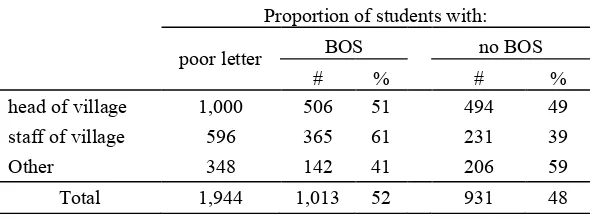
The number of students who receive BOS is lower than the government’s expectation and the data suggest that BOS is failing to support all students for all nine years of basic education. In comparison, a study by SMERU in selected regions in 2006 found that there were only a few poor students who received BOS from the total number of poor students in the study regions. Table 4 shows the number of poor students who received BOS from the school samples.
2. Student Test Score
Test scores are obtained from the tests in primary school at age 11 or in children’s final year of primary school. All questions in the test are multiple choice and are marked using of the test are announced a month later.
The test score is continuous variable and ranges from 0 to 10. It is calculated from the average scores of 3 subjects (Maths, Science and Indonesian Language). Test score data from the IFLS surveys are taken only from the respon-dents who could show test certificates and excludes the respondents who could not show certificates, since sometimes the information is not complete. For instance, they only mentioned 2 subjects out of 3 or they only mentioned the total score without mentioning each of the subjects individually, because they did not remember their scores in detail. Figure 9 presents the child test score distributions for BOS and non-BOS students.
Table 6 shows the descriptive statistics of test scores from BOS students and non-BOS students. BOS students have higher average test scores than non BOS students.
In addition, this study also performed t-test to test whether there were significantly different test scores between BOS and Non-BOS students. A t-statistic of -3.76 and a p-value 0.0002, half of students’ test scores below 6.5 out of 10 are from students whose parental backgrounds are not higher than junior high school. The highest test scores are found for students whose father’s education is at doctoral level.
3. Education Expenditure
Apart from school fees (such as registration fees, tuition fees and exam fees), there are also other education costs incurred during schooling, for instance: textbooks cost, uniform cost, transportation cost, housing and food cost, and any additional courses which students take outside school. Table 8 describes the various These registration fees are only paid once during their schooling in primary school and are set by the school committee (school teachers, school principal and student’s parent representative), and under the control of local government. The which are excluded from the school fees and are very significant expenses for each student are transportation costs, housing costs and food for students who live far away from their schools. These students need to rent a boarding house and spend some money for their own food. The housing costs and food costs are usually incurred for students at junior high school. If it compares the total school expenses to the amount of school subsidy which was shown in Table 2, the school subsidy is only sufficient for school fees or even only enough for tuition fees if the students live in urban areas. The remainder of the education expenditures must be covered by the household. That is why there are still some children of school age who cannot afford even basic schooling.
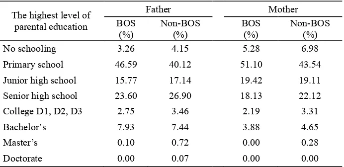
4. Parental Education Background
However, the proportion of parents with only primary education is higher for BOS students than non-BOS students. The higher the edu-cation level, the smaller the proportion of fathers and mothers. In general, however, the parents of non-BOS students are slightly more educated than BOS students.
RESEARCH METHODOLOGY: PROPENSITY SCORE MATCHING ESTIMATION
This study used matching method to get the estimation result from the average treatment effect in the absence of selection based on unobserved characteristics. Although random-ized evaluation is still a perfect impact evalua-tion method, sometimes a treatment cannot be randomized, so the best try is used a mimic randomization. It is an observational analogue of a randomized experiment. Matching methods try to develop a counterfactual or control group that is similar to the treatment group given of observed characteristics.
According to Blundell et al. (2005), the matching method is defined as a non-parametric approach that attempts to find a comparison group from all the non-treated so that the selected group is similar to the treatment group in term of their observable characteristics. The only remaining difference between two groups is participation in BOS program, therefore, the outcomes from the comparison group is the right sample for the missing information on the outcomes of the treatment group. Propensity Score Matching (PSM) estimation method is adopted when there is a wide range of matching variables. The World Bank argues that PSM is a useful approach when we believe that an observed characteristics affect program partici-pation and is sufficiently strong to determine program participation.
According to Rosenbaum & Rubin (1983), propensity score is a feasible method to match the variables by using balancing score. Blundell, Dearden & Sianesi (2005) said that, by defi-nition, propensity score matching is when treatment and non-treatment observations with the same value of propensity score have the
same distribution of density scores. Hence, PSM match treated and untreated observations on the estimated probability of being treated (propen-sity score).
This paper uses PSM to estimate the average treatment effect in the absence of selection on unobserved characteristics. PSM requires selection on observables assumption when conditioned on an appropriate set of observable attributes. Obviously, there is variability in selections that influences the selection process for the treatment group and the control group. should show a letter from the village head to the school committee. For those who can prove themselves as poor, they will receive a treat-ment.
In non-experimental studies, the essential problem is the missing counterfactual. PSM uses information from other students that do not get BOS (Non-BOS students) as a control group to identify what would have happened to students in the absence of the intervention (BOS). By comparing the outcomes from BOS students relative to observationally similar groups (non-BOS students), it is possible to estimate the effects of the intervention.
The PSM Model
treatment outcome or when �" is equal to one.
�*" is the potential outcome of individual i when
the individual does not receive BOS as control outcome, or when �" is equal to zero. Thus, the treatment effect for an individual can be written as the following equation:
�" = �&" − �*" (2)
The fundamental problem of causal infe-rence/counterfactual problem makes it impossi-ble to observe the potential outcome of indivi-duals for both treatment (�&" ) and control (�*") conditions at the same time, so only one poten-tial outcome for each individual can be observed, thus estimating the treatment effect of an individual is impossible.
This paper estimates the average treatment effect on the treated (ATET). ATET estimates the average among those who got the treatment or received BOS. ATET can be formulated as:
����� = �[�&"− �*"|�" = 1] (3)
����� = � � �" = 1
= � �&" �"= 1 − � �*" �" = 1 (4)
� �&" �" = 1 is the potential outcome of
students who receive BOS (BOS students) and is potentially observable. �[�*"|�" = 1] is the potential outcome of BOS students when they did not receive BOS and cannot be observed because it is the missing counterfactual.
To calculate ATET, it is essential to find a same time when those individuals received treatment. So, ATET can be estimated by using:
� �&" �" = 1 − � �*" �"= 0 = �����
...(5)
Hence, ATET is estimated from the potential outcome of BOS students who receive treatment,
� �&" �" = 1 , minus the potential outcome of
non-BOS students who did not receive treat-ment, � �*" �" = 0 .
Assumptions and Five Steps of PSM
In matching methods, there are assumptions to be applied in order to get a comparison group similar to the treatment group in observable characteristics (Sianesi, 2006):
1. Conditional Independence Assumption (CIA)
The potential outcomes are independent of the treatment assignment based on the obser-vable attributes of covariates X which are not influenced by treatment (Caliendo and Kopeinig, 2005). Here, the observable differences in characteristics between the treated group or BOS students and non-treated group or non-BOS students should be controlled; the outcome that would result in the absence of treatment is the same in both cases. This identifying assumption for matching, which is also the identifying assumption for the simple regression estimator, is known as the Conditional Independence Assumption (CIA).
2. Common Support
Common support is the condition when there is a region of the support of matching variable that overlaps with the distribution of density scores from treated and untreated groups. The treated and untreated individual must have similar probabilities or treatment. As illustrated by figure 10, the region of common support is the range of the score which overlaps between density of scores for untreated individuals and density of scores for treated individuals.
The data can be estimated by using the five steps of Propensity Score Matching (PSM) Estimation. The five steps are as follows:
1. Estimate the Propensity Score
Moreover, for the choice of variables, the choice must be based principally on economic theory and previous empirical research findings.
2. Choosing a Matching Algorithm
There are a few different matching algo-rithms. According to Caliendo and Kopeinig (2006), the matching algorithms are divided into five different groups: Nearest Neighbour(NN), Caliper and Radius, Stratification and Interval, Kernel and Local Linear and Weighting (see better matches because controls that look similar to many treated units can be used multiple times, and the order in which the treated units are matched does not matter. In the case of NN without replacement, the ordering has to be done before estimating.
3. Having Common Support
Common support is a critical step in matching estimation. This depends on whether or not overlap occurs between treated and non-treated groups. The common support condition ensures that matches for treated and untreated groups can be found.
4. Assessing the Match Quality
Tests must be conducted to assess the matching quality, such as test for standardised bias, test for equality of means before and after matching (t-test) and test of joint equality of means in the matched sample (F-test). If there is bad matching quality or there are still any differences, it is better to take a step back and redo the same steps until the matching quality is satisfactory. If after specification and re-assessment the matching quality and the results are not satisfactory, it indicates that the Condi-tional Independence Assumption fails to be met
and alternative evaluation approaches should be used.
5. Estimating the Standard Errors and Sensitivity Analysis.
To deal with the problem of understated standard errors because of variation beyond the normal sampling variation when estimating, Lechner (2002) suggests using bootstrapped standard errors. Bootstrapped standard errors are used when the sampling distribution of para-meter may not be of any standard distribution. Bootstrapped standard errors rely upon the assumption that the current sample is represen-tative of the population. Besides that, sensitivity analysis should be applied to estimate the level of bias in observational studies (Guo and Fraser, 2010). Based on Rosenbaum and Rubin (1983) and Rosenbaum (2005), sensitivity analysis should be conducted routinely to see sensitivity of findings to hidden bias when the treated and untreated groups may differ in ways that have not been measured. Wilcoxon’s signed-rank test is one method of sensitivity analysis that was developed by Rosenbaum (2002).
EMPIRICAL RESULTS
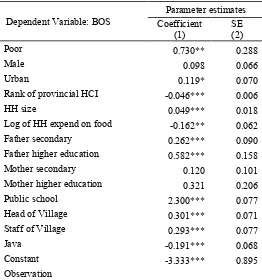
deter-mined by various individual characteristics, e.g., gender, poor dummies, rank of province based on head count index, household expenditure on food, area, school administration and parental education background. Table 10 shows the results of the logit model.
Looking at Column 1 of Table 10, most variables are significant at typical significance levels and only a few variables are not. The variables poor, urban, public school, rank of provincial HCI, the number of household members (hhsize) and household expenditures on food are significant. Those variables have the most influence on the probability of getting a school subsidy.
1. Choosing Matching Algorithms
This study uses Near Neighbour Matching, since the distribution of data is a little different in treated and untreated groups. As shown in Figure 12, the distribution of the treated group seems to have a higher propensity score than the untreated group which is what is supposed to happen.
2. Checking the common support
Following Sianesi (2006), the common support should be checked. The common support condition requires that there exists treated and non-treated units with similar values of the propensity score after matching. Figure 13 confirms that the common support holds. There is an overlap propensity score between treated and control groups.
3. Assessing the match quality
In order to check the success of the matching for all independent variables, there are some tests to be done after matching. Caliendo and Kopeinig (2005) suggest assessing the quality of matching by using a standardised bias test, t-test for testing the equality of means before and after matching and an F-test for the joint equality of means in the matched sample.
3.1. Test of standardised bias
The standardised bias test is used to check the reduction of bias after matching. According
to Rosenbaum and Rubin (1985), the stan-dardised bias approach is calculated from the difference in means of the treated and untreated variables as a percentage of the square root of the average variance in both groups.
Table 11 shows the standardised bias of variables before and after NN matching. We see 8 out of 14 of the variables have less bias after matching than before matching, although 6 variables have a higher bias after matching. Caliendo and Kopeinig (2005) stated that there is no clear standard of success for bias reduction in matching methods.
3.2. Test for equality of the mean before and after matching (t-test)
Rosenbaum and Rubin (1985) also suggested a t-test of the difference of covariate means for treated and control groups. Table 12 displays the p-value of the t-test for equality of the means before and after matching. Before matching, some of the covariate means are different between treated and control groups, but after matching only one (child test score) is signifi-cantly different between groups.
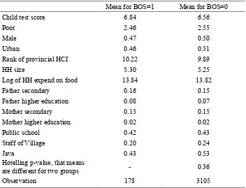
3.3. Test of Joint Equality of Means in the Matched Sample (Hotelling Test)
After testing the difference of covariate means individually, a joint test for equality of means in all covariates can be conducted. Using the Hotelling test in Stata, the result shows that the P value of the F test is greater than 5 percent, which is 0.36. It indicates that the null of joint equality of means is not rejected, so the conditioning variables are well balanced jointly.
RESULTS
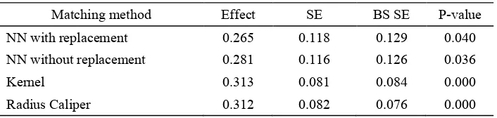
replace-ment. For individuals in the treatment group, the treatment has raised the test score by 0.26 points on average for NN matching with replacement, and by 0.28 points on average for NN without replacement. To check that the results are robust, this study carried out a number of additional estimation experiments with different matching estimators. In particular, it has tested calliper matching and also kernel matching. Table 14 shows the various results from several types of matching methods and the estimated treatment effects are very similar to those obtained from NN with replacement and without replacement.
EVALUATION: SENSITIVITY ANALYSIS
According to Rosenbaum (2002), selection bias occurs when two individuals with the same observed covariates have a different probability of receiving treatment. To deal with selection or hidden bias, Rosenbaum suggested that sensi-tivity analysis be conducted using Wilcoxon’s signed rank test to get Rosenbaum bounds. Table 15 shows the results of this sensitivity analysis for the study of the effect of the school subsidy on students’ tests scores using Wilcoxon’s signed rank test. The point estimation of Rosenbaum’s bounds of this study for the p-values with Γ=1 is very close to the estimation in the propensity score matching analysis. The estimation effect of NN matching is 0.26 and the Hodges-Lehman point estimate is 0.269 and both results are significant at 5 percent.
Table 15 also shows that for a small increase of Γ=0.2, p value increases to 0.099 in the upper bound, which is above the threshold of p value 0.05. In this case, a hidden bias or selection bias of size Γ=1.2 is sufficient to explain the observed difference in test scores between the treatment group and the control group. Hence two units that appear similar and have the same covariates could differ in their odds of receiving the treatment by as much as a factor of 1.2. Because 1.2 is a small value, it shows that this study is sensitive to hidden bias. For Hodges-Lehman point estimate interpretation, for example when Γ=1.1, matched students might differ in their test scores by a factor of 1.1 due to
hidden bias. The range is between 0.206 and 0.332.
CONCLUSIONS
This research indicates that poorer students have lower average test scores. This finding suggests that the Government of Indonesia needs to develop a subsidy program to provide a basic level of education for all students, especially for the poor. The recent school subsidy program is only sufficient for school fees or even only enough for tuition fees if the students live in urban areas. The remainder of the education expenditures must be covered by the household. That is why there are still some children of school age who cannot afford even basic schooling. This finding suggests that the amount of school subsidy should be adjusted and recalculated based on total education expen-diture including transportation costs, living costs, book costs, and uniform costs.
Another important finding is that parental education background is positively related to test scores. Moreover, estimation using PSM suggested that the BOS program has a positive and significant effect on child test scores. Students who receive subsidies attain higher test scores. It suggested that the BOS program in Indonesia increased test scores by 0.26 points or 21.3percent of standard deviation. Overall, the early version of the program, BOS successfully improved student test scores performance. As a school subsidy policy, BOS is good at helping poor students to get access to education, especially basic education, since the government can ensure the use of subsidy for schooling, as Development Economics, 92, 152-165. Angrist, J. D., & Krueger, A., 1991. Does
Angrist, J. D., & Pischke, J.-S., 2009. Mostly Harmless Econometrics An Empiricist's Companion. Princeton USA: Princeton University Press. theoritical Analysis with Special Reference to Education. New York: The National Bureau of Economic Research.
Behrman, J. R., & Todd, P., 1999. Randomness in the experimental samples of PREGRESA (Education, Health, and Nutrition Program). International Food Policy Research Institute.
Blundell, R., Dearden, L., & Sianesi, B., 2005. Evaluating the effect of education on earnings: Models, methods and results from the national child development survey. Royal Statistics Society, 168(3), 473-513. Caliendo, M., & Kopeinig, S., 2005. Some
Practical Guidence for the Implementation of Propensity Score Matching. IZA Institute for the Study of Labor, Discussion paper no.1588.
Card, D., 2001. Estimating the Return to Schooling:Progress on Some Persistent Econometric Problem. Econometrica, 69(5), 1127-1160.
Dearden, L., & Heath, A., 1996. Income Support and Staying in School: What Can We Learn from Australia's AUSTUDY Experiment? Institute for Fiscal Studies, Vol.17, No.4, 1-30.
Dearden, L., Emmerson, C., Frayne, C., & Meghir, C., 2005. Education Subsidies and School Drop-Out Rates. The Istitute for Fiscal Studies, Working paper no.WP05/11. Dehejia, R. H., & Wahba, S., December 1998.
Propensity Score Matching Methods For Non-Experimental Causal Studies. National Bureau of Economic Research, NBER Working Paper No.6829.
Duflo, E., 2001. Schooling and Labor Market Consequences of School Construction in Indonesia: Evidence from an Unusual Policy Experiment. The American Economic Review, 91(4), 795-813.
Glewwe, P., & Olinto, P., 2004. Evaluating the Impact of Conditional Cash Transfers on Schooling: An Experimental Analysis of Honduras' PRAF Program. Final Report of USAID.
Guo, S., & Fraser, M., 2010. Propensity Score Analysis Statistical Methods and Appli-cations. London: SAGE Publication Ltd. Imbens, G. W., & Angrist, J., 1994.
Identi-fication and Estimation of Local Average Treatment Effects. Econometrica, 62(2), 467-475.
Janvry, A. d., & Sadoulet, E., 2006. Making Conditional Cash Transfer Programs More Efficient: Designing for Maximum Effect of the Conditionality. World Bank Economic Review, 20(1), 1-29.
Kim, J., Alderman, H., & razem, P., 1999. Can Private School Subsidies Increase Enrollment for the Poor? The Quetta Urban Fellowship Program. The World Bank Economic Review, 13(3), 443-465.
Lechner, M., 2002. Some practical issues in the evaluation of heterogenous labour market programmes by matching methods. Journal of the Royal Statistical Society, A(165), 59-82.
Maluccio, J. A., & Flores, R., 2005. Impact Evaluation of Conditional Cash Transfer. International Food Policy Institute, Research report no.141, 1-66.
Riccio, James, Dechaussay, N., Greenberg, D., Miller, C., Rucks, Z., & Verma, N., 2010. Toward Reduced Poverty Across Gene-rations: Early Findings from New York City’s Conditional Cash Transfer Program. New York: MDRC.
Rosenbaum, P. R., 2005. Sensitivity analysis in observational studies. Encyslopedia of statistics in behavioral science, 4, 1809-1814.
Rosenbaum, P. R., & Rubin, D., 1983. The Central Role of the Propensity Score in Observational Studies for Causal Effects. Biometrica, 70, 41-45.
Schady, N., & Araujo, M., 2008. Cash Transfer, Conditions, and School Enrollment in Ecuador. ECONOMIA.
poverty program. Journal of Development Economic, 74, 199-250.
Sianesi, B., 2001. Implementing Propensity Score Matching Estimators with Stata. UK Stata Users Group, VII Meeting. London: University of College London and Institute for Fiscal Studies.
Sparrow, R., 2007. Protecting Education for the Poor in Times of Crises: An Evaluation of a
Scholarship Programme in Indonesia. Oxford Bulletin of Economics and Statistics, 69 (1), 99-122.
Table 1. The Effect of School Subsidies in Various Countries
Study Country Marginal effect Prop of SD Dependent variable
Dearden and Heath (1999) Australia 0.038 7.70% enrolment rate
Dearden et al. (2005) UK 0.045 7.20% dropout rate
Schultz (2004) Mexico
Female 0.0092 4% enrolment rate
Male 0.008 3% enrolment rate
Schady and Araujo (2004) Ecuador 0.032 7.60% enrolment rate
Afridi (2010) India
Girls 1st grade 1.768 5.50% enrolment rate Kim, Alderman and Orazem (1999) Pakistan 0.33 68% enrolment rate
Glewwe and Olinto (2004) Honduras 0.02 2.20% enrolment rate
Maluccio and Flores (2005) Nicaragua 0.128 19.39% enrolment rate
Sparrow (2007) Indonesia 0.008 2.60% enrolment rate
Duflo (2001) Indonesia 0.03 17.60% dropout rate
This study (2012) Indonesia 0.26 21.3% test score
Note: SD=Standard Deviation
Table 2. The Amount of School Subsidies
No Program Year Unit
Nominal value (Rupiah)
Real value (Rupiah) (2007=100) Primary
School
Junior High School
Primary School
Junior High School 1 JPS Scholarship* 1998-2003 per poor student
per annum
120,000 240,000 240,712 481,424
JPS Block grant 1998-2003 per school per month
2,000,000 4,000,000 4,011,867 8,023,735
2 BKM Scholarship* 2001-2004 per poor student per annum
120,000 240,000 191,748 383,496
BKM Block Grant 2001-2004 per school per semester
40,000,000 50,000,000 63,916,148 79,895,185
3 BOS** 2005-2009 per poor student per annum
235,000 325,000 260,443 360,187
2009-now per student for all students per annum
400,000 575,000 341,792 490,472
Table 3. BOS Participation Rate
Primary School Grade Percentage of student Number of students
Non BOS BOS
1 85.51 14.49 856
2 81.89 18.11 795
3 84.07 15.93 703
4 83.46 16.54 665
5 85.03 14.97 715
6 87.02 12.98 131
Junior High School Grade
1 87.35 12.65 490
2 85.25 14.75 400
3 85.02 14.98 227
Source: calculated from IFLS 4
Table 4. The Percentage of Poor BOS Students in Selected Samples
Province Total number of Students
Poor students Poor students with BOS
Number % of total
students Number
% of total students
% of total poor students
East Java 2957 1002 33.9 242 8.2 24.2
North Sulawesi 3173 - - 296 9.3 -
North Sumatra 2841 940 33.1 256 9 33.1
West Nusa Tenggara 1740 568 32.6 111 6.4 32.6
Source: SMERU 2006
Table 5. Proportion of Students by Village Decision Maker
Proportion of students with:
poor letter BOS no BOS
# % # %
head of village 1,000 506 51 494 49
staff of village 596 365 61 231 39
Other 348 142 41 206 59
Total 1,944 1,013 52 931 48
Source: calculated from IFLS data
Table 6. Students’ Test Score in 2007
BOS Non-BOS
Mean 6.56 6.50
SD 1.36 1.25
Observation 276 6320
Table 7. Distribution of Students’ Test Score by Parental Education Background (%)
The highest level of parental education
Father education Mother education
Average test score % Average test score %
No schooling 6.26 4.76 6.24 7.97
Primary school 6.40 48.93 6.40 54.78
Junior high school 6.46 15.47 6.53 16.24
Senior high school 6.66 22.12 6.85 16.05
College D1, D2, D3 6.96 2.90 7.02 2.63
Bachelor’s 7.03 5.45 7.06 2.22
Master’s 7.26 0.33 7.70 0.11
Doctorate 8.35 0.03
Observation 6405 6528
Source: calculated from IFLS data
Table 8. The Average Costs to Individuals of School Spending (Rupiah) per annum in 2007
Variable Rural Urban
Registration fees 58,250 234,369
Tuition fees 83,800 317,748
Exam fees 16,833 40,262
Book costs 66,687 134,050
Uniform costs 62,942 112,433
Transportation costs (A) 134,215 282,019 Housing costs and food (B) 299,338 560,758 Additional course costs (C) 20,803 96,588
Total 742,868 1,778,227
Total – (A+B+C) 288,512 838,862
Source: calculated from IFLS4; Note: 1 USD= 14,000 Rp
Table 9. Parental Education
The highest level of parental education
Father Mother
BOS (%)
Non-BOS (%)
BOS (%)
Non-BOS (%)
No schooling 3.26 4.15 5.28 6.98
Primary school 46.59 40.12 51.10 43.54
Junior high school 15.77 17.14 19.42 19.11
Senior high school 23.60 26.90 18.13 22.12
College D1, D2, D3 2.75 3.46 2.19 3.31
Bachelor’s 7.93 7.44 3.88 4.65
Master’s 0.10 0.72 0.00 0.28
Doctorate 0.00 0.07 0.00 0.00
Table 10. BOS Logit Model
Dependent Variable: BOS
Parameter estimates Coefficient
(1)
SE (2)
Poor 0.730** 0.288
Male 0.098 0.066
Urban 0.119* 0.070
Rank of provincial HCI -0.046*** 0.006
HH size 0.049*** 0.018
Log of HH expend on food -0.162** 0.062
Father secondary 0.262*** 0.090
Father higher education 0.582*** 0.158
Mother secondary 0.120 0.101
Mother higher education 0.321 0.206
Public school 2.300*** 0.077
Head of Village 0.301*** 0.071
Staff of Village 0.293*** 0.077
Java -0.191*** 0.068
Constant -3.333*** 0.895
Observation
Note: dependent variable is BOS where 1 is for recipient and 0 otherwise *Significant at 10%, **significant at 5%, ***significant at 1%
Table 11. Standardised Bias from NN Matching
Before
Matching
After Matching
Child test score 30.1 24.7
Poor 4.6 -6.5
Male -9.3 -7.9
Urban -12.2 -9.0
Rank of provincial HCI -4.5 5.6
HH size 8.3 5.1
Log of HH expend on food -5.0 0.7
Father secondary -14.3 2.9
Father higher education 16.7 4.5
Mother secondary -0.2 -1.6
Mother higher education 0.5 -7.7
Public school -7.8 -1.1
Staff of Village 1.2 -8.5
Table 12. Test for Equality of The Mean Before and After Matching (t test)
P value of t test
Before matching NN with replacement
Child test score 0.000 0.024
Poor 0.566 0.548
Male 0.228 0.459
Urban 0.112 0.397
Rank of provincial HCI 0.540 0.598
HH size 0.320 0.615
Log of HH expend on food 0.522 0.947
Father secondary 0.076 0.772
Father higher education 0.012 0.695
Mother secondary 0.978 0.884
Mother higher education 0.948 0.476
Public school 0.309 0.915
Staff of Village 0.880 0.439
Java 0.019 0.056
Table 13. Hotelling Test After Matching
Mean for BOS=1 Mean for BOS=0
Child test score 6.84 6.56
Poor 2.46 2.55
Male 0.47 0.50
Urban 0.46 0.51
Rank of provincial HCI 10.22 9.89
HH size 5.30 5.25
Log of HH expend on food 13.84 13.82
Father secondary 0.16 0.15
Father higher education 0.08 0.07
Mother secondary 0.15 0.15
Mother higher education 0.02 0.02
Public school 0.42 0.43
Staff of Village 0.20 0.24
Java 0.43 0.53
Hotelling p-value, that means
are different for two groups - 0.36
Table 14. The Effect of School Subsidy on Student Performance
Matching method Effect SE BS SE P-value
NN with replacement 0.265 0.118 0.129 0.040
NN without replacement 0.281 0.116 0.126 0.036
Kernel 0.313 0.081 0.084 0.000
Radius Caliper 0.312 0.082 0.076 0.000
Note: SE(Standard Error of estimator); BS SE(Bootstraped clustered standard error)
Table 15. The Rosenbaum Sensitivity Analysis
Γ p-value of Wilcoxon’s signed-rank test Hodges-Lehman point estimate Upper bound Lower bound Upper bound Lower bound
1 0.010 0.010 0.269 0.269
1.1 0.037 0.002 0.206 0.332
1.2 0.099 0.000 0.153 0.391
1.3 0.203 0.000 0.102 0.439
1.4 0.341 0.000 0.050 0.492
Source of data: Central Bureau of Statistics Indonesia (Badan Pusat Statistics, BPS)
Source of data: Central Bureau Statistics of Indonesia (Badan Pusat Statistics, BPS)
Figure 2. The Number of Schools for Primary and Junior High School Levels 0
2001 2002 2003 2004 2005 2006 2007 2008 2009 2010
Source of data: Central Bureau Statistics of Indonesia (Badan Pusat Statistics, BPS)
Figure 3. The Number of Primary and Junior High School Students
Source: Ministry of Education and Culture of the Republic of Indonesia
Figure 4. Ratio of BOS Students to Total Number of Children at Primary School Age in 2010 by Region
2001 2002 2003 2004 2005 2006 2007 2008 2009 2010
Figure 5. Proportion of Students with BOS by Village Decision Maker
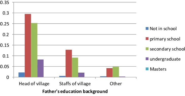
Figure 6. Proportion of Father’s Education Background from BOS Students by Village Decision Maker
0.00 0.01 0.02 0.03 0.04 0.05 0.06
head of village staffs of village other
P
ro
p
o
rt
io
n
o
f
B
O
S
s
tu
d
e
n
ts
0 0.05 0.1 0.15 0.2 0.25 0.3 0.35
Head of village Staffs of village Other
Father's education background
Not in school
primary school
secondary school
undergraduate
Figure 7. Proportion of Gender from BOS Students by Village Decision Maker
Figure 8. Proportion of Urban/Rural from BOS Students by Village Decision Maker
Figure 9. Test Scores Distribution 0
0.05 0.1 0.15 0.2 0.25 0.3 0.35 0.4
Head of village Staffs of village Other
Proportion of BOS students by gender
female
Figure 10. Common Support Region
Source: Caliendo and Kopeining (2006)
Figure 11. Different Matching Methods Matching
Algorithms
Weighting
Kernel and Local Linear Stratification and Interval Caliper and Radius Nearest Neighbour (NN)
With/without replacement,
oversampling, weights for oversampling
With tolerance level (caliper), 1-NN only or more (radius)
Number of strata/interval
Kernel functions, bandwidth parameter
Figure 12. The comparison of propensity score distribution before matching