Constraints in vision
Outline of a set-theoretic approach
* Luigi Burigana `
Universita degli Studi di Padova, Dipartimento di Psicologia Generale, Via Venezia, 8, I-35131 Padova, Italy
Accepted 1 November 1998
Abstract
The idea is advanced that the highly complex relationship between stimuli and percepts in vision may be formally described as an extensive system of relational constraints, involving both stimulus and perceptual variables; some guidelines are also suggested for working out this idea and applying it to salient general questions of vision research. The paper starts by defining the basic notions of located variable and located constraint (Sections 2 and 3) with respect to a presumed homogeneous set of observational situations. Then the most important notions of a system of constraints and of pairing between a system of constraints and an assignment of values to stimulus variables are introduced (Sections 4 and 5). A set-theoretic way of representing the combined predictive power of such pairing is suggested, and some elementary properties of the concept are described. Lastly, a few comments are made on the possible use of the constraint paradigm in discussing some critical aspects of contemporary research on vision and some reasons are given for the suggested set-theoretic approach (Sections 6 and 7). 1999 Elsevier Science B.V. All rights reserved.
1. Introduction: the multiple constraint paradigm
An observer has a visual experience when he / she looks at some portion of the surrounding physical reality. In a very general sense, the task of the science of vision is to study how the data in visual experience depends on optically important aspects of the observed reality or, more properly, how the contents in the resulting phenomenal scene depend on the given stimulus conditions. There are different ways of conceiving and pursuing such a general task. For example, one may study vision by trying to discover or
*Tel.: 139-49-827-6668; fax:139-49-827-6600. E-mail address: [email protected] (L. Burigana)
reconstruct ‘‘perceptual processes’’, i.e., examining the complex dynamics (transforma-tions, causa(transforma-tions, integra(transforma-tions, etc.) which presumably take place in the visual system, starting from the entering stimuli and ending with the perceptual response. Alternatively, vision may be studied by recording, analysing and combining regular relations between stimulus and perceptual data, as they are directly established through experimentation, without entering into the features of the underlying processes. We may qualify such alternative perspectives as the ‘‘genetic’’ and the ‘‘descriptive’’ approaches to the study of vision, thus applying a distinction used long ago by Franz Brentano for psychology in general (cf. Mulligan and Smith, 1988). The former is qualified as a genetic approach because it is directed to the reconstruction of the ‘‘genesis’’ or formation processes of perceptual results; the latter is qualified as a descriptive approach because all terms it refers to are observable (through direct perception or by optico-physical measurement) and it aims at an ordered and parsimonious representation of the network of relations connecting such terms.
The ideas we have in mind to expound in this paper are specifically related to the latter perspective, i.e., the descriptive approach in perceptual science. Questions concerning processes in the visual system are virtually extraneous to our analysis (except for one isolated mention in the last but one section). Even so, the set of concepts we find necessary in applying the descriptive approach proves to be quite complex, as different requirements and rules of variation come into play. (i) First of all, a distinction must be drawn between some levels of data, each level being qualified by a certain position in the organization of an observational case (perceptual episode) and by a certain way of empirical assessment. Specifically, we will refer to an S-level (the level of external surfaces, or distant stimuli), which is the set of optically relevant properties of the observed reality, as they may be measured through optico-physical procedures; an I-level (the level of retinal images, or proximal stimuli), which is the set of effects or conditions on the eye, as they may be determined by means of optical measurement or computation; and a P-level (the level of perceptual data), the set of contents in the perceptual scene, as it is directly experienced by the observer. (ii) At each level, distinction must be made between several types of data: at the P-level, for example, one may distinguish between colours, lightnesses, lengths, distances, orientations, etc., which represent separate kinds of possible contents in perceptual scenes. Under certain conditions, in relation to a presumed multiplicity of observational cases, each type of data defines a type of variable (a non-located variable) which may be referred to such multiplicity. Distinction may be made between S-, I- and P-variables, depending on whether the values they take on are data belonging to the S-, I- or P-levels. (iii) Further, we must consider a variety of
constraints, which are here conceived as dependence relations acting on definite groups
represents a large part of the power of stimulus conditions in specifying a selected perceptual aspect. As a rule, different perceptual problems lead us to consider different systems of constraints presumed to be relevant for them.
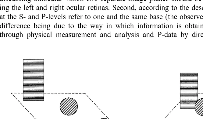
Let us illustrate these various concepts with the schematic example in Fig. 1, which refers to the problem of visual recovery of depth, i.e., the problem of perception of distances and relative positions in the third dimension. In the following picture, the observer’s position corresponds to the image plane, which represents the eye (more properly, the retina). Images projected on this plane by objects in the external world, as well as attributes and relations inherent in the images, are elements of the I-level of data. In this example, the observed portion of physical reality (the so-called layout of physical surfaces) consists of three planar objects lying perpendicular to the line of sight: a rectangle on the left, a disc in the centre, and another rectangle on the right. The three physical objects and all their optically relevant properties (physical shape, size, reflectance, distance from the observer and from one another, etc.) are part of the S-level of data. By looking at such a physical scene, the observer will experience a certain perceptual scene, supposedly comprised of three separate units, just like its physical counterpart. The three perceptual units and all their perceptual properties (apparent shape, size, lightness, phenomenal egocentric and exocentric distances, etc.) are elements of the P-level of data. Three simple comments are in order here. First, for the sake of simplicity, the observer is represented in Fig. 1 by a single image plane, but in discussing binocular vision two separate image planes should be considered, represent-ing the left and right ocular retinas. Second, accordrepresent-ing to the descriptive approach, data at the S- and P-levels refer to one and the same base (the observed piece of reality), the difference being due to the way in which information is obtained: S-data are gained through physical measurement and analysis and P-data by direct visual observation.
Third, again for simplicity, we presume here that there is an exact correspondence between units in the physical and the perceptual scene, but this is not a general rule at all: there are cases in which perceptual organization thoroughly modifies the articulation of the scene (see, for example, the case of phenomenal transparency, discussed in Section 3).
analysis shows that a certain relationship is at work between these variables (binocular disparity can be computed from distances), which represents a new example of SI-constraint. We may also consider the transposed relationship, which connects binocular disparity with the apparent distances of the rectangles, as they are seen by the observer: this is an example of IP-constraint. Similar constraints may also be specified in comparing either rectangle with the disc. Now, in addressing the problem of perceptual recovery of depth positions, a variety of such relational constraints must be considered, together with other kinds of constraints, which are related to other stimulus cues for distance (convergence, perspective, relative size, etc.). These various constraints, acting on specific subsets of an exhaustive set of variables, make up a system of located constraints.
The example just described is relatively simple when compared with observational situations in real life, and yet it suffices to illustrate the following notable circumstance: when the descriptive approach is applied to perceptual problems endowed with some articulation (say, not problems on isolated stimulus–percept correspondences, as are treated in elementary psychophysics), the components in the observational context that are presumably relevant for a given problem make up a heterogeneous set of relations, which may be represented as a system of constraints acting on a definite set of variables. Besides stimulus–percept or psychophysical relations (SP- and IP-constraints), the system may comprise percept–percept or intra-perceptual relations (P-contraints); besides binary relations (acting on selected pairs of variables), there may be constraints of a higher order (ternary, quaternary, etc.); further, some constraints in the system may be of different types, some others may be of the same type but differ from one another in location (i.e., the subsets of variables on which they act). In the following, we will call this way of representing and addressing perceptual problems the multiple constraint
paradigm (MCP). Our view is that this paradigm is the natural evolution of the
descriptive approach, when it is faced with perceptual problems of some structural complexity.
The proposed name is our own, but the essential features of MCP are distinctly seen in some significant branches of modern perceptual science. For example, the paradigm is implicit in studies on integration of visual modules, concerning how several elementary processes which are relevant for a certain perceptual aspect (e.g., various cues to distance, or various factors for solid shapes) may interact with each other, and combine their effects in an inequivocal and coherent result (cf. Aloimonos and Shulman, 1989;
¨
Bulthoff, 1991; Pankanti and Jain, 1995; Uttal et al., 1996). The paradigm is also at the basis of studies on multiple recovery in vision, such as the recovery of ‘‘surface shape and orientation from texture’’, ‘‘surface shape, albedo, and illuminant direction from shading’’ and ‘‘object shape and rotation sense from kinetic depth effect’’, in which distinct aspects of the perceptual scene are seen to derive from one set of stimulus data (Witkin, 1981; Todd and Mingolla, 1983; Ramachandran, 1988; Zheng and Chellappa, 1991; Nawrot and Blake, 1993).
Epilogue to their book on ‘‘integration of visual modules’’ state that ‘‘we need a formal theory for combining information from different sources’’ (Aloimonos and Shulman, 1989, p. 267). The aim of the present paper is to suggest some simple ideas on this issue, i.e., to draw a minimal conceptual frame for MCP, by defining and relating a few concepts which appear to be implicit in all its applications. Identifying and making explicit the basic concepts in a rigorous way is an initial and necessary stage for undertaking formal analysis of the paradigm, its conditions and implications.
The language we adopt for this formalization is elementary set theory, in order to ensure wide generality to the fundamental concepts, and to obtain a system that is flexible and faithfully applicable to various specifications of MCP (more detailed arguments for the set-theoretic approach will be presented in the concluding section). The main concepts are introduced progressively, starting from variables (Section 2), moving to constraints (Section 3), systems of constraints (Section 4), and pairings between systems of constraints and valuations of stimulus variables (Section 5). Besides definitions of these various concepts, some of their immediate facts and relationships will be noted, as the result of an initial inquiry into their formal properties. The paper makes use of some simple examples from perceptual science in order to illustrate the defined concepts, but it offers no fully extended demonstration of the adequacy of the suggested apparatus in dealing with specific research problems on vision. Nevertheless, in Section 6 we will mention and comment on some key concepts of current approaches to the study of vision which may be expressed, linked and clarified by using terms of the suggested conceptual system.
2. Variables and valuations
Intuitively, the concept of a variable refers to some kind of results that are (partially) different or unstable along a series of observations. Equally, the concept of a variable demands some stability along that series: results must be homogeneous to some extent, and must refer to a common and permanent base, so that they may be properly qualified as different values of one and the same variable.
These obvious requirements lead to the first components of our theoretical construc-tion. First, a set O of possible observational cases is presumed, each case o[O being a
closed perceptual episode, which comprises data at separate empirical levels (primarily, the S-, I- and P-levels defined in the Introduction). Second, we assume a well-defined set
U of recurrent units (i.e., specific objects or events, or selected parts of objects or
events); each unit u[U is presumed to occur (at a fixed level of data) in all cases in O,
with stable identity but with possibly and partly changing properties. Set U of recurrent units will serve as the required stable base for variable identification.
In relation to the given set O of observational cases, a located variable v is
determined by three aspects: type X , as a complete set of admissible values for thev
variable, state-function s , as a function from O to X , and location l , which is a subsetv v v
of set U of recurrent units. Type X is here conceived as an abstract and homogeneousv
corresponding value s (o) of function s is a point in X , which represents the valuev v v
taken on by variablevin case o. Location l is the carrier (as a system of recurrent units)
v
of the properties which constitute the values of variable v. Location l is a singleton
v
u #U, if X is a type of attributes or unary properties (e.g., a continuum of possible
h j v
reflectances), a pair u, uh 9j#U, if X is a type of binary properties or relations (e.g., av
complete set of admissible distances), and so on. We presume that the unit (or combination of units) acting as the location of a given variable, and the properties taken on as values by that variable, belong to a specific level of data, which remains the same along all cases in O, so that it makes sense to distinguish between S-variables (physical aspects or conditions of the observed realities), I-variables (properties in the proximal images of those realities) and P-variables (contents of the corresponding perceptual scenes).
Now, besides O and U, a third basic set for our theorization must be introduced. This is a collection V5hv , . . . ,v jof located variables, which are jointly defined in universe
1 m
O of observational cases. Set V is presumed to be exhaustive, in that it contains all
variables that are relevant for a fixed perceptual problem; each variablev (i51, . . . , m)
i
is qualified by some type X , a definite state-function s :Oi i →X , and a specific locationi
li#U. Set V must be imagined as a highly heterogeneous collection which assembles
attributive and relational variables, variables of different types, and variables of the same type but with different locations. In particular, set V may contain variables referring to distinct levels of data, i.e., S-, I- and P-variables. Put M5h1, 2, . . . , m , which is thej Y and X are used here for the set of all (partial) valuations and, respectively, for its
subset of complete valuations; moreover, for any K#M, symbol YuK denotes the set of
all valuations on coordinates in K (i.e., YuK5
h
y[Y: Muy5K , in particular Yj
uM5X ).These are the natural reference sets for the combinations of values taken on by sets of variables. In fact, for any o[O, the joint state of a set of variables W5
h
v , . . . ,vj
ini1 ik
the observational case o can be described as the set of pairs W(o)5h(i , s (o)), . . . , (i ,1 i 1 k
s (o)) , which is a point in Y (more specifically, in Yik j u(MuW )). Accordingly, set W(O )5hW(o): o[O of the joint states of W in all the observational cases amounts to aj subset of Y (more specifically, of Y(MuW )). In particular, for any case o, joint state V(o)5h(1, s (o)), . . . , (m, s (o)) of the entire set of variables V is a complete valuation,1 m j
and the exhaustive set V(O )5hV(o): o[O of such joint states is a subset of X.j Compatibility between valuations, denoted by symbol ↔, plays an important role in the following, and is defined as follows: any two valuations y, y9[Y are compatible
with each other if coincidence of some of their pairs in the coordinates implies coincidence of the same pairs in the values or, formally:
9 9 9 9
These facts are immediate: y#y9implies y↔y9(inclusion between valuations, as sets of pairs, ensures compatibility), if Muy#Muy9then y↔y9implies y#y9, if Muy>Muy9 5 5 (the two valuations are separate, i.e., they act on disjunct sets of coordinates) then
y↔y9. It is also directly seen that y↔y9 iff y<y9[Y, i.e., compatibility of two
valuations means that their union is itself a regular valuation.
Compatibility is first used in defining some basic operations on sets of valuations. Let
T,Z be subsets of Y. The restriction of T with respect to Z and the disjunction of the two
sets are specified by the following formulae:
r(T, Z )5ht[T : t↔z for some z[Zj
d(T, Z )5hy[Y: y5t<z for some t[T, z[Z.j
In other words, restriction r(T, Z ) is the set of valuations in T that are compatible with at least one valuation in Z, and disjunction d(T, Z ) is the set of unions between compatible valuations in the given sets. If Z5h jy (conditioning set Z is a singleton), restriction is
denoted simply by r(T, y), so that:
r(T, y)5ht[T : t↔y ;j
accordingly, r(T, Z )5 <y[Zr(T, y) for any Z#Y. These are two of various immediate
properties of the given concepts:
if T#T9and y$y9, then r(T, y)#r(T9, y9) (1)
if T#T9and Z#Z9, then r(T, Z )#r(T9, Z9). (2)
In addition, for any K#M and Z#Y such that K#M z for all zu [Z, the projection of
set of valuations Z on set of coordinates K can be considered, which is denoted by p(Z,
K ) and is defined as the set of valuations in YuK which are compatible with some
valuations in Z, i.e.:
p(Z, K )5
h
y[Y: Muy5K, y↔z for some z[Z .j
(3)It is seen that projection, so conceived, is a special case of restriction, in that p(Z,
K )5r(YuK, Z ).
The last definition in this section regards a correspondence between single partial valuations (or sets of partial valuations) and sets of complete valuations. For any y[Y,
the corresponding extension E( y) is the set of complete valuations which are compatible with y and more generally, for any Z#Y, the corresponding extension E(Z ) is the set of
complete valuations which are compatible with at least one valuation in Z, so that
E(Z )5<y[Z E( y). Alternatively, the two concepts may be expressed by using the
restriction operation, specifically:
E( y)5r(X, y)
E(Z )5r(X, Z ). (4)
if y$y9, then E( y)#E( y9) (5)
if Z#Z9, then E(Z )#E(Z9). (6)
It is also easily seen that:
if y↔y9, then E( y<y9)5E( y)>E( y9) (7)
E(Z<Z9)5E(Z )<E(Z9) (8)
E(d(Z, Z9))5E(Z )>E(Z9). (9)
Note that, because of the last two equations, the range of mapping E (as a subset of the power set of X ) is a lattice with respect to operations of union and intersection.
3. Constraints on variables
The formal definition of constraints is given in two consecutive steps: first, we introduce non-located (i.e., types of) constraints, and then describe located constraints (i.e., instantiations of types of constraints). This is because data in observational cases may be subjected to distinct regularities that are of the same abstract type but apply to different sets of variables: such regularities qualify as distinct instantiations of the same non-located constraint.
A non-located constraint is here conceived as a kind of local and conditional regularity: local, in that each of its applications acts on a limited subset of the whole set of variables; and conditional, because its predictions are conditioned by some assump-tions concerning the relevant subset of variables. More precisely, a non-located
constraintg refers to an unspecified set of located variables W5hv , . . . , v j and is
i1 ik
composed of four distinct conditions:mg, which specifies the number k of variables in W,
tg, which qualifies types X , . . . , Xi1 ik of those variables, lg, which concerns their locations l , . . . , l , andi1 ik sg, which applies to the values of state-functions s , . . . , s .i1 ik
Constraint g, as a conditional law, states that, for any set of variables W#V, if it
complies with conditions mg, tg and lg, then the joint state of variables will satisfy conditionsg. Thus, constraintg may be formally expressed as:
(;W#V )(mg(W )∧tg(W )lg(W )⇒(;o[O )(sg(s (o), . . . , s (o))))i1 ik (10)
where i , . . . , ih1 kj5MuW is the set of coordinates of variables in W. If k is the number
determined by mg, and T , . . . , T are the types (as sets of values) presumed by1 k tg, then conditionsg specifies the following subset of the product-set of the types:
Sg5
h
(t , . . . , t )1 k [T13 ? ? ? 3T :k sg(t , . . . , t ) ,1 kj
(11)so that the last segment of the logical formula may be rewritten as:
(;o[O )((s (o), . . . , s (o))i1 ik [S ),g
Located constraints, we said, are instantiations of non-located constraints, related to specific sets of variables. Accordingly, any located constraint c will be described as a pair (g,W ), in whichg is a definite non-located constraint and W is a specific subset of V satisfying conditionsmg,tg andlg. Termg is the type of constraint c, and term W is its
location (the field-of-action of c). It has been pointed out that, for a given universe of
observational cases, there may be several instantiations of the same non-located constraint; in the suggested symbolism, those distinct instantiations are described as pairs (g,W ), (g,W9), . . . , with a common first component g but different second components W, W9, . . . representing different subsets of V. A most important concept is given, for any located constraint c5(g,W ), by its extension E(c), which is defined as the set of all complete valuations which satisfy the predictive condition sg of type g. In formal terms:
E(c)5
h
x[X: (x , . . . , x )i1 ik [S ,gj
where i , . . . , ih1 kj5M W and S has been described in Eq. (11). Conditionsu g mg,tg and
lg are presumed to be true on W (they are critical for ‘‘locating’’ or ‘‘instantiating’’ a general constraint), so that if constraintg expressed by Eq. (10) is a valid empirical law, then we can predict that V(o)[E(c) for all o[O, i.e., V(O )#E(c): this is the
set-theoretic representation of the predictive power of located constraint c. Let us present some examples of the use of such concepts.
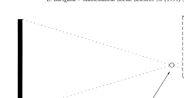
(i) The following figure illustrates a simple rule of geometric optics: if u (a unit in the observed reality) is an oblungate object lying perpendicular to the line of sight, then its length s and distance d from the nodal point of the eye and the length s9of its projection
u9 on the image plane (representing the retina) are related by the following equation:
s /d5s9/d9 (12)
where d9 is the separation of the nodal point from the image plane (see Fig. 2). This optical rule may be described as a constraintg, acting on variables at the S- and I-levels of data (it qualifies as an SI-constraint). Conditionmg states that three variables s, d, s9
Fig. 2. Simplified observational context for the size–distance invariance hypothesis.
(ii) The second example is offered by stereo vision, as it applies to very simple observational contexts, of the kind illustrated in Fig. 3. The terms to be considered are:
9 9
two linear vertical objects u and u in the physical scene, their projections u , u1 2 l 1 l 2 on
9 9
the left and u , ur1 r 2on the right image planes, egocentric distance d of the nearer object (u in this example), separation in depth e between the objects, binocular disparity b1 9of their retinal images (b9may roughly be identified with the difference between separation of images on the left retina and separation of images on the right retina). Optical analysis shows that, for a good approximation, the following equation holds true:
2
b9 5ie /(d 1de), (13)
where i is interpupillary distance. This equation may be thought of as thes-condition of an optical constraint, acting on S-variables d, e and I-variable b9; them-condition of the constraint specifies that three variables are involved; thet-condition qualifies variable d
as an egocentric distance, variable e as an exocentric distance, variable b9as a measure of binocular disparity; the l-condition defines correspondences between the units to which such quantities refer. Here too, besides the optical constraint, we might consider the psychophysical constraint which relates binocular disparity b9 to perceived egocen-tric distance d0 of the nearer object and perceived exocentric distance e0 between the objects, and assume the optical formula as a tentative model for thes-condition of the psychophysical constraint. In this way, from Eq. (13), through substitution of terms and inversion, the following formula is obtained:
2 99
e0 5b9d /(i2b9d0).
This formula is mentioned in the literature as a possible rule for perceptual estimation of depth separation between two objects, on the basis of perceived egocentric distance and binocular disparity (cf. Gogel, 1960; Ogle, 1962).
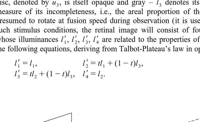
(iii) The third example refers to a rather different perceptual problem, i.e., the emergence of phenomenal achromatic transparency using an episcotister, as shown in Fig. 4. This figure represents an observational situation wherein the physical scene is comprised of a rectangular surface with an incomplete disc in front of it, both lying perpendicular to the line of sight. The rectangular surface is opaque and gray in colour, and divides into two parts u and u of different gray shades and of correspondingly1 2 different luminances, l1 and l , in the given illumination conditions. The incomplete2 disc, denoted by u , is itself opaque and gray – l denotes its luminance and t is the3 3 measure of its incompleteness, i.e., the areal proportion of the open sector – and is presumed to rotate at fusion speed during observation (it is used as an episcotister). In
9 9 9 9
such stimulus conditions, the retinal image will consist of four parts u , u , u , u ,1 2 3 4 9 9 9 9
whose illuminances l , l , l , l are related to the properties of the observed reality by1 2 3 4 the following equations, deriving from Talbot-Plateau’s law in optics (cf. Pirenne, 1962):
9 9
l15l ,1 l25tl11(12t)l ,3
9 9
l35tl21(12t)l ,3 l45l .2
By applying the suggested categories, this system of equations may be conceived as the
s-condition of an optical constraint; the m-condition for the constraint specifies that 9 9 9 eight variables are involved, thet-condition qualifies l , l , l as luminances, l , l , l ,1 2 3 1 2 3
9
l4 as illuminances and t as a proportion, the l-condition characterizes the general architecture of the observational context, such that the relevant variables are properly located. In the presumed situation, the prevailing perceptual result is a scene with a
99 99 99
rectangular opaque surface comprised of two parts, u1 and u , with different values l2 1 99
and l2 of phenomenal luminance (brightness); and a stationary, complete, transparent 99
disc u , which appears to be in front of the rectangular surface, and is qualified by a3 99
certain degree l3 of phenomenal luminance and a certain degree t0 of phenomenal transparency. By substituting these four P-variables to the corresponding S-variables in
99
the given optical equations, and solving for unknowns t0and l , the following formulae3 are obtained:
9 9 9 9
t0 5(l22l ) /(l3 12l )4
99 9 9 9 9 9 9 9 9
l3 5(l l1 32l l ) /(l2 4 12l21l32l ),4
which correspond to Metelli’s equations on phenomenal transparency (Metelli, 1970, 1974). This pair of formulae may be thought of as thes-condition of a psychophysical constraint (an IP-constraint), which is conjectured and abstractly determined on the basis of an optical principle (the s-condition of an SI-constraint).
The examples just described have been introduced to illustrate the following basic aspects of relational constraints: each located constraint refers to a definite set of variables (its field of action); constraints may be classified, at a primary level, by referring to the gnosiological kind of variables they involve (SI-constraints, IP-con-straints, etc.); each constraint is qualified by a certain predictive condition, which amounts to a relation between possible values of the variables in the field of action; this predicted relation is conditional upon some specific premises concerning the number, type and location of the involved variables, so that a non-located constraint has the general shape of a formal implication. These are the aspects most important for the following analyses, but they certainly do not exhaust the complexity of the concept in question. Among other aspects and problems, let us mention the qualification of constraints according to the formal kind of variables they involve (dichotomous or categorical, possibly expressed by scales at some measurement levels, etc.); algebraic expressions of predictive conditions of constraints (in terms of equations, inequalities, logical formulae, etc.); requirements and procedures for empirical testing of relational constraints, as hypothetical empirical laws; and, last but not least, ways of arriving at conjectural constraints which are potentially relevant for vision. Let us briefly comment on this last issue, specifically referred to the production of conjectural psychophysical constraints (hypothetical IP-constraints).
basically for the sake of convenience: our purpose was to illustrate concisely both SI-and IP-constraints, using examples in which predictive conditions are expressed by simple equations. But now some qualifications are in order, on this specific point.
First: The method of transposition, as a direct way of producing conjectural psychophysical constraints based on known optical constraints, is not uncommon in visual science (various significant examples, taken from both the psychology of visual perception and computer vision, are analytically discussed in Burigana, 1999). This method may be viewed as part of a more general heuristic attitude in the study of vision, sometimes called ‘‘vision is inverse optics’’ (cf. Poggio et al., 1985). Second: The method of transposition is simply one of a variety of procedures used by researchers for determining conjectural dependence relations involving perceptual variables: psycho-physical constraints may also be conjectured or verified by combining or modifying constraints previously derived through transposition, or by applying procedures which are totally independent of optical analogies (see next paragraph). As regards the model proposed here, distinctions relating to the origin of various constraints are not of primary importance: a system of constraints, as defined in the next section, may be heteroge-neous in this respect, in that it comprises psychophysical constraints that are conceived or verified by means of different procedures. Third: The method of transposition, which appears so simple in execution – physical variables in an optical formula are substituted by their perceptual counterparts – is in fact a cumbersome and questionable operation, in the scientific view, since it results in transferring a regularity from one scientific level to another scientific level. This transfer operation is not illegitimate in an absolute sense but, in order to be accepted as plausible, it generally requires strong assumptions concerning structural similarities and correspondences of data between the two scientific levels (an analysis of assumptions implicit in some applications of the method is made in Burigana, 1999, Ch.3).
We conclude this discussion by referring to one alternative way of establishing constraints involving perceptual variables, which is quite different from the transposition method, and is well illustrated by Lukas (1987). The problem in this application regards perceptual constancy of size, and refers to observational contexts of the kind we considered in example (i) concerning the size–distance invariance hypothesis. Spe-cifically, it is presumed that a set O5ho , . . . , o1 njof observational cases similar to that in Fig. 2 is given, and that each case o (for jj 51, . . . , n) may be described as a pair (d ,j
9 9
s ), d being the egocentric physical distance of the oblungate object in the scene and sj j j
the visual angle corresponding to that object (the visual angle is closely related to the length of the retinal projection). Further, it is presumed that a binary relation R is determined on set O through psychological experimentation, where o Ro (for 1j l #j, l#n) means that the object in case o perceptually appears to the observer at least asj
long as the object in case o . Then, for empirical relational system (O, R), a possiblel
‘‘additive model of size constancy’’ is considered, which formally consists of three 9 positive real-valued functions f, g, h, so that: o Ro iff h(o )j l j $h(o ), h(o )l j 5g(d )f(s ) forj j
all 1#j, l#n. Reference is made to the theory of ‘‘additive conjoint measurement’’,
There are considerable differences between this approach, which is inspired by the representational measurement theory, and the traditional way of discussing the relation between perceptual size and perceptual distance, which we applied in example (i). These differences regard the empirical base (given by relation R of perceptual comparison, in this alternative approach), numerical expression of data (according to measurement scales f, g, h, in the new approach), conditions for validity of the model (i.e., assumptions for the legitimacy of a transposition, or formal requirements of relation R), possibilities and procedures for empirical testing of the model, and so on. We point out, in particular, that if functions h and g are interpreted as measures of the perceptual size and perceptual distance of objects in the observational cases, then equation h(o )j 5
9
g(d )f(s ) qualifying the ‘‘additive model of size constancy’’ is structurally similar toj j
equation s0 5d0s9d9 expressing the size–distance invariance hypothesis. This is a constraint involving perceptual variables which, in the way used by Lukas (1987), is independently obtained as the solution of a representational measurement problem, not as the result of a copying operation on an optical regularity, i.e., not as the result of a transposition procedure.
4. Systems of constraints
In the Introduction, the following circumstance was emphasized: in addressing perceptual problems on articulated observational contexts, several dependence relations must be considered, as a rule, which are potentially relevant for their solutions. This notion is now formalized into the concept of a system of constraints, defined as a set of located constraints and abstractly described by the following equation:
C5hc , . . . , c1 nj5h(g1,W ), . . . , (1 gn, W ) .n j
In other words, a system of constraints C is a set of instantiations of non-located constraintsg1, . . . ,gn on specific locations W , . . . , W within the presumed exhaustive1 n
set V of located variables. We emphasize again that system C may comprise constraints of various kinds (SI-, IP-, P-constraints, etc.), as well as separate instantiations of one type on distinct locations in V (this means that there may be repetitions along the list
g1, . . . , gn of the types of constraints constituting C ). System C may be depicted as a hypergraph on m nodes with n hyperedges (Berge, 1973): the nodes correspond to the variables in V and the hyperedges represent the constraints in C, as relations on definite subsets of variables. This representation resembles that used in AI to describe a ‘‘network of constraints’’ (cf. Montanari and Rossi, 1991; Gyssens et al., 1994). In fact, our definition of a system of constraints, specifically referred to perceptual problems, is abstractly similar to that of a network of constraints, as it is applied to a variety of computational problems in AI (belief maintenance, scheduling, logic programming, temporal reasoning, etc.; cf. Dechter, 1992; Kumar, 1992; Tsang, 1993).
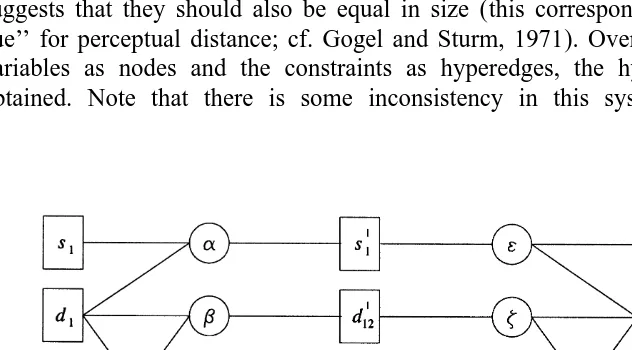
Units: Let u , u , u denote the rectangle on the left, the circle in the centre and the1 2 3
9 9 9 99 99
rectangle on the right, as items at the S-level of data; similarly, let u , u , u and u , u ,1 2 3 1 2 99
u3 denote the corresponding units at the I- and P-levels of data. We have already noted that, in the special kind of observational cases of the example, exact correspondence is presumed between the units at the three levels of data, i.e., there is no distortion concerning the number or identity of the units. Variables: At the S-level, let s ,s ,s be1 2 3 the geometrical sizes of objects u , u , u , and d , d , d their physical distances from1 2 3 1 2 3
9 9 9
the observer. At the I-level, for 1#i±j#3, let s be the size of projected unit u and bi i ij
9 9 99 99
the binocular disparity associated to projected units u and u . At the P-level, let s , s ,i j 1 2
99 99 99 99
s3 be the phenomenal sizes and d , d , d1 2 3 the phenomenal egocentric distances of 99 99 99
units u , u , u . Constraints: For the presumed kind of observational cases, both a set1 2 3 of SI-constraints and a set of IP-constraints may be considered. The former, for
9 9
1#i±j#3, includes an optical constrainta(s , d , s ) which relates the size of I-unit ui i i i
to the size and distance of the corresponding S-unit u , and an optical constrainti
9 9 9
b(d ,d ,b ) which derives the binocular disparity between I-units u , ui j ij i j from the distances of S-units u , u . The latter, for 1i j #i±j#3, includes a psychophysical
9 99 99
constraint e(s , s , d ) (a version of the size–distance invariance hypothesis) whichi i i
99 connects the phenomenal size and phenomenal egocentric distance of P-unit ui to the
9 9 99 99
size of the associated I-unit u , and a psychophysical constrainti z(b , d , d ) whichij i j
99 99
connects the phenomenal egocentric distances of P-units u , ui j to the binocular
9 9 99 99
disparity of the corresponding I-units u , u . In addition, a P-constrainti j h(s , s ) may be1 3
99 99
conjectured: it is promoted by the equality in shape between units u1 and u , and3 suggests that they should also be equal in size (this corresponds to the ‘‘relative size cue’’ for perceptual distance; cf. Gogel and Sturm, 1971). Overall, by representing the variables as nodes and the constraints as hyperedges, the hypergraph in Fig. 5 is obtained. Note that there is some inconsistency in this system of constraints, as
9 99 99 99 99 99 99
constraint z(b , d , d ) supports d13 1 3 1 .d , while constraint3 h(s , s ), combined with1 3
9 99 99 9 99 99 99 99
e(s , s , d ) and1 1 1 e(s , s , d ), favours d3 3 3 1 ,d .3
Coming back to general aspects, we note that the overall predictive power of a system of constraints C5hc , . . . , c1 njmay be adequately represented in extension E(C ), which is the set of complete valuations that satisfy the predictions of all constraints in C, i.e.:
E(C )5hx[X: x[E(c ), . . . , x1 [E(c )n j
5E(c )1 > ? ? ?>E(c ).n
This is exactly the analogue of the set of ‘‘admissible solutions’’ for a ‘‘constraint satisfaction problem’’ (Mackworth, 1992), and of the set of ‘‘consistent labelings’’ for a ‘‘relaxation labeling problem’’ (Hummel and Zucker, 1983). Since C is defined as a set of located constraints, one presumes that, for each cj5(gj, W )j [C, premisesmj,tjand
lj of typegj are satisfied by W on each observational case oj [O; if (as expected) the
same is true for predictive conditions sj ( j51, . . . , n), then we should have V(o)[
E(C ) for all o[O, i.e.:
V(O )#E(C ). (14)
In other words, the set of joint values taken on by variables in V on cases in O should be included in the extension of the system of constraints.
This is the formal expectation of the model, which in practice may prove not to be exactly true. In fact, constraints are here conceived as kinds of scientific hypotheses: they are conjectural predictive regularities on perceptual processes, to be tested and refined through experimentation. What is more, constraints are regularities which apply locally to restricted subsets of the general set of variables, and to selected portions of the spatio-temporal extent of the observational cases. Thus, it may happen that each constraint in C, in isolation, is a plausible rule, but system C as a whole is not consistent (in this respect, constraints are like the local principles of geometric coherence in impossible figures; cf. Sugihara, 1982; Kulpa, 1987). For these reasons, the prediction of Eq. (14) may not be confirmed. It is possible that E(C )±[ but V(O ),⁄ E(C ), in which case system C would prove to be formally consistent (there is some complete valuation which complies with all constraints in C ), but some observational cases disagree with some predictions of constraints in C. More strongly, it is possible that E(C )5[(which obviously implies V(O ),⁄ E(C )), in which case system C would be formally inconsistent, i.e., at some points some predictive conditions of constraints in C conflict with one other, so that no complete valuation can obey all the constraints in the system.
The latter possibility is significant for theoretical analysis, since it characterizes the ‘‘cue conflict paradigm’’ frequently used in perceptual research. This issue will be examined more closely in Section 6. In cases of inconsistency of system C, consistency may be restored by ignoring some of its constraints; this means that only selected subsystems of C are considered. The predictive power of any subsystem D5hc , . . . ,j1
cjpj#C is expressed by its extension:
which is the set of complete valuations complying with all constraints in D. It is immediately seen that, for all D, D9#C:
if D#D9, then E(D )$E(D9) (16)
E(D<D9)5E(D )>E(D9). (17)
Consistent subsystems are subsets of C with non-empty extensions; Eq. (16) shows that the set of consistent subsystems is an order ideal in the power-set of system C.
5. Pairing of constraints and valuations
The specific phenomenal scene an observer perceives in a given observational situation may be interpreted as the result of two complementary classes of factors: a network of relational rules, which instantiate some general principles of conditioning and interaction, and a set of input data, which are offered by and strictly contingent upon that particular situation. In our theoretical frame, the former class of factors are represented as an extensive system C of located constraints, while the latter class may be described as a (partial) valuation y which specifies the values taken on by some set of S- and / or I-variables (stimulus variables) in the presumed observational situation. On a similar basis, Clark and Yuille (1990) distinguish between ‘‘a priori (scene independent) constraints’’ and ‘‘scene dependent sources of information’’ (p.158). We note, however, that in our view located constraints are themselves ‘‘scene dependent’’ to some extent, in that each constraint cj5(gj, W ) acts on a definite set Wj j#V of located variables, which
is supposed to satisfy premises mj,tj and lj of typegj.
Thus, we are led to consider any pairing (C, y) between the presumed system of constraints C and some valuation y on a set of S- and / or I-variables. More generally, for the needs of formal analysis, we may refer to any pairing (D, Z ) between some subsystem of constraints D#C and some subset of valuations Z#Y. To each pairing
(D, y), with D#C and y[Y, an extension E(D, y) is associated, which is the set of
complete valuations that are compatible with valuation y and comply with all constraints in D. In other words, the extension of a pairing is the intersection of the extensions of its components (as they are defined by (4) and (15)), i.e.:
E(D, y)5E(D )>E( y). (18)
More generally, for each D#C and Z#Y, we define:
E(D, Z )5E(D )>E(Z ), (19)
i.e., the extension of pairing (D,Z ) is the set of complete valuations which are compatible with some valuations in Z and comply with all constraints in D; equivalently:
E(D, Z )5 <y[ZE(D, y).
C X
C Y X C Y X
mapping of 2 32 in 2 (2 , 2 and 2 are the power-sets of sets C, Y and X ). The following formulae show some elementary properties of these mappings:
if D#D9and y#y9, then E(D, y)$E(D9, y9) (20)
if y↔y9, then E(D<D9, y<y9)5E(D, y)>E(D9, y9) (21)
in view of (5), (16), (7) and (17). In addition:
if D#D9and Z$Z9, then E(D, Z )$E(D9, Z9)
E(D<D9, Z )5E(D, Z )>E(D9, Z )5E(D9, E(D, Z )) (22)
E(D, Z<Z9)5E(D, Z )<E(D, Z9)
E(D, d(Z, Z9))5E(D, Z )>E(D, Z9) (23)
because of (6), (16), (17), (8) and (9). Eqs. (21), (22) and (23) show that the ranges of
X
mappings (18) and (19) within power-set 2 are closed to intersection (i.e., they are closure systems), provided that E(C ) is a proper subset of X.
The consistency of a system of constraints may now be redefined in a relative form with respect to a partial valuation. That is, any subsystem of constraints D#C is said to
be consistent with a given valuation y[Y if E(D, y)±[, i.e., when there is at least one complete valuation that includes y and complies with all constraints in D. In view of remarks in the previous paragraphs about the joint action of a system of constraints and a set of input data in the construction of a perceptual scene, it is the relative concept of consistency which really matters in formal analysis. Any subsystem of constraints is absolutely inconsistent (in the sense defined in Section 4) if and only if it is inconsistent with respect to all valuations in Y. Moreover, it may be directly inferred from Eq. (20) that, for all D, D9#C and y, y9[Y:
if D$D9, y$y9, and D is consistent with y, then D9is consistent with y9.
This property means that, for any fixed valuation y, the set of all subsystems of
C
constraints consistent with y is an order ideal in power-set 2 , the order ideal being completely determined by its maximal members, which are the maximal consistent
subsystems with respect to valuation y. If the complete system C is inconsistent with a
given set of input data y, then each maximal consistent subsystem represents the result of a minimal reduction of C, such that consistency with y is achieved. Such subsystems have the following properties, which result directly from Eq. (21):
if D is a maximal consistent subsystem with respect to y and c[C2D,
then E(c)>E(D, y)5 [;
if D±D9are maximal consistent subsystems with respect to y,
then E(D, y)>E(D9, y)5 [. (24)
coordinates whose values are uniquely determined by the joint action of D and y. This set will be denoted as F(D, y) and is formally specified by the following equation:
F(D, y)5hi[M: p (E(D, y), i )u u51 ,j
where p is the projection operation given in (3). The definition itself implies that, for each consistent pairing (D, y):
F(D, y)$Muy.
Property (20) also ensures that, for all consistent pairings (D, y), (D9, y9):
if D#D9and y#y9, then F(D, y)#F(D9, y9).
Let us assume that valuation y describes a set of input data (i.e., an assignment of values to some stimulus variables), which is the most natural presumption in our perspective. Each P-variable in the set of variables VuF(D, y) thus represents a perceptual aspect
unambiguously determined or ‘‘specified’’ by input data in y combined with constraints in D, while any P-variable in V2VuF(D, y) preserves some uncertainty, in that it admits
two or more distinct values in spite of the joint constraining action of y and D. Of course, a perfect model would consist of a system of constraints C which is absolutely consistent and such that F(C, y)5M for all valuations y on a suitable set of independent
stimulus variables.
6. Constraints in perceptual science
In the next paragraphs we will discuss in greater detail the plausibility and possible use of the multiple constraint paradigm (MCP) in the theory of visual perception. This section of the paper will thus resume and work out the suggestions given in the Introduction, in which MCP was qualified as a possible way of conceptualizing the complex state of affairs in the study of visual phenomena.
variables. For any observational case o[O, pairing (C, W ) is a consistent model if E(C, W(o))±[, a sufficient model if F(C, W(o))5M, and a faithful model if E(C, W(o))5
V(o) ; in other words, a model is faithful for a certain observational case if it
h j
unambiguously predicts the values actually taken on by all variables (in particular, perceptual variables) in that specific case.
Reference to MCP also may help in explaining some terms of the multi-factor ¨
approach to vision, such as the ‘‘mutual disambiguation’’ of stimulus cues (Bulthoff and Mallot, 1990; Landy et al., 1995), ‘‘over-specification’’ and ‘‘under-specification’’ of a perceptual content (Massaro, 1988). For example, if variables v and v represent
i9 i0
stimulus aspects which separately influence some P-variable v, then the mutual
i
disambiguation ofv andv in a given observational case o may mean the following:
i9 i0
projection p(E(C, (i9, s (o)), (ih 0, s (o)) ), i ) (i.e., the set of values admissible forj v that
i9 i0 i
is defined by the assignment of values s (o), s (o) to variablesv ,v , and by constraints
i9 i0 i9 i0
in C ) is smaller than projections p(E(C, (ih 9, s (o)) ), i ) and p(E(C, (ii9 j h 0, s (o)) ), i ).i0 j
Further, ifv is a specific perceptual variable and W5hv , . . . ,v jis a set of stimulus
i i1 ik
variables, then to state that W under-specifiesv in some observational case o means that
i
p(E(C, W(o)), i )$2 (i.e., input data in W(o) together with constraints in C are not
u u
strong enough to reduce the set of values admissible forv to a singleton, so that model
i
(C,W(o)) is not sufficient relative to variablev). Similarly, to state that W over-specifies
i
Theories on visual perception may include process-like implications, in which some steps are supposed to precede other steps, or some factors are presumed to act on situations prepared by other factors. This dynamic (or genetic) side of perceptual theorization clearly appears in the use of expressions such as ‘‘propagation of disambiguation’’ (Marr, 1982, p.141), ‘‘cue promotion’’ (in the so-called ‘‘modified weak fusion model’’; cf. Landy et al., 1995), ‘‘perceptual causation and interaction’’ (Gogel, 1973; Epstein, 1982), and so on. MCP is generally compatible with such dynamic implications of perceptual science: in explaining the composition of a perceptual scene, some priorities may be hypothesized between multiple constraints, i.e., some constraints may be presumed to act before and prepare the action of others. Eq. (22) exemplifies a type of formal result which may be useful in this perspective. It implies, by iteration, that E(D, y)5E(c , E(cjp jp21, . . . , E(c , y) . . . )) for any set ofj1
constraints D5hc , . . . , cj1 jpj#C and any valuation y[Y, i.e., the overall predictive
power of a set of constraints D may be expressed progressively, through successive exploitation of the single constraints making up the set.
aspect, support two quite different values for that aspect. This is sometimes called the
cue conflict paradigm (Blake et al., 1993; Buckley and Frisby, 1993). The method serves
at least two important scientific purposes: first, it is used to estimate the relative strength of different stimulus factors for a fixed perceptual aspect; second, it allows us to explore the rules of combination or interaction of the effects of those different factors. The cue conflict paradigm has been widely used in recent research on perceptual recovery of solid shapes and distances from multiple cues to depth; in particular, it is the basis of the so-called ‘‘perturbation analysis’’ applied to the study of such perceptual phenomena (Maloney and Landy, 1989; Young et al., 1993; Landy et al., 1995). But this paradigm has a very long tradition in perceptual science: it is found, for example, in some of the figural cases discussed by Wertheimer (1923), in which the strength of different factors of perceptual grouping is comparatively estimated by orienting their effects in opposite directions.
Within MCP, a conflictual visual context may be described as an observational case o, such that the system of constraints C acting in it is not consistent with valuation W(o) of a selected set W#V of stimulus variables. The inconsistency is due to the fact that
distinct parts W9(o), W0(o) of W(o) specify different values for a fixed P-variablev [V
i
by means of constraints in C, so that no complete valuation on V can include W(o) and at the same time comply with all constraints in C. By pursuing the set-theoretic approach, we may conjecture that, in a conflictual case o, the perceptual system will ignore some constraints in C (and the data in W(o) which are involved only in those constraints), and will operate on some subsystem D#C which is maximal consistent with W(o). Because
of Eq. (24), experimentation should make it possible to identify the maximal consistent subsystem preferred by the visual system, and thus to evaluate the relative importance of the various constraints in C and input data in W(o).
This refinement of MCP is closely connected with the set-theoretic approach, in that the additional assumptions deal with operations of a selective type: the selection of a maximal consistent subsystem of constraints, and possibly also that of a complete valuation in its extension (if the chosen subsystem is not formally sufficient). Similar ideas may be found in some contemporary theoretical assumptions: for example, the ‘‘vetoing hypothesis’’ or the ‘‘winner-take-all principle’’ as applied to vision with
¨
conflictual stimulus data (Bulthoff and Mallot, 1988; Clark and Yuille, 1990, §3.3; Johnston et al., 1993). There are other plausible ways of theorizing about perceptual processing in conflictual contexts. One may conjecture, for example, some ‘‘combination rule’’ (in the form of a weighted sum, an average, a multiplication, etc.) which uniquely determines the value of a perceptual variable by combining different values supported for that variable by separate parts of the input data (cf. Bruno and Cutting, 1988; Maloney and Landy, 1989; Young et al., 1993). But these developments, which involve operations on numerical values, are not typical of a pure set-theoretic approach.
Lastly, we must point out the significance of MCP in analysing multiple visual
illusions, i.e., perceptual phenomena in which various contents in the perceptual scene
the joint variability of several perceptual features in a bistable figure (Necker’s cube, Rubin’s examples on figure–ground inversion, etc.; cf. Attneave, 1971; Rock et al., 1994). In a multiple illusion, distinct perceptual errors appear to be mutually dependent, according to principles of complementarity: for a fixed observed reality, errors concerning some perceptual properties must be compensated by errors on other perceptual properties, so that the perceptual scene as a whole is compatible with the given set of stimulus conditions. Now, such a situation may be represented as a network of P-constraints deriving from proper SP- or IP-constraints through sectioning opera-tions: a psychophysical constraint which involves two or more perceptual variables gives rise to regular dependence at the perceptual level, if the stimulus data are fixed and variations are induced in some of the involved perceptual variables. Multiple illusions are commonly regarded as highly significant situations in the study of the rules of perceptual organization.
7. Epilogue: reasons for the set-theoretic approach
The framework presented in this paper is set-theoretic in nature, in that its formal components are solely grounded in concepts from set theory. What are the reasons for this choice? What are the expected benefits of the set-theoretic approach in treating problems in the science of vision? Comments in this last section are intended to provide some answers to these questions.
We conceive set theory as a basic language particularly suitable for defining plain, flexible scientific models, i.e., models with a minimum of requirements of the real contexts or problems to which they may be applied. Contemporary investigation on the interaction of factors in human and machine vision resorts to various formal and computational paradigms (fusion models, regularization theory, theory of Markov fields, etc.) which, in some applications, result in highly complex models with selective requirements. Instead, we need a theoretical framework with a minimum of primitive terms and assumptions. The first reason is that we intend to show that a variety of important concepts currently used by researchers on vision may in fact be made explicit with a relatively simple set of general prerequisites. This demonstration was done in the previous section. We do not mean, of course, that all formal developments in modern visual science may be grounded on a purely set-theoretic platform (we have just mentioned, for example, the elementary concept of a ‘‘combination rule’’ relating to the cue conflict problem, which cannot be directly located within the proposed framework). What is meant here is that a relatively simple network of assumptions is sufficient to support the rigorous definition of some crucial and representative concepts in modern visual science.
accommodation, convergence, binocular disparity, occlusion, motion parallax, etc.), each factor being qualified by a certain mode of action in conditioning the perceptual result. But there are, in general, conspicuous qualitative differences between factors (some are optico-geometric quantities, others relational conditions, yet others dichotomous vari-ables, etc.), between corresponding rules of action (some are expressed by equations, others may be represented as logical formulae) and between the kinds of information provided by the factors (concerning distance from the subject, distance between objects, or simply the order in the third dimension; cf. Cutting and Vishton, 1995). In dealing with a composite problem of this sort, it is in fact impossible to represent the whole structure in terms of a specialized calculus (e.g., as a system of numerical equations on variables which are all quantitative, or as a system of logical formulae on variables which are all dichotomous, etc.). So we are forced to look for a comprehensive basic calculus constituting a common platform for all the various terms in the problem: that calculus is here identified with set theory. Based on this choice, the contribution of each factor is represented as a subset of a common space (i.e., an extension in the universe of complete valuations; cf. Sections 2 and 3), and interactions between factors are described and analysed in terms of relations and operations (inclusion, intersection, restriction, etc.) between such subsets.
Somehow related to this argument is a property inherent in the concept of a pairing (C, W(o)) between a system of constraint C and valuation W(o) of a set of stimulus variables W in an observational case o (cf. Sections 5 and 6). In a sense, both C and
W(o) are sources of information which take part in determining the perceptual result: the
former is a normative source (a system of rules), the latter a source strictly contingent upon the presumed observational case. Within the suggested framework, the information-al contributions of both sources are represented in a uniform way, as subsets E(C ) and
E(W(o)) of universe X of complete valuations, and their combined effect is described as
the intersection E(C, W(o))5E(C )>E(W(o)) of the two subsets.
One further perspective for an appreciation of the suggested set-theoretic approach concerns its possible analysis and development, as a mathematical construction. There are in the model some elements of structural substance which allow us to consider such a possibility. The model basically concerns systems of relations (constraints), acting locally on a large set of dimensions (variables); the relations are represented as subsets of the direct product of all dimensions, and may be subjected not only to ordinary Boolean operations (union, intersection, etc.) but also to the more specialized operations (restriction, disjunction, projection, etc.) defined in Section 2. Properties and implications of such a composite system of operations constitute the matter for a possible formal investigation. In particular, systems of relations are here represented as families of subsets of a common general space, and this fact suggests the opportunity of exploring the algebraic properties of such set-theoretic structures. Some very short steps in this direction are made in Sections 2, 4 and 5, where we noted that certain families of sets defined there qualify as ‘‘lattices’’, ‘‘closure systems’’ or ‘‘order ideals’’. These are small particles of an abstract algebraic investigation, which seems to us worthy of being carried out.
dimension, grouping in the scene, organization of light and colours, etc.), the ultimate goal is to determine a valuation of the set of perceptual variables which is compatible with both the given valuation of the set of stimulus variables and the system of constraints presumed to be at work in the observational context. Substantially, this is a goal of scientific prediction and resembles the ‘‘constraint satisfaction problem’’ considered in the field of artificial intelligence: given a ‘‘network of constraints’’ on a set of variables, find an assignment of values to the variables so that it complies with all constraints in the network. Referring to various specifications of such a general problem, researchers in information sciences and artificial intelligence have developed a variety of algorithms and computer programs for finding single solutions or sets of alternative solutions (cf. Tsang, 1993). In principle, these computational resources are also available for dealing with problems of integration of visual factors, provided that they may be formulated in the suggested set-theoretic terms.
Acknowledgements
The author wishes to express his sincere thanks to one anonymous referee, for constructive criticisms and useful suggestions on previous versions of the paper. He also thanks Ms Gabriel Walton, for revision of the English text.
References
Aloimonos, J., Shulman, D., 1989. Integration of Visual Modules. An Extension of the Marr Paradigm, Academic Press, New York.
Attneave, F., 1971. Multistability in perception. Scientific American 225 (6), 62–71.
Balzer, W., Moulines, C.U., Sneed, J.D., 1987. An Architectonic for Science. The Structuralist Program, Reidel Publishing, Dordrecht.
Berge, C., 1973. Graphs and Hypergraphs, North-Holland, Amsterdam. ¨
Blake, A., Bulthoff, H.H., Sheinberg, D., 1993. Shape from texture: Ideal observers and human psychophysics. Vision Research 33, 1723–1737.
Bruno, N., Cutting, J.E., 1988. Minimodularity and the perception of layout. Journal of Experimental Psychology: General 117, 161–170.
Buckley, D., Frisby, J.P., 1993. Interaction of stereo, texture and outline cues in the shape perception of three-dimensional ridges. Vision Research 33, 919–933.
¨
Bulthoff, H.H., 1991. Shape from X: Psychophysics and computation. In: Landy, M.S., Movshon, J.A. (Eds.), Computational Models of Visual Processing, MIT Press, Cambridge, MA, pp. 305–330.
¨
Bulthoff, H.H., Mallot, H.A., 1988. Integration of depth modules: Stereo and shading. Journal of the Optical Society of America A 5, 1749–1758.
¨
Bulthoff, H.H., Mallot, H.A., 1990. Integration of stereo, shading and texture. In: Blake, A., Troscianko, T. (Eds.), AI and the Eye, Wiley, New York, pp. 119–146.
Burigana, L., 1999. From Optical to Visual Relational Constraints. Basic Concepts and Selected Examples, Guerini e Associati, Milano.
Clark, J.J., Yuille, A.L., 1990. Data Fusion for Sensory Information Processing Systems, Kluwer Academic, Boston, MA.