Contents lists available atScienceDirect
Journal of Econometrics
journal homepage:www.elsevier.com/locate/jeconom
Dynamic estimation of volatility risk premia and investor risk aversion from
option-implied and realized volatilities
✩Tim Bollerslev
a,b,c,∗, Michael Gibson
d,1, Hao Zhou
d,2 aDepartment of Economics, Duke University, Post Office Box 90097, Durham NC 27708, USA bNBER, USAcCREATES, Denmark d
Risk Analysis Section, Federal Reserve Board, Mail Stop 91, Washington DC 20551, USA
a r t i c l e i n f o
Article history:
Available online 6 March 2010
JEL classification:
G12 G13 C51 C52
Keywords:
Stochastic volatility risk premium Model-free implied volatility Model-free realized volatility Black–Scholes
GMM estimation Return predictability
a b s t r a c t
This paper proposes a method for constructing a volatility risk premium, or investor risk aversion, index. The method is intuitive and simple to implement, relying on the sample moments of the recently popularized model-free realized and option-implied volatility measures. A small-scale Monte Carlo experiment confirms that the procedure works well in practice. Implementing the procedure with actual S&P500 option-implied volatilities and high-frequency five-minute-based realized volatilities indicates significant temporal dependencies in the estimated stochastic volatility risk premium, which we in turn relate to a set of macro-finance state variables. We also find that the extracted volatility risk premium helps predict future stock market returns.
©2010 Elsevier B.V. All rights reserved.
1. Introduction
Two new model-free volatility measures have figured promi-nently in the recent academic and financial market practitioner literature. ‘‘Model-free realized volatilities’’ are computed by sum-ming squared returns from high-frequency data over short time
✩ The work of Bollerslev was supported by a grant from the National Science
Foundation to the NBER and CREATES funded by the Danish National Research Foundation. We would also like to thank three anonymous referees, Alain Chaboud, N.K. Chidambaran, Hui Guo, George Jiang, Chris Jones, Nellie Liang, Nour Meddahi, Nagpurnanand R. Prabhala, Patricia White, and seminar participants at the Venice Conference on Time-Varying Financial Structures 2005, the Federal Reserve Conference on Financial Market Risk Premia 2005, Peking University, the Bank for International Settlement, and the AFA 2006 Annual Meeting for useful comments and suggestions. The views presented here are solely those of the authors and do not necessarily represent those of the Federal Reserve Board or its staff. Matthew Chesnes and Stephen Saroki provided excellent research assistance.
∗Corresponding author at: Department of Economics, Duke University, Post Office Box 90097, Durham NC 27708, USA. Tel.: +1 919 660 1846; fax: +1 919 684 8974.
E-mail addresses:[email protected](T. Bollerslev), [email protected](M. Gibson),[email protected](H. Zhou).
1 Tel.: +1 202 452 2495; fax: +1 202 728 5887. 2 Tel.: +1 202 452 3360; fax: +1 202 728 5887.
intervals during the trading day. As demonstrated in the literature, these types of measures afford much more accurate ex post obser-vations of actual volatility than the more traditional sample
vari-ances based on daily or coarser frequency data (Andersen et al.,
2001;Barndorff-Nielsen and Shephard, 2002;Meddahi,2002;
An-dersenet al.,forthcoming,2003;Barndorff-Nielsen and Shephard, 2004a;Andersen et al.,2004). ‘‘Model-free implied volatilities’’ are computed from option prices without the use of any
partic-ular option-pricing model. These measures provide ex ante
risk-neutralexpectations of future volatilities and do not rely on the
Black–Scholes pricing formula or some variant thereof (Carr and
Madan, 1998;Demeterfi et al.,1999;Britten-Jones and Neuberger, 2000;Lynch and Panigirtzoglou, 2003;Jiang and Tian, 2005;Carr and Wu, 2009).3In this paper, we combine these two new
volatil-3 Market participants have also recently developed several new products – realized variance futures, VIX futures, and over-the-counter (OTC) variance swaps – that are based on these two model-free volatility measures. Specifically, the Chicago Board Option Exchange (CBOE) recently changed its implied volatility index (VIX) to use the model-free implied volatility approach and the more popular S&P500 index options (CBOE Documentation, 2003), while the CBOE Futures Exchange began to trade futures on the VIX on March 26, 2004 and realized variance futures on the S&P500 on May 18, 2004.Demeterfi et al.(1999) discuss OTC variance swaps. 0304-4076/$ – see front matter©2010 Elsevier B.V. All rights reserved.
ity measures to improve on existing estimates of the risk premium associated with stochastic volatility risk and investor risk aversion. Because the method we present here directly uses the model-free realized and implied volatilities to extract the stochastic volatility risk premium, it is easier to implement than other methods which rely on the joint estimation of both the underlying asset return and the price(s) of one or more of its derivatives, which requires complicated modeling and estimation procedures (see, e.g., Bates, 1996;Chernov and Ghysels, 2000; Jackwerth,2000;
Aït-Sahalia and Lo, 2000;Benzoni,2002;Pan,2002;Jones,2003;
Eraker,2004;Aït-Sahalia and Kimmel, 2007, among many others). In contrast, the method of this paper relies on standard GMM estimation of the cross conditional moments between risk-neutral and objective expectations of integrated volatility to identify the stochastic volatility risk premium. As such, the method is simple to implement and can easily be extended to allow for a time-varying volatility risk premium. Indeed, one feature of our estimation strategy is that it allows us to capture time-variation in the volatility risk premium, possibly driven by a set of economic state variables.4
The closest paper to ours is Garcia et al. (forthcoming),
who estimate jointly the risk-neutral and objective dynamics, using a series expansion of option-implied volatility around the Black–Scholes implied volatility. This approach has the advantage of relying on only a single option price to identify the risk premium parameter, while our approach requires a large number of option prices to construct the model-free implied volatility measure. On the other hand, model-free implied volatility effectively aggregate out some of the pricing errors in individual options, which may
adversely affect the series expansion approach. Garcia et al.
(forthcoming) also bring in higher order moments of the integrated volatility (skewness in particular) to identify the underlying dynamics, beyond the first two conditional moments explored by
Bollerslev and Zhou(2002).
To validate the performance of the new estimation strategy, we perform a small-scale Monte Carlo experiment focusing directly on our ability to precisely estimate the risk premium parameter. While the estimation strategy applies generally, the Monte Carlo
study focuses on the popularHeston(1993) stochastic volatility
model. The results confirm that using model-free implied volatility from options with one month to maturity and realized volatility from five-minute returns, we can estimate the volatility risk premium nearly as well as if we were using the actual (unobserved and infeasible) risk-neutral implied volatility and continuous time integrated volatility. However, the use of Black–Scholes implied volatilities and/or realized volatilities from daily returns generally results in biased and inefficient estimates of the risk premium parameter, leading to unreliable statistical inference.
To illustrate the procedure empirically, we apply the method to estimate the volatility risk premium associated with the S&P500 market index. We extend the method to allow for time variation in the stochastic volatility risk premium. We allow the premium to vary over time and to depend on macro-finance state variables. We find statistically significant effects on the volatility risk premium from several macro-finance variables, including the market volatility itself, the price-earnings (P
/
E) ratio of the market, a measure of credit spread, industrial production, housing starts,the producer price index, and nonfarm employment.5
Our results give structure to the intuitive notion that the difference between implied and realized volatilities reflects a
4 The general strategy developed here is also related to the literature on market-implied risk aversion (see, e.g.,Jackwerth,2000;Aït-Sahalia and Lo, 2000; Rosenberg and Engle, 2002;Brandt and Wang, 2003;Bliss and Panigirtzoglou, 2004; Gordon and St-Amour, 2004). A recent paper byWu(2005) also uses model-free realized and implied volatilities to estimate a flexible affine jump-diffusion model for volatility under the risk-neutral and objective measures.
5 For directly traded assets like equities or bonds, empirical links between the risk premium – expected excess return – and macro-finance state variables are
volatility risk premium that responds to economic state variables. As such, our findings should be of direct interest to market participants and monetary policymakers who are concerned with the links between financial markets and the overall economy. Further broadening our results, we also find that the estimated time-varying volatility risk premium predicts future stock market returns better than several established predictor variables.
The rest of the paper is organized as follows. Section2outlines the basic theory behind our simple GMM estimation procedure,
while Section3provides finite sample simulation evidence on the
performance of the estimator. Section4applies the estimator to
the S&P500 market index, explicitly linking the temporal variation in the volatility risk premium to a set of underlying macro-finance variables. This section also documents our findings related to return predictability. Section5concludes.
2. Identification and estimation of the volatility risk premium
Consider the general continuous-time stochastic volatility model for the logarithmic stock price process (pt
=
logSt),dpt
=
µ
t(
·
)
dt+
VtdB1t,
dVt
=
κ(θ
−
Vt)
dt+
σ
t(
·
)
dB2t,
(1)
where the instantaneous corr
(
dB1t,
dB2t)
=
ρ
denotes thefa-miliar leverage effect, and the functions
µ
t(
·
)
andσ
t(
·
)
mustsat-isfy the usual regularity conditions. Assuming no arbitrage and a linear volatility risk premium, the corresponding risk-neutral dis-tribution then takes the form
dpt
=
rt∗dt+
VtdB∗1t,
dVt
=
κ
∗(θ
∗−
Vt)
dt+
σ
t(
·
)
dB∗2t,
(2)
where corr
(
dB∗1t,
dB∗2t)
=
ρ
, andrt∗denotes the risk-free interest rate. The risk-neutral parameters in(2)are directly related to theparameters of the actual price process in Eq.(1)by the
relation-ships,
κ
∗=
κ
+
λ
andθ
∗=
κθ /(κ
+
λ)
, whereλ
refers to thevolatility risk premium parameter of interest. Note that the func-tional forms of
µ
t(
·
)
andσ
t(
·
)
are completely flexible as long asthey avoid arbitrage.
2.1. Model-free volatility measures and moment restrictions
The point-in-time volatilityVtentering the stochastic volatility model above is latent and its consistent estimation through filtering faces a host of market microstructure complications. Alternatively, the model-free realized volatility measures afford a simple approach for quantifying the integrated volatility over non-trivial time intervals. In our notation, let Vtn,t+∆ denote
the realized volatility computed by summing the squared high-frequency returns over the
[
t,
t+
∆]
time-interval:Vtn,t+∆
≡
n
−
i=1
pt+i
n(∆)
−
pt+i−n1(∆)
2.
(3)It follows then by the theory of quadratic variation (see, e.g.,
Andersen et al.(forthcoming), for a recent survey of the realized volatility literature),
lim
n→∞V n t,t+∆
a.s.
−→
Vt,t+∆≡
∫
t+∆t
Vsds
.
(4)In other words, whennis large relative to∆, the realized volatility should be a good approximation for the unobserved integrated volatilityVt,t+∆.6
Moments for the integrated volatility for the model in(1)have
previously been derived byBollerslev and Zhou(2002) (see also
Meddahi(2002) andAndersen et al.(2004)). In particular, the first conditional moment under the physical measure satisfies
E
(
Vt+∆,t+2∆|Ft)
=
α
∆E(
Vt,t+∆|Ft)
+
β
∆,
(5) where the coefficientsα
∆=
e−κ∆andβ
∆=
θ (
1−
e−κ∆)
are functions of the underlying parametersκ
andθ
of(1).Using option prices, it is also possible to construct a model-free measure of the risk-neutral expectation of the integrated volatility. In particular, let IV∗
t,t+∆ denote the time t implied
volatility measure computed as a weighted average, or integral, of
a continuum of∆-maturity options,
IV∗ t,t+∆
=
2∫
∞0
C
(
t+
∆,
K)
−
C(
t,
K)
K2 dK
,
(6)whereC
(
t,
K)
denotes the price of a European call option maturingat time t with strike price K. As formally shown by
Britten-Jonesand Neuberger (2000), this model-free implied volatility
then equals the true risk-neutral expectation of the integrated volatility,7
IV∗
t,t+∆
=
E∗
Vt,t+∆|Ft
,
(7)where E∗
(
·
)
refers to the expectation under the risk-neutralmeasure. Although the original derivation of this important result inBritten-Jones and Neuberger(2000) assumes that the underlying price path is continuous, this same result has been extended by
Jiang and Tian(2005) to the case of jump diffusions.Jiang and Tian
(2005) also demonstrate that the integral in the formula for IV∗ t,t+∆ may be accurately approximated from a finite number of options in empirically realistic situations.
Combining these results, it now becomes possible to directly and analytically link the expectation of the integrated volatility
under the risk-neutral dynamics in (2) with the objective
expectation of the integrated volatility under (1). As formally
shown byBollerslev and Zhou(2006),
E
Vt,t+∆|Ft
=
A∆IV∗t,t+∆+
B∆,
(8)whereA∆
=
(1−e−κ∆)/κ
(1−e−κ∗∆)/κ∗ andB∆
=
θ
[
∆−
(
1−
e−κ∆)/κ
] −
A∆
θ
∗[
∆−
(
1−
e−κ∗∆
)/κ
∗]
are functions of the underlyingparameters
κ
,θ
, andλ
. This equation, in conjunction with themoment restriction in(5), provides the necessary identification of the risk premium parameter,
λ
.82.2. GMM estimation and statistical inference
Using the moment conditions(5)and(8), we can now construct
a standard GMM type estimator. To allow for overidentifying restrictions, we augment the moment conditions with a lagged instrument of realized volatility, resulting in the following four
6 The asymptotic distribution (forn→ ∞and∆fixed) of the realized volatility error has been formally characterized byBarndorff-Nielsen and Shephard(2002) andMeddahi(2002). Also,Barndorff-Nielsen and Shephard(2004b) have recently extended these asymptotic distributional results to allow for leverage effects.
7Carr and Madan(1998) andDemeterfi et al.(1999) have previously derived a closely related expression.
8 When implementing the conditional moment restrictions(5)and(8), it is useful to distinguish between two information sets—the continuous sigma-algebraFt=
σ{Vs;s ≤ t}, generated by the point-in-time volatility process, and the discrete
sigma-algebraGt=σ{Vt−s−1,t−s;s=0,1,2, . . . ,∞}, generated by the integrated
volatility series. Obviously, the coarser filtration is nested in the finer filtration (i.e., Gt ⊂ Ft), and by the Law of Iterated Expectations, E[E(·|Ft)|Gt] =E(·|Gt). The
GMM estimation method implemented later is based on the coarser information setGt.
dimensional system of equations:
ft
(ξ )
=
Vt+∆,t+2∆
−
α
∆Vt,t+∆−
β
∆(
Vt+∆,t+2∆−
α
∆Vt,t+∆−
β
∆)
Vt−∆,tVt,t+∆
−
A∆IV∗t,t+∆−
B∆(
Vt,t+∆−
A∆IV∗t,t+∆−
B∆)
Vt−∆,t
(9)where
ξ
=
(κ, θ , λ)
′. By construction E[
ft(ξ
0)
|
Gt] =
0, andthe corresponding GMM estimator is defined by
ξ
ˆ
T=
arg mingT(ξ )
′WgT(ξ )
, where gT(ξ )
refers to the sample mean of themoment conditions, gT
(ξ )
≡
1/
T∑
T−2t=2ft
(ξ )
, and W denotesthe asymptotic covariance matrix of gT
(ξ
0)
(Hansen, 1982).Under standard regularity conditions, the minimized value of the objective function J
=
minξgT(ξ )
′WgT(ξ )
multiplied bythe sample size should be asymptotically chi-square distributed, allowing for an omnibus test of the overidentifying restrictions. Inference concerning the individual parameters is readily available from the standard formula for the asymptotic covariance matrix,
(∂
ft(ξ )/∂ξ
′W∂
ft(ξ )/∂ξ )/
T. Since the lag structure in the momentconditions in Eqs.(5)and(8)entails a complex dependence, we
use a heteroskedasticity and autocorrelation consistent robust covariance matrix estimator with a Bartlett-kernel and a lag length
of five in implementing the estimator (Newey and West, 1987).
3. Finite sample distributions
To determine the finite sample performance of the GMM estimator based on the moment conditions described above, we conducted a small-scale Monte Carlo study for the specialized
Heston (1993) version of the model in (1) and (2) in which
σ
t(
·
)
=
σ
√
Vt. To illustrate the advantage of the newmodel-free volatility measures, we estimated the model using three different implied volatilities: risk-neutral expectation of integrated volatility (this is, of course, not observable in practice but can be calculated within the simulations where we know both the latent volatility stateVt and the risk neutral parameters
κ
∗andθ
∗); model-free implied volatility computed from one-monthmaturity option prices using a truncated and discretized version of
Eq. (6); Black–Scholes implied volatility from a one-month
maturity, at-the-money option as a (misspecified) proxy for the risk-neutral expectation. We also use three different realized volatility measures to assess how the mis-measurement of realized volatility affects the estimation: the true monthly integrated volatility
t+∆t Vsds (again, this is not observable in practice
but can be calculated inside the simulations); monthly realized volatilities computed from five-minute returns; monthly realized volatilities computed from daily returns.
The dynamics of(1)are simulated with the Euler method. We
calculate model-free implied volatility for a given level ofVtwith
the discrete version of (6) presented by Jiang and Tian (2005,
p. 1313). We truncate the integration at lower and upper bounds
of 70% and 143% of the current stock priceSt. We discretize the
range of integration onto a grid of 150 points. The call option prices needed to compute model-free implied volatility are computed
with the Heston (1993) formula. The Black–Scholes implied
volatility is generated by calculating the price of an at-the-money call and then inverting the Black–Scholes formula to extract the implied volatility. The accuracy of the asymptotic approximations are illustrated by contrasting the results for sample sizes of 150 and 600. The total number of Monte Carlo replications is 500. To focus on the volatility risk premium, the drift of the stock return in(1)and the risk-free rate in(2)are both set equal to zero. The
benchmark scenario sets
κ
=
0.
10,θ
=
0.
25,σ
=
0.
10,λ
=
−
0.
20,ρ
= −
0.
50.9Table 1
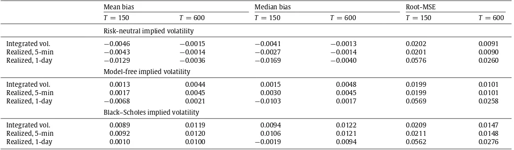
Monte Carlo simulation results. The table reports the estimation results for the volatility risk premium parameter,λ, based on 500 replications. The benchmark parameter values areκ=0.10,θ=0.20,σ=0.10,λ= −0.20, andρ= −0.50 respectively.
Mean bias Median bias Root-MSE
T=150 T=600 T=150 T=600 T=150 T=600 Risk-neutral implied volatility
Integrated vol. −0.0046 −0.0015 −0.0041 −0.0013 0.0202 0.0091 Realized, 5-min −0.0043 −0.0014 −0.0027 −0.0014 0.0201 0.0090 Realized, 1-day −0.0129 −0.0036 −0.0169 −0.0040 0.0576 0.0260
Model-free implied volatility
Integrated vol. 0.0013 0.0044 0.0015 0.0048 0.0199 0.0101
Realized, 5-min 0.0017 0.0045 0.0030 0.0045 0.0199 0.0101
Realized, 1-day −0.0068 0.0021 −0.0103 0.0017 0.0569 0.0258 Black–Scholes implied volatility
Integrated vol. 0.0089 0.0119 0.0094 0.0122 0.0209 0.0147
Realized, 5-min 0.0092 0.0120 0.0106 0.0121 0.0211 0.0148
Realized, 1-day 0.0010 0.0100 −0.0019 0.0094 0.0562 0.0276
Table 1summarizes the parameter estimation for the volatility risk premium. The use of model-free implied volatility achieves a similar root-mean-squared error (RMSE) and convergence rate as the true infeasible risk-neutral implied volatility. On the other hand, the use of Black–Scholes implied volatilities adversely affects the estimated volatility risk premium, especially for the large
sample size (T
=
600). Also, the estimates based on realizedvolatility from five-minute returns (over a monthly horizon) has virtually the same small bias and efficiency as the estimates based on the (infeasible) integrated volatility. In contrast, the use of realized volatilities from daily returns generally results in a larger biases and noticeable lower efficiency.10
4. Estimates for the market volatility risk premium
4.1. Volatility risk premium and relative risk aversion
There is an intimate link between the stochastic volatility risk premium and the coefficient of risk aversion for the representative investor within the standard intertemporal asset pricing framework. In particular, assuming a linear volatility risk premium along with an affine version of the stochastic volatility model corresponding to
σ
t(
·
)
=
σ
√
Vtin(1), as inHeston(1993),
it follows that
−
λ
Vt=
covt
dmt
mt
,
dVt
,
(10)wheremtdenotes the pricing kernel, or marginal utility of wealth
for the representative investor. Moreover, if we assume that the representative agent has a power utility function
Ut
=
e−δtW1−γ t
1
−
γ
,
(11)where
δ
denotes a constant subjective time discount rate, and inequilibrium the agent holds the market portfolio, marginal utility equalsmt
=
e−δtW−γt . It follows then from Itô’s formula that11
covt
dmt
mt
,
dVt
= −
γ ρσ
Vt.
(12)leverage, orρ= −0.80. These additional designs as well as the estimation results for theκandθparameters are available upon request.
10 The Wald test for the risk premium parameter, as well as GMM omnibus test, also has the correct size for the model-free risk-neutral and realized volatility measures. These additional graphs are omitted to conserve space but available upon request.
11 A similar reduced-form argument is made byBakshi and Kapadia(2003). For a much earlier formal general equilibrium treatment, see alsoBates(1988) who allows for both stochastic volatility and jumps.
Combining (10) and (12), the constant relative risk aversion
coefficient
γ
is directly proportional to the volatility risk premium:γ
=
λ/(ρσ )
. Moreover, given the estimated values ofρ
=
−
0.
8 andσ
=
1.
2 for the S&P500 data analyzed below,−
λ
is approximately equal to the representative investor’s risk aversion,γ
. An argument along the lines ofGordon and St-Amour(2004)suggests that the above line of reasoning relating the volatility risk premium to investor risk aversion still applies in an approximate
sense if investor risk aversion
γ
t is time-varying and follows adiffusion process.12
4.2. Empirical approximation for the volatility risk premium
The discussion in the previous section shows how our approach can accommodate a time-varying volatility risk premium. Previ-ous efforts to explain time-varying volatility risk premia with eco-nomic variables have been rare and challenging at best. In contrast, the model and GMM estimation procedure that we use here are quite simple to implement.
Specifically, we approximate the volatility risk premium parameter as following an augmented AR(1) process,
λ
t+1=
a+
bλ
t+
K−
k=1
ck
×
statet,k,
(13)where ‘‘statet,k’’ are macro-finance state variables. To be consistent
with an absence of arbitrage, the macro-finance shocks ‘‘statet,k’’
must be interpreted either as fixed covariates or predetermined functions of the time-tstate variables,StandVt. We estimate this
time-varying risk premium specification by adding lagged squared realized volatility, lagged implied volatility, and six out of the seven macro-finance covariates (without the redundant lagged realized
volatility, see Section4.5 for details) as additional instruments
for the cross moment in(8), leaving the moment for the realized
volatility in(5)the same as in the constant risk premium case. All-in-all, this results in the sameX2
(
1)
asymptotic distribution forthe GMM omnibus test as in the estimation with a constant
λ
.4.3. Data sources and summary statistics
Our empirical analysis is based on monthly implied and realized volatilities for the S&P500 index from January 1990 through May 2004. For the risk-neutral implied volatility measure, we rely on the VIX index provided by the Chicago Board of Options
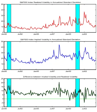
Fig. 1. Model-free realized and implied volatilities.
Exchange (CBOE). The VIX index, available back to January 1990, is based on the liquid S&P500 index options, and more importantly, it is calculated based on the model-free approach discussed
earlier.13Under appropriate assumptions, the concept of CBOE’s
‘‘fair value of future variance’’ developed byDemeterfi et al.(1999) is identical to the ‘‘model-free implied variance’’ byBritten-Jones and Neuberger(2000), as well as the ‘‘risk-neutral expected value of the return variance’’ byCarr and Wu(2009) (seeJiang and Tian, 2007, for detailed justification). As shown in the Monte Carlo study, the model-free implied volatility should be a good approximation to the true (unobserved) risk-neutral expectation of the integrated volatility.
Our realized volatilities are based on the summation of the five-minute squared returns on the S&P500 index within the
month.14Thus, for a typical month with 22 trading days, we have
22
×
78=
1716 five-minute returns, where the 78 five-minutesubintervals cover the normal trading hours from 9:30 am to 4:00 pm, including the close-to-open five-minute interval. Again, as indicated by the Monte Carlo simulations discussed in the
13 In September 2003, CBOE replaced the old VIX index, based on S&P100 options and Black–Scholes implied volatility, with the new VIX index based on S&P500 options and model-free implied volatilities involving a discrete approximation to the theoretical result inCarr and Madan(1998). Historical data on both the old and new VIX are directly available from the CBOE.
14 The high-frequency data for the S&P500 index is provided by the Institute of Financial Markets.
previous section, the monthly realized volatilities based on these five-minute returns should provide a very good approximation to the true (unobserved) continuous-time integrated volatility, and, in particular, a much better approximation than the one based on the sum of the daily squared returns.
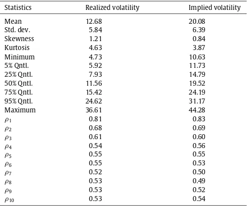
Fig. 1 plots realized volatility, implied volatility, and their difference.15Both of the volatility measures were generally higher during the latter half of the sample, although they have also both decreased more recently. Summary statistics are reported in
Table 2. Realized volatility is systematically lower than implied volatility, and its unconditional distribution deviates more from the normal. Both measures exhibit pronounced serial correlation with extremely slow decay in their autocorrelations.
The difference between the implied and realized volatilities is sometimes used by market participants as a measure for the
market-implied risk aversion.16 However, the raw difference,
depicted in the bottom panel inFig. 1, is obviously rather noisy
and more or less reflects the overall level of the volatility. A more structured approach for extracting the volatility risk premium (or implied risk aversion), as discussed in the previous sections, thus holds the promise of revealing a better picture and a deeper
15 Here and throughout the paper, monthly standard deviations are ‘‘annualized’’ by multiplying by√12.
Table 2
Summary statistics for monthly volatilities.
Statistics Realized volatility Implied volatility
Mean 12.68 20.08
Std. dev. 5.84 6.39
Skewness 1.21 0.84
Kurtosis 4.63 3.87
Minimum 4.73 10.63
5% Qntl. 5.92 11.73
25% Qntl. 7.93 14.79
50% Qntl. 11.56 19.52
75% Qntl. 15.42 24.19
95% Qntl. 24.62 31.17
Maximum 36.61 44.28
ρ1 0.81 0.83
ρ2 0.68 0.69
ρ3 0.61 0.60
ρ4 0.54 0.56
ρ5 0.55 0.55
ρ6 0.55 0.53
ρ7 0.52 0.50
ρ8 0.53 0.49
ρ9 0.53 0.52
ρ10 0.53 0.54
understanding of the way in which the volatility risk premium evolves over time, and its relationship to the macroeconomy. We next turn to a discussion of our pertinent estimation results.
4.4. Preliminary factor analysis and modeling assumptions
Our analysis relies on the stochastic volatility model(1)and
its corresponding risk-neutral counterpart(2). While our approach is quite general in that the functions
µ
t(
·
)
andσ
t(
·
)
can be leftunspecified, there are some assumptions embedded in Eqs.(1)–(2)
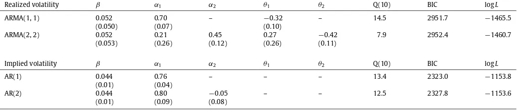
that can be tested before going further: realized volatility should follow an ARMA(1, 1) process; model-free implied volatility should follow an AR(1) process; and one common factor drives both integrated and implied volatility.
To test whether realized volatility and model-free implied volatility follow ARMA(1, 1) and AR(1) processes, respectively, we compare the ARMA(1, 1) with an ARMA(2, 2) model and the AR(1) with an AR(2) model. The results are reported inTable 3. All four models produce white-noise residuals (the portmanteau tests do not reject the hypothesis of white-noise residuals at conventional levels). Meanwhile, following a traditional time-series approach to model selection based on the minimization of Schwartz’s Bayesian information criterion, the ARMA(1, 1) is preferred to the ARMA(2, 2) for realized volatility and the AR(1) is preferred to the AR(2) for model-free implied volatility.17
The third model implication listed above holds that realized and model-free implied volatility are driven by a single common factor. To informally investigate this, we performed a standard (unconditional) principal components analysis (PCA) on the two volatility series. The PCA indicates that the first principal component explains 79% of the variance of the two series. This is high enough to assure us that our (implicit) assumption of a single common factor is not obviously violated by the data. Of course, the remaining 21% of the variability could be explained, at least in part, by a time-varying volatility risk premium.
We next turn our attention to the results from the more formal GMM-based estimation strategy.
17 While a standard likelihood ratio (LR) test based on the reported maximized values for the Gaussian log likelihoods results in the ARMA(1, 1) for the realized volatility being rejected in favor of the ARMA(2, 2) model, the errors from both models (the volatility-of-volatility) are heteroskedastic, so the standard critical values likely overstates the difference in fit between the two models.
[image:6.595.34.284.83.291.2]4.5. GMM estimation results
Table 4reports the GMM estimation results for two volatility risk premium specifications: (i) a constant
λ
; (ii) a time-varyingλ
tdriven by shocks to macro-finance variables as in Eq.(13).18 As seen in the first column of the table, when we restrict
the risk premium to be constant, the estimated
λ
is negativeand statistically significant. This finding is consistent with other papers that have found a negative risk premium on stochastic volatility. However, the chi-square omnibus test of overidentifying restrictions rejects the overall specification at the 10% (although not at the 5%) level.
The second column presents the results obtained by explicitly including macro-finance covariates. To select the macro-finance variables in the time-varying risk premium specification, we did
an extensive search over 29 monthly data series.19 If part of
the temporal variation in investor risk aversion reflects investors focusing on different aspects of the economy at different points in time, as seems likely, some flexibility in specifying the set of covariates seems both appropriate and unavoidable. Hence, we select the group of variables that jointly achieves the highest
p-value of the GMM omnibus specification test and that are
significant (at the 5% level) based on their individual t-test
statistics. To facilitate the subsequent discussion, the resulting seven variables have all been standardized to have mean zero and variance one so that their marginal contribution to the
time-varying risk premium are directly comparable.20
The results for the autoregressive part of the specification
implies an average risk premium ofa
/(
1−
b)
= −
1.
82, and,without figuring in the dynamic impact of the macro state
variables, an even higher degree of own persistence,b
=
0.
93.As necessitated by the specification search, all of the individual parameters for the macro-finance covariates are statistically significant at the 5% level, and the overall GMM specification test is greatly improved, with ap-value of 0.68. The resulting estimate for the volatility risk premium is plotted in the top panel ofFig. 2.
Both the signs and magnitudes of the macro-finance shock coefficients are important in understanding the time-variation of the volatility risk premium. Sticking to the convention that (
−
λ
) represents the risk premium, or risk aversion, the realized volatility has the biggest contribution (−
0.32) and a positive impact (i.e., when volatility is high so is risk aversion). The impact of AAA bond spread over Treasuries (0.19) likely reflects a business cycle effect (i.e., credit spreads tend to be high before a downturn which usually coincides with low risk aversion). Conversely, housingstarts have a positive impact on the risk premium (
−
0.19) (i.e.,a real estate boom usually precedes higher risk aversion). The P
/
Eratio is the fourth most important factor (0.14), and impactsthe premium negatively (i.e., everything else equal, higherP
/
Eratios lowers the degree of risk aversion). The fifth variable in the table is industrial production growth (0.10), which also has a negative impact (i.e., higher growth leads to a lower volatility risk premium). On the contrary, the sixth PPI inflation variable leads to higher risk aversion (
−
0.05). Finally, the last significant macro state variable, payroll employment, marginally raises the volatility risk premium (−
0.04), possibly as a result of wage pressure.18 In order to conserve space, we only report the results pertaining to the parameters for the volatility risk premium. The results for the other parameters in the model are directly in line with previous results reported in the literature, and consistent with the summary statistics inTable 2, point toward a high degree of volatility persistence in the (latent)Vtprocess.
19 The list of these macro-finance variables is omitted to conserve space but available upon request.
Table 3
Alternatives model specifications. For realized volatility, we estimate the ARMA(2, 2) model
Vt+∆,t+2∆=β+α1Vt,t+∆+α2Vt−∆,t+et+∆,t+2∆+θ1et,t+∆+θ2et−∆,t
where the ARMA(1, 1) model restrictsα2=θ2=0. For implied volatility, we estimate the AR(2) model
IV∗
t+∆,t+2∆=β+α1IV∗t,t+∆+α2IV∗t−∆,t+et+∆,t+2∆
where the AR(1) model restrictsα2=0. Standard errors are shown in parentheses. The columns labeled ‘‘Q(10)’’, ‘‘BIC’’ and ‘‘logL’’ show the Ljung–Box portmanteau test statistic for white-noise residuals using ten lags, Schwartz’s Bayesian information criterion, and the maximized value of the Gaussian log-likelihood, respectively.
Realized volatility β α1 α2 θ1 θ2 Q(10) BIC logL
ARMA(1, 1) 0.052 0.70 – −0.32 – 14.5 2951.7 −1465.5
(0.050) (0.07) (0.10)
ARMA(2, 2) 0.052 0.21 0.45 0.27 −0.42 7.9 2952.4 −1460.7
(0.053) (0.26) (0.12) (0.26) (0.11)
Implied volatility β α1 α2 θ1 θ2 Q(10) BIC logL
AR(1) 0.044 0.76 – – – 13.4 2323.0 −1153.8
(0.01) (0.04)
AR(2) 0.044 0.80 −0.05 – – 12.5 2327.8 −1153.6
(0.01) (0.09) (0.08)
Table 4
Estimation of volatility risk premium. All of the macro-finance variables are standardized to have mean zero and variance one. The growth variables (Industrial Production, Producer Price Index, and Payroll Employment) are expressed in terms of the logarithmic difference over the past twelve months. The lag length in the Newey–West weighting matrix employed in the estimation, as discussed in the main text, is set at 25.
Constant Macro-finance
λ −1.793 (0.216)
a −0.122 (0.051)
b 0.933 (0.030)
c1Realized volatility −0.319 (0.042)
c2Moody AAA bond spread 0.194 (0.034)
c3Housing start −0.191 (0.055)
c4S&P500P/Eratio 0.140 (0.015)
c5Industrial production 0.097 (0.026)
c6Producer price index −0.047 (0.023)
c7Payroll employment −0.040 (0.019)
X2(d.o.f.=1)(p-value) 2.889 (0.089) 0.169 (0.681)
4.6. Robustness checks
The consistency of the realized volatility estimator hinges on the idea of ever finer sampled observations over a fixed-length time interval. Yet, it is well-known that a host of market microstructure frictions, including price discreteness and staleness, invalidate the basic underlying martingale assumption
at the ultra high frequencies.21 In order to investigate the
robustness of our findings based on the 5-min returns with respect to this issue, we re-estimate our model with realized volatilities constructed from coarser sampled 30-min returns. As seen from the first column inTable 5, the sign and significance of the parameter estimates are qualitatively and quantitatively very similar to the previous findings, and thep-values for the overall goodness-of-fit tests for the model are also remarkably close (0.697 versus 0.681).
The Monte Carlo experiment in Section3 indicates that the
use of Black–Scholes as opposed to model-free implied volatilities does not result in materially different estimates for the (constant) volatility risk premium, when the sample size is relatively small (150 months). To investigate the sensitivity of our results to the
21 A large, and rapidly growing, literature have sought different ways in which to best deal with these complications in the construction of improved realized volatility measures; see, e.g.,Aït-Sahalia et al. (2005);Bandi and Russell (2006); Hansen and Lunde (2006).
specific volatility measure, the second column inTable 5reports
the GMM estimation results obtained by using Black–Scholes implied volatilities in place of the model-free measures. Compared to the original results in the last column inTable 4, the parameter estimates are generally close, as are their standard errors. This is in line with the Monte Carlo evidence presented earlier, which indicates that the inferior performance of Black–Scholes becomes more apparent for larger sample sizes (600 months).
It is been widely argued in the literature that most major market indices contain jumps, or price discontinuities (see, e.g., Bates,
1996; Bakshi et al., 1997; Pan, 2002; Chernov et al., 2003). This suggests that it may be important to separately consider jump risk when estimating the stochastic volatility risk premium.
However, the moment condition in Eq.(8)only identifies a single
risk premium parameter. Thus, to check the robustness of our estimates with respect to jumps, we simply fix the jump risk premium and re-estimate the resulting volatility risk premium.
To identify the jumps, we followBarndorff-Nielsen and Shephard
(2006, 2004c) in using the difference between the realized
volatility,
Vtn,t+∆
≡
n
−
i=1
pt+i
n(∆)
−
pt+i−n1(∆)
2→
∫
t+∆t
Vsds
+
∫
t+∆t
Js2ds
,
(14)and the so-called bi-power variation,
BVnt,t+∆
≡
n
−
i=2
pt+i
n(∆)
−
pt+ i−1n (∆)
pt+i−1
n (∆)
−
pt+ i−2n (∆)
→
∫
t+∆t
Vsds
,
(15)for measuring the monthly jump volatility,
t+∆t J
2
sds, under the
objective measure (see alsoHuang and Tauchen, 2005;Andersen
et al., 2007). Following Jiang and Tian (2005) and Carr and
Wu (2009) the model-free implied volatility may be similarly
decomposed under the risk-neutral expectation,
IV∗
t,t+∆
≈
E∗∫
t+∆t
Vsds
Ft
+
E∗∫
t+∆t
Js2ds
Ft
.
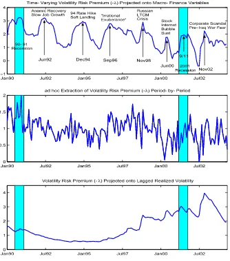
(16) [image:7.595.46.294.335.457.2]Fig. 2. Estimates of time-varying volatility risk premia.
Table 5
Robustness checks. All of the macro-finance variables are the same as in the previous table. 30-min refers to the use of realized volatilities based on 30-min returns. BSIV replaces the model-free implied volatility with Black–Scholes implied volatility. Jump (1), (2), and (3) represent the cases where the risk-neutral expectation of squared jumps is assumed to be the same, double, and tipple that of the objective expectation.
Macro-finance specification 30-min BSIV Jump (1) Jump (2) Jump (3)
a −0.156 (0.040) −0.129 (0.065) −0.158 (0.055) −0.145 (0.048) −0.129 (0.050)
b 0.891 (0.028) 0.933 (0.033) 0.916 (0.032) 0.919 (0.029) 0.925 (0.030)
c1Realized volatility −0.262 (0.102) −0.281 (0.033) −0.352 (0.049) −0.365 (0.063) −0.386 (0.070)
c2Moody AAA bond spread 0.107 (0.065) 0.151 (0.029) 0.225 (0.039) 0.229 (0.054) 0.236 (0.056)
c3Housing start −0.175 (0.054) −0.142 (0.056) −0.199 (0.056) −0.203 (0.056) −0.209 (0.057)
c4S&P500P/Eratio 0.136 (0.021) 0.129 (0.014) 0.144 (0.013) 0.147 (0.012) 0.152 (0.011)
c5Industrial production 0.064 (0.054) 0.056 (0.026) 0.110 (0.028) 0.117 (0.032) 0.124 (0.033)
c6Producer price index −0.037 (0.019) −0.032 (0.021) −0.048 (0.024) −0.046 (0.022) −0.043 (0.021)
c7Payroll employment −0.019 (0.043) −0.013 (0.020) −0.045 (0.020) −0.051 (0.023) −0.059 (0.024) X2(d.o.f.=1)(p-value) 0.151 (0.697) 0.373 (0.541) 0.150 (0.698) 0.059 (0.807) 0.004 (0.951)
the jump contribution differ by a constant multiple. In particular, under Jump Scenario (h),
E∗
∫
t+∆ tJs2ds
Ft
=
h·
E∫
t+∆t
Js2ds
Ft
.
(17)The corresponding estimation results, reported in the last three
columns inTable 5, show that the level, persistence, and
macro-finance sensitivities of the volatility risk premium are all largely unaffected. Interestingly, on comparing the three jumps scenarios, the overall goodness-fit appears to improve as the price of jump
risk increases. Nonetheless, overall the results clearly confirm the robustness of our previous findings with respect to the specific
jump dynamics and risk prices entertained here.22
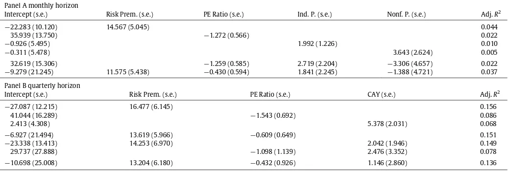
[image:8.595.36.554.512.627.2]Table 6
Stock market return predictability. Panel A reports predictive regressions for the monthly excess return on S&P500 index measured in annualized percentage term. Industrial Production (Ind. P.) and Nonfarm Payroll Employment (Nonf. P.) numbers represent the past year logarithmic changes in annualized percentages. The PE Ratio is based on the trailing twelve month earning reported for S&P500 index. Risk Prem. refers to the volatility risk premium extracted here. Panel B reports predictive regressions for the quarterly excess return on S&P500 index from 1990Q1 to 2003Q2. The consumption-wealth-ratio, or CAY, is defined inLettau and Ludvigson(2001), and the data is downloaded from their website.
Panel A monthly horizon
Intercept (s.e.) Risk Prem. (s.e.) PE Ratio (s.e.) Ind. P. (s.e.) Nonf. P. (s.e.) Adj.R2
−22.283 (10.120) 14.567 (5.045) 0.044
35.939 (13.750) −1.272 (0.566) 0.022
−0.926 (5.495) 1.992 (1.226) 0.010
−0.311 (5.478) 3.643 (2.624) 0.005
32.619 (15.306) −1.259 (0.585) 2.719 (2.204) −3.306 (4.657) 0.022 −9.279 (21.245) 11.575 (5.438) −0.430 (0.594) 1.841 (2.245) −1.388 (4.721) 0.037 Panel B quarterly horizon
Intercept (s.e.) Risk Prem. (s.e.) PE Ratio (s.e.) CAY (s.e.) Adj.R2
−27.087 (12.215) 16.477 (6.145) 0.156
41.044 (16.289) −1.543 (0.692) 0.086
2.413 (4.308) 5.378 (2.031) 0.068
−6.927 (21.494) 13.619 (5.966) −0.609 (0.649) 0.151
−23.338 (13.413) 14.253 (6.970) 2.042 (1.946) 0.149
29.737 (27.888) −1.098 (1.139) 2.476 (3.352) 0.078
−10.698 (25.008) 13.204 (6.180) −0.432 (0.926) 1.146 (2.860) 0.136
4.7. Comparing alternative estimates of time-varying risk premia
Several alternative procedures for estimating the time-varying volatility risk premium have previously been implemented in the literature. One approach is to vary the risk premium parameter each time period to best match that period’s market data. In the context of volatility modeling, that approach would vary the risk premium parameter to match each month’s difference between realized and implied volatility (papers that have taken
this approach includeRosenberg and Engle (2002, p. 363) and
Tarashev et al. (2003, p. 62)). In the context of our modeling framework, such an approach produces the time-varying risk
premium shown in the middle panel ofFig. 2. The general shape of
Fig. 2matches the simple difference between implied and realized volatilities shown in the bottom panel ofFig. 1.
As previously noted, because this approach attributes every wiggle in the data to changes in the risk premium, it produces a very volatile time series of monthly risk premia. Economic theory argues that an asset’s risk premium should depend on deep structural parameters. For example, in the consumption CAPM (C-CAPM), an asset’s risk premium varies with investors’ risk aversion and the asset’s covariance with investors’ consumption. By definition, deep structural parameters should be relatively stable over time. Yet the approach of period-by-period estimation of a time-varying risk premia forces the parameters to vary (almost independently) from one period to the next. As such, we find that monthly volatility risk premiums estimated in this way are implausibly volatile.
A second approach to estimating risk premium parameters comes from the consumption-based asset pricing literature. This approach typically assumes that risk premia are constant, or if risk preferences are allowed to vary over time, they end up being implausibly smooth and possibly nonstationary. For example,
Campbell and Cochrane (1999) generate time variation in risk aversion through habit formation in which the level of habit reacts only gradually to changes in consumption. Such a modeling strategy explicitly prevents the risk premia from being excessively variable in the short-run. Risk aversion parameters estimated with
this approach (Brandt and Wang, 2003, p. 1481 andGordon and
St-Amour, 2004, p. 249) generally have little or no variation at a business cycle frequency.
In contrast, our estimated volatility risk premium parameter
shown in the top panel of Fig. 2, has plausible business cycle
variation. Peaks and troughs in the series are typically multiple years apart, and the series dies not have excessive month-by-month fluctuations that. The estimated risk premium rises sharply during the two NBER-dated macroeconomic recessions (the shaded areas in the plots), as well as the periods of slow recovery and job growth after the 1991 and 2001 recessions. Nearly all of the peaks in the series are readily identifiable with major macroeconomic or financial market developments, as labeled in the figure. The chart also suggests that the risk premium often rises sharply but declines only gradually.
It is interesting to contrast these estimates with the plot in the bottom panel in the same figure, which shows the estimate of the volatility risk premium based solely on the lagged realized volatility as the only state variable. The resulting risk premium hardly changes over the first half of the sample and otherwise appears extremely smooth. We conclude that the macro-finance variables clearly help in identifying a reasonably informative time-varying volatility risk premium.
4.8. Stock return predictability
Because the volatility risk premium can be related to investor risk aversion, it may be informative about other risk premia in the economy. To illustrate, we compare its predictive power for aggregate stock market returns with that of other
traditionally-used macro-finance variables. The top panel ofTable 6reports
the results of simple regressions of monthly S&P500 excess returns on the volatility risk premium and on the most significant individual variables from the pool of 29 macro-finance covariates. The extracted volatility risk premium has the highest predictive
power with an adjustedR2of 4.4%.23The second best predictor
is the P
/
Eratio with an adjusted R2 of 2.2%. Next in order areindustrial production and nonfarm payrolls with adjusted R2’s
of 1.0% and 0.5%, respectively. Dividend yield – a significant predictor according to many other studies – only explains 0.3% of the monthly return variation. These results are consistent with previous findings that macroeconomic state variables do predict
returns, though the predictability measured by adjusted R2 is
usually in the low single digits. Nonetheless, it is noteworthy that of all the predictor variables, the volatility risk premium results in the highest adjustedR2.
Combining all of the marginally significant variables into a single multiple regression together with the volatility risk premium, none of the macro-finance variables are significant, while only theP
/
Eratio is significant in the regression excluding the premium. Of course, the estimate for the volatility risk premium already incorporates some of the same macroeconomicvariables (see Table 4), so the finding that these variables are
‘‘driven out’’ when included together with the premium is not necessarily surprising. However, the macro-variables entering
the model for
λ
t only impact the returns indirectly throughthe temporal variation in the premium, and the volatility risk premium itself is also estimated from a different set of moment conditions involving only the model-free realized and option-implied volatilities.
The bottom panel ofTable 6examines stock return
predictabil-ity over a quarterly horizon. In addition to the volatilpredictabil-ity risk
premium and theP
/
Eratio from the last month of the previousquarter, which were the two most important predictor variables in the monthly regressions, we add the quarterly consumption-wealth ratio. The consumption-consumption-wealth ratio, termed CAY, has pre-viously been found byLettau and Ludvigson(2001) to be helpful in explaining longer-horizon returns.
The first three regressions in the bottom panel ofTable 6show
that each of the three predictor variables are statistically significant in univariate regressions. The volatility risk premium results in the highest individual adjustedR2of 15.6%. Adding theP
/
Eratio or CAY to the volatility risk premium results in lower adjustedR2’s and only the risk premium remains statistically significant in all of the predictive regressions.245. Conclusion
This paper develops a simple consistent approach for estimating the volatility risk premium. The approach exploits the linkage between the objective and risk-neutral expectations of the integrated volatility. The estimation is facilitated by the use of newly available model-free realized volatilities based on high-frequency intraday data along with model-free option-implied volatilities. The approach allows us to explicitly link any temporal variation in the risk premium to underlying state variables within an internally consistent and simple-to-implement GMM estimation framework. A small-scale Monte Carlo experiment indicates that the procedure performs well in estimating the volatility risk premium in empirically realistic situations. In contrast, the estimates based on Black–Scholes implied volatilities and/or monthly sample variances based on daily squared returns result in inefficient and statistically less reliable estimates of the risk premium. Applying the methodology to the S&P500 market index, we find significant evidence for temporal variation in the volatility risk premium, which we directly link to a set of underlying macro-finance state variables. Interestingly, the extracted volatility risk premium also appears to be helpful in predicting the return on the market itself.
The volatility risk premium (or risk aversion index) extracted in our paper differs sharply from other approaches in the
24 The predictability of the volatility risk premium documented here, 4.4% and 15.6% at the monthly and quarterly horizons, respectively, far exceed that afforded by other more traditional predictor variables. Of course, by estimating the volatility premium from the entire sample, the results suffer from a look-ahead bias. Also, with only 173 monthly and 54 quarterly return observations, the specific estimates may be driven by a few influential outliers. Still, the more comprehensive empirical investigation reported inBollerslev et al.(2008) do suggest that the results hold up more generally, although the magnitude of the reportedR2’s probably overstate the case.
literature. In particular, earlier estimates relying on period-by-period differences in the estimated risk-neutral and objective distributions tend to produce implausibly volatile estimates. On the other hand, earlier procedures based on structural macroeconomic/consumption-type pricing models typically result in implausibly smooth estimates. In contrast, the model-free realized and implied volatility-based procedure developed here results in an estimated premium that avoids the excessive period-by-period random fluctuations, yet responds to recessions, financial crises, and other economic events in an empirically realistic fashion.
It would be interesting to more closely compare and contrast the risk aversion index estimated here to other popular gauges of investor fear or market sentiment. Also, how does the estimated volatility risk premium for the S&P500 compare to that of other markets? The results in the paper show that the extracted volatility risk premium for the current month is useful in predicting next month’s aggregate S&P500 return. It would be interesting to further explore the cross sectional pricing implications of this finding. Does the volatility risk premium represent a systematic
priced risk factor?25 Also, what is the link between stock and
bond market volatility risk premia? Lastly, better estimates for the volatility risk premium are, of course, of direct importance for derivatives pricing. We leave further work along these lines for future research.
References
Adrian, Tobias, Rosenberg, Joshua, 2008. Stock returns and volatility: pricing the long-run and short-run components of market risk. Journal of Finance 63, 2997–3030.
Aït-Sahalia, Yacine, Kimmel, Bob, 2007. Maximum likelihood estimation of stochastic volatility models. Journal of Financial Economics 83, 413–452. Aït-Sahalia, Yacine, Lo, Andrew W., 2000. Nonparametric risk management and
implied risk aversion. Journal of Econometrics 94, 9–51.
Aït-Sahalia, Yacine, Mykland, Per, Zhang, Lan, 2005. How often to sample a continuous-time process in the presence of market microstructure noise. Review of Financial Studies 18, 351–416.
Amihud, Yakov, Hurvich, Clifford, 2004. Predictive regressions: a reduced-bias estimation method. Journal of Financial and Quantitative Analysis 39, 813–841. Andersen, Torben G., Bollerslev, Tim, Diebold, Francis X., 2007. Roughing it up: including jump components in the measurement, modeling, and forecasting of return volatility. Review of Economics and Statistics 89, 701–720.
Andersen, Torben G., Bollerslev, Tim, Diebold, Francis X., 2009. Parametric and Nonparametric Volatility Measurement. In: Handbook of Financial Econometrics. Elsevier Science B.V., Amsterdam (Chapter 2) (forthcoming). Andersen, Torben G., Bollerslev, Tim, Diebold, Francis X., Ebens, Heiko, 2001. The
distribution of realized stock return volatility. Journal of Financial Economics 61, 43–76.
Andersen, Torben G., Bollerslev, Tim, Diebold, Francis X., Labys, Paul, 2003. Modeling and forecasting realized volatility. Econometrica 71, 579–625.
Andersen, Torben G., Bollerslev, Tim, Meddahi, Nour, 2004. Analytical evaluation of volatility forecasts. International Economic Review 45, 1079–1110.
Ang, Andrew, Hodrick, Robert, Xing, Yuhang, Zhang, Xiaoyan, 2006. The cross-section of volatility and expected returns. Journal of Finance 61, 259–299. Bakshi, Gurdip, Cao, Charles, Chen, Zhiwu, 1997. Empirical performance of
alternative option pricing models. Journal of Finance 52, 2003–2049. Bakshi, Gurdip, Kapadia, Nikunj, 2003. Delta-hedged gains and the negative market
volatility risk premium. Review of Financial Studies 16, 527–566.
Bandi, Federico, Russell, Jeffrey, 2006. Separating microstructure noise from volatility. Journal of Financial Economics 79, 655–692.
Barndorff-Nielsen, Ole, Shephard, Neil, 2002. Econometric analysis of realised volatility and its use in estimating stochastic volatility models. Journal of the Royal Statistical Society, Series B 64.
Barndorff-Nielsen, Ole, Shephard, Neil, 2004a. Econometric analysis of realised covariation: high frequency based covariance, regression and correlation. Econometrica 72, 885–925.
Barndorff-Nielsen, Ole, Shephard, Neil, 2004b. A feasible central limit theory for realised volatility under leverage. Manuscript. Nuffield College, Oxford University.
Barndorff-Nielsen, Ole, Shephard, Neil, 2004c. Power and bipower variation with stochastic volatility and jumps. Journal of Financial Econometrics 2, 1–48.
Barndorff-Nielsen, Ole, Shephard, Neil, 2006. Econometrics of testing for jumps in financial economics using bipower variation. Journal of Financial Econometrics 4, 1–30.
Bates, David S., 1988. Pricing options on jump-diffusion process. Working Paper. Rodney L. White Center, Wharton School.
Bates, David S., 1996. Jumps and stochastic volatility: exchange rate process implicit in deutsche mark options. The Review of Financial Studies 9, 69–107. Bekaert, Geert, Engstrom, Eric, Grenadier, Steven R., 2005. Stock and bond returns
with moody investors. Working Paper. Columbia University.
Bekaert, Geert, Engstrom, Eric, Xing, Yuhang, 2009. Risk, uncertainty and asset prices. Journal of Financial Economics 91, 39–82.
Benzoni, Luca, 2002. Pricing options under stochastic volatility: an empirical investigation. Working Paper. University of Minnesota.
Bliss, Robert R., Panigirtzoglou, Nikolaos, 2004. Option-implied risk aversion estimates. Journal of Finance 59, 407–446.
Bollerslev, Tim, Tauchen, George, Zhou, Hao, 2008. Variance risk premia and expected stock returns. Working Paper. Department of Economics, Duke University.
Bollerslev, Tim, Zhou, Hao, 2002. Estimating stochastic volatility diffusion using conditional moments of integrated volatility. Journal of Econometrics 109, 33–65.
Bollerslev, Tim, Zhou, Hao, 2006. Volatility puzzles: a simple framework for gauging return-volatility regressions. Journal of Econometrics 131, 123–150. Brandt, Michael W., Wang, Kevin Q., 2003. Time-varying risk aversion and expected
inflation. Journal of Monetary Economics 50, 1457–1498.
Britten-Jones, Mark, Neuberger, Anthony, 2000. Option prices, implied price processes, and stochastic volatility. Journal of Finance 55, 839–866.
Campbell, John Y., 1987. Stock returns and the term structure. Journal of Financial Economics 18, 373–399.
Campbell, John Y., Cochrane, John H., 1999. By force of habit: a consumption based explanation of aggregate stock market behavior. Journal of Political Economy 107, 205–251.
Campbell, John Y., Shiller, Robert J., 1988a. The dividend-price ratio and expectations of future dividends and discount factors. Review of Financial Studies 1, 195–228.
Campbell, John Y., Shiller, Robert J., 1988b. Stock prices, earnings, and expected dividends. Journal of Finance 43, 661–676.
Carr, Peter, Madan, Dilip, 1998. Towards a Theory of Volatility Trading. Risk Books, pp. 417–427 (Chapter 29).
Carr, Peter, Wu, Liuren, 2009. Variance risk premiums. Review of Financial Studies 22, 1311–1341.
CBOE Documentation 2003. VIX: CBOE volatility index. White Paper.
Chernov, Mikhail, Gallant, A. Ronald, Ghysels, Eric, Tauchen, George, 2003. Alternative models for stock price dynamics. Journal of Econometrics 116, 225–257.
Chernov, Mikhail, Ghysels, Eric, 2000. A study towards a unified approach to the joint estimation of objective and risk neutral measures for the purpose of options valuation. Journal of Financial Economics 56, 407–458.
Cochrane, John H., Piazzesi, Monika, 2005. Bond risk premia. American Economic Review 95, 138–160.
Demeterfi, Kresimir, Derman, Emanuel, Kamal, Michael, Zou, Joseph, 1999. A guide to volatility and variance swaps. Journal of Derivatives 6, 9–32.
Eraker, Bjørn, 2004. Do stock prices and volatility jump? Reconciling evidence from spot and option prices. Journal of Finance 59, 1367–1403.
Fama, Eugene F., Bliss, Robert R., 1987. The information in long-maturity forward rates. The American Economic Review 77, 680–692.
Fama, Eugene F., French, Kenneth R., 1988. Dividend yields and expected stock returns. Journal of Financial Economics 22, 3–25.
Garcia, René, Lewis, Marc-André, Renault, Éric, 2010. Estimation of objective and risk-neutral distributions based on moments of integrated volatility. Journal of Econometrics, forthcoming (doi:10.1016/j.jeconom.2010.03.011).
Gordon, Stephen, St-Amour, Pascal, 2004. Asset returns and state-dependent risk preferences. Journal of Business and Economic Statistics 22, 241–252. Hansen, Lars Peter, 1982. Large sample properties of generalized method of
moments estimators. Econometrica 50, 1029–1054.
Hansen, Peter Reinhard, Lunde, Asger, 2006. Realized variance and market microstructure noise. Journal of Business and Economic Statistics 24, 127–218.
Heston, Steven, 1993. A closed-form solution for options with stochastic volatility with applications to bond and currency options. Review of Financial Studies 6, 327–343.
Huang, Xin, Tauchen, George, 2005. The relative contribution of jumps to total price variance. Journal of Financial Econometrics 3, 456–499.
Jackwerth, Jens Carsten, 2000. Recovering risk aversion from option prices and realized returns. Review of Financial Studies 13, 433–451.
Jiang, George, Oomen, Roel, 2008. Testing for jumps when asset prices are observed with noise a ‘‘swap variance’’ approach. Journal of Econometrics 144, 352–370. Jiang, George, Tian, Yisong, 2005. Model-free implied volatility and its information
content. Review of Financial Studies 1305–1342.
Jiang, George, Tian, Yisong, 2007. Extracting model-free volatility from option prices: an examination of the VIX index. Journal of Derivatives 14, 1–26. Jones, Christopher S., 2003. The dynamics of stochastic volatility: evidence from
underlying and options markets. Journal of Econometrics 116, 181–224. Lettau, Martin, Ludvigson, Sydney, 2001. Consumption, aggregate wealth, and
expected stock returns. Journal of Finance 56, 815–849.
Lynch, Damien, Panigirtzoglou, Nikolaos, 2003. Option implied and realized measures of variance. Working Paper. Monetary Instruments and Markets Division, Bank of England.
Meddahi, Nour, 2002. Theoretical comparison between integrated and realized volatility. Journal of Applied Econometrics 17, 479–508.
Newey, Whitney K., West, Kenneth D., 1987. A simple positive semi-definite, het-eroskedasticity and autocorrelation consistent covariance matrix. Economet-rica 55, 703–708.
Pan, Jun, 2002. The jump-risk premia implicit in options: evidence from an integrated time-series study. Journal of Financial Economics 63, 3–50. Rosenberg, Joshua V., Engle, Robert F., 2002. Empirical pricing kernels. Journal of
Financial Economics 64, 341–372.
Stambaugh, Robert F., 1999. Predictive regressions. Journal of Financial Economics 54, 375–421.
Tarashev, Nikola, Tsatsaronis, Kostas, Karampatos, Dimitrios, 2003. Investors’ attitude toward risk: what can we learn from options? BIS Quarterly Review. Bank of International Settlement.