arXiv:1709.06068v3 [math.MG] 28 Sep 2017
Five-dimensional Perfect Simplices
Mikhail Nevskii
∗Alexey Ukhalov
†September 18, 2017
Abstract
LetQn = [0,1]n be the unit cube in Rn,n∈N. For a nondegener-ate simplexS ⊂Rn, consider the valueξ(S) = min{σ >0 :Qn⊂σS}.
HereσSis a homothetic image ofS with homothety center at the cen-ter of gravity of S and coefficient of homothety σ. Let us introduce the value ξn = min{ξ(S) : S ⊂ Qn}. We call S a perfect simplex if
S ⊂ Qn and Qn is inscribed into the simplex ξnS. It is known that such simplices exist for n = 1 and n = 3. The exact values of ξn are known forn= 2and in the case when there exist an Hadamard matrix of order n+ 1; in the latter situation ξn =n. In this paper we show that ξ5 = 5and ξ9 = 9. We also describe infinite families of simplices S ⊂ Qn such that ξ(S) = ξn for n = 5,7,9. The main result of the paper is the existence of perfect simplices in R5.
Keywords: simplex, cube, homothety, axial diameter, Hadamard matrix
1
Introduction
Let us introduce the basic definitions. We always assume that n ∈ N. Element x∈Rn we present in component form as x = (x1, . . . , xn). Denote
Qn := [0,1]n, Q′n := [−1,1]n.
For a convex body C ⊂ Rn, by σC we mean the result of homothety of C with center of homothety at the center of gravity of C and coefficient σ.
If C is a convex polyhedron, then ver(C) means the set of vertices of C. We say that n-dimensional simplex S is circumscribed around a convex
∗Department of Mathematics, P.G. Demidov Yaroslavl State University, Sovetskaya
str., 14, Yaroslavl, 150003, Russia orcid.org/0000-0002-6392-7618 [email protected]
†Department of Mathematics, P.G. Demidov Yaroslavl State University, Sovetskaya
body C if C ⊂S and each(n−1)-dimensional face of S contains a point of C. Convex polyhedron is inscribed into C if each vertex of this polyhedron belongs to the boundary of C.
For a convex body C ⊂ Rn, by di(C) we denote the length of a longest segment in C parallel to the ith coordinate axis. The value di(C) we call
the ith axial diameter of C. The notion of axial diameter was introduced by
P. Scott in [11], [12].
For nondegenerate simplex S and convex body C inRn, we consider the value
ξ(C;S) := min{σ≥1 :C ⊂σS}.
Denote ξ(S) := ξ(Qn;S). The equality ξ(C;S) = 1 is equivalent to the inclusion C ⊂ S. For convex bodies C1, C2 ⊂ Rn, we define α(C1;C2) as
the minimal σ > 0 such that C1 belongs to a translate of σC2. Denote
α(C) := α(Qn;C). In this paper we compute the values ξ(S) and α(S) for simplices S ⊂Qn. We also consider the value
ξn := min{ξ(S) : S — n-dimensional simplex,S ⊂Qn, vol(S)6= 0}.
Let us introduce basic Lagrange polynomials of n-dimensional simplex. Let Π1(Rn) be the set of polynomials in n real variables of degree ≤ 1.
Consider a nondegenerate simplex S in Rn. Denote vertices of S by x(j) =
x(1j), . . . , x(nj)
, 1≤j ≤n+ 1,and build the matrix
A:=
x(1)1 . . . x(1)n 1 x(2)1 . . . x(2)n 1 ... ... ... ... x(1n+1) . . . x(nn+1) 1
.
Let ∆ := det(A), then vol(S) = |∆n!|. Denote by ∆j(x) the determinant
obtained from∆by changing the jth row with the row(x1, . . . , xn,1). Poly-nomials λj(x) :=
∆j(x)
∆ fromΠ1(R
n) have the propertyλ j x(k)
=δk
j, where δk
j is the Kronecker delta. Coefficients of λj form the jth column ofA−1. In the following we write A−1 = (lij), i. e., λj(x) =l1jx1+. . .+lnjxn+ln+1,j.
Each polynomial p∈Π1(Rn) can be represented in the form
p(x) =
n+1
X
j=1
p x(j)
λj(x).
x1, . . . , xn,1, we obtain n+1
X
j=1
λj(x)x(j) =x, n+1
X
j=1
λj(x) = 1. (1)
Therefore, the numbers λj(x) are barycentric coordinates of x ∈ Rn with respect to S. Simplex S can be determined by each of the systems of in-equalities λj(x)≥0 or0≤λj(x)≤1.
It is proved in [1] that forith axial diameter of simplex S holds
1
di(S)
= 1
2
n+1
X
j=1
|lij|. (2)
There exist exactly one line segment in S with the length di(S) parallel to the xi-axis. The center of this segment coincides with the point
y(i) =
n+1
X
j=1
mijx(j), mij := | lij| n+1
P
k=1|
lik|
. (3)
Each(n−1)-face ofS contains at least one of the endpoints of this segment. These results were generalized to the maximum line segment in S parallel to an arbitrary vector v 6= 0. In [4] were obtained the formulae for the length and endpoints of such a segment via coordinates of vertices of S and coordinates of v.
From equality (2) and properties of lij (see [3], Chapter 1) it follows that the value di(S)−1 is equal to the sum of the positive elements of the ith row of A−1 and simultaniously is equal to the sum of the absolute values of the negative elements of this row.
Note the following formulae for introduced numerical characteristics. Let S be a nondegenerate simplex andC be a convex body in Rn. It was shown in [3] (see § 1.3) that in the case C 6⊂S we have
ξ(C;S) = (n+ 1) max
1≤k≤n+1maxx∈C(−λk(x)) + 1. (4)
The condition
max
x∈C (−λ1(x)) =. . .= maxx∈C (−λn+1(x)) (5) is equivalent to the fact that simplexξ(S)Sis circumscribed aroundC. When C is a cube in Rn, equality (4) can be written in the form
ξ(S) = (n+ 1) max
and (5) can be replaced by the condition
max
x∈ver(C)(−λ1(x)) =. . .= maxx∈ver(C)(−λn+1(x)). (7)
ForC =Qn formula (6) was proved in [1]. The statement that (7) holds if and only if ξ(S)S is circumscribed around Qn follows from the results of [1] and [10].
It was proved in [3] (see § 1.4) that, for arbitrary convex body C and nondegenerate simplex S in Rn, holds
α(C;S) =
n+1
X
j=1
max
x∈C(−λj(x)) + 1. (8)
If C =Qn, then (8) is equivalent to
α(S) =
n
X
i=1
1
di(S)
. (9)
Equality (9) was established in [10]. There are several interesting corol-laries of this result. For instance, we present here the formula for α(S) via coefficients of λj :
α(S) = 1 2
n
X
i=1
n+1
X
j=1
|lij|. (10)
From (10) and properties of lij, it follows that α(S) is equal to the sum of the positive elements of upper n rows ofA−1 and simultaneously is equal to the sum of the absolute values of the negative elements of these rows.
It is obvious that for convex body C and simplex S holds ξ(C;S) ≥
α(C;S). The equality takes place only when simplex ξ(S)S is circumscribed around C.
IfS ⊂Qn, then di(S)≤1. Applying (9) for this case we have
ξ(S)≥α(S)≥n. (11)
Consequently, ξn ≥n. By 2009, the first author obtained that
ξ1 = 1, ξ2 =
3√5
5 + 1 = 2.34. . . , ξ3 = 3, 4≤ ξ4 ≤
13
3 = 4.33. . . ,
If n >2, then
ξn ≤
n2−3
n−1. (12)
Hence, for any n, we have n ≤ ξn < n+ 1. Inequality (12) was established by calculations for the simplexS∗ with vertices(0,1, . . . ,1),(1,0, . . . ,1),. . ., (1,1, . . . ,0), (0,0, . . . ,0) (see [2], [3], § 3.2). If n > 2, then ξ(S∗) = n2
−3
n−1,
which gives (12). If n ≥ 3, then S∗ has the following property (see [7], Lemma 3.3): replacement of an arbitrary vertex of S∗ by any point of Q
n decreases the volume of the simplex. For n = 2,3,4 (and only in these cases), S∗ is a simplex of maximum volume inQn.Ifn≥2, then di(S∗) = 1,
therefore α(S∗) = n. If n = 3, then α(S∗) = ξ(S∗); for n > 3 we have
α(S∗)< ξ(S∗).
Ifn+ 1is an Hadamard number, i.e., there exist an Hadamard matrix of the order n+ 1, thenξn=n (see section 4). In this and only this case there exist a regular simplex S inscribed into Qn such that vertices of S coincide with vertices ofQn([7], Theorem 4.5). For such a simplex, we haveξ(S) =n. It follows from (11) that α(S) =n, and (9) gives di(S) = 1.
Since 2011, the first author supposed that the equalityξn=n holds only if n+ 1 is an Hadamard number. In this paper we will demonstrate that it is not so. The smallest n such that n+ 1is not an Hadamard number, while ξn =n, is equal to 5; the next number with such a property is 9. Below we study simplices S such that S ⊂Qn⊂nS, for odd n, 1≤n ≤9. Since ξ2=
2.34... >2, there no exist such a simplex in the casen = 2. For even numbers n ≥4, the problem of existence of simplices with the condition S ⊂Qn ⊂nS is unsolved. In [5] the authors proved that ξ4 ≤ 19+5
√
13
9 = 4.1141. . ., and
conjectured that ξ4 = 19+5
√
13
9 .
A nondegenerate simplexSinRnwe will calla perfect simplex with respect
to an n-dimensional cube Q if S ⊂ Q ⊂ ξnS and cube Q is inscribed into
simplex ξnS, i. e., the boundary of ξnS contains all the vertices of Q. If simplex is perfect with respect of the cube Qn, then we shortly call such a simplex perfect.
By the moment of submitting the paper, only three values ofn, such that perfect simplices in Rn exist, are known to the authors. These numbers are
1,3 and 5. In all these cases we have ξn =n. The case n= 1 is trivial. The unique (up to similarity) three-dimensional perfect simplex is described in section 5. The main result of this paper is the existence of perfect simpices in R5, see section 6. Moreother, in section 7 we describe the whole family of
2
Supporting Vertices of the Cube
LetS be an n-dimensional nondegenerate simplex with vertices x(1), . . . ,
x(n+1) and let λ
1, . . ., λn+1 be basic Lagrange polynomials of S. We define
the jth facet of S as its(n−1)-dimensional face which does not contain the vertex x(j). In other words, jth facet of S is an (n−1)-face cointained in
hyperplane λj(x) = 0. By the jth facet of simplex σS, we mean the facet parallel to the jth facet of S.
Theorem 1. Let S ⊂ Qn. The vertex v of Qn belongs to the jth facet of
simplex ξ(S)S if and only if
−λj(v) = max
1≤k≤n+1,x∈ver(Qn)
(−λk(x)). (13)
Proof. Denote ξ := ξ(S). First note that the equation of hyperplane
con-taining the jth facet of simplex ξS can be written in the form
λj(x) =
1−ξ
n+ 1. (14)
Indeed, this equation has a formλj(x) =a. Remind thatλj(x)is a linear function ofx. Since the center of gravity of S is contained in the hyperplane λj(x) = n+11 and the jth facet of S belongs to the hyperplane λj(x) = 0, we have
a− n+11
0− 1
n+1
=ξ.
Hence, a = n1−+1ξ.
Let us give another proof of this fact. Letcbe the center of gravity ofS, y be the vertex ofS not coinciding with x(j), andz be the homothetic image
of the point y with coefficient of homothety ξ and center of homothety at c. Then z−c = ξ(y−c) and z = ξy + (1−ξ)c. The functional µj(x) := λj(x)−λj(0)is a linear (homogeneous and additive) functional onRn. Since
λj(y) = 0 and λj(c) = n+11 ,we have
λj(z)−λj(0) =µj(z) =µj(ξy+ (1−ξ)c) = ξµj(y) + (1−ξ)µj(c) =
=ξ[λj(y)−λj(0)] + (1−ξ)[λj(c)−λj(0)] =
1−ξ
n+ 1 −λj(0).
Now assume thatv ∈ver(Qn) satisfy the equation (14). Since
ξ = (n+ 1) max
1≤k≤n+1,x∈ver(Qn)
(−λk(x)) + 1, (15)
see (6), the right part of (13) is equal to nξ−+11. Therefore, v belongs to the jth facet of ξS. On the other hand, if v belongs to the jth facet of ξS, then −λj(v) = ξn−+11. By (15), this is equivalent to (13). This completes the proof.
3
On a Simplex Satisfying the Condition
S
⊂
Q
⊂
nS
In this section we denote byc(D)the center of gravity of a convex body D.
Theorem 2. Let Q be a nondegenerate parallelotope and S is a
nondegen-erate simplex in Rn. If S⊂Q⊂nS, then c(S) =c(Q).
Proof. Any two nondegenerate parallelotopes in Rn are affine equivalent.
Corresponding nondegenerate affine transformation maps a simplex to a sim-plex. This transformation maps the center of gravity of each polyhedron into the center of gravity of the image of this polyhedron. Therefore, it is enough to prove the theorem in the case Q = Q′
n = [−1,1]n. Namely, we will show that if Q = Q′
n and conditions of the theorem are satisfied, then c(S) =c(Q′
n) = 0.
Let x(j) be vertices of S, and λ
j (1 ≤ j ≤ n + 1) be basic Lagrange polynomials of S.
Since S ⊂ Q′
n ⊂ nS, we have ξ(Q′n;S) ≤ n. For any simplex T ⊂ Q, holds ξ(Q′
n;T)≥α(Q′n;T)≥n. Hence, ξ(Q′n;S) =α(Q′n;S) =n. It follows that simplex nS is circumscribed around Q′
n. So, the following equalities hold
max
x∈ver(Q′ n)
(−λ1(x)) =. . .= max
x∈ver(Q′ n)
(−λn+1(x)).
In other words,maxx∈ver(Q′
n)(−λj(x))does not depend onj. From the equal-ity
n=ξ(Q′n;S) = (n+ 1) max
1≤j≤n+1,x∈ver(Q′ n)
(−λj(x)) + 1
we obtain, for any j,
max
x∈ver(Q′ n)
(−λj(x)) =
n−1
Let lij be the coefficients of λj, i. e., λj(x) = l1jx1+. . .+lnjxn+ln+1,j.
Consider the value max
x∈Q′
Using (16)–(19), we obtain
2·ln+1,j =
Consequently, for any j, the following inequality holds:
λj(0) =ln+1,j ≥
1
n+ 1. (20)
The numbers λj(0) are the barycentric coordinates of the point x = 0 (see (1)), hence,
n+1
X
j=1
λj(0) = 1. (21)
If, for some j, inequality (20) is strict, then the left part of (21) is strictly greater than the right part. This is not possible, therefore,
In addition, note that for any j we have max
x∈Q′ n
λj(x) = 1. Indeed, from
(17), (18), and (22) it follows
max
x∈Q′ n
λj(x) = n
X
i=1
|lij|+ln+1,j = max x∈ver(Q′
n)
(−λj(x)) + 2ln+1,j =
= n−1
n+ 1 + 2
n+ 1 = 1.
Hence, if S ⊂ Q′
n ⊂ nS, then the cube Q′n lies in the intersection of half-spaces λj(x)≤1. The theorem is proved.
4
The Case when
n
+1
is an Hadamard Number
A nondegenerate (m×m)-matrix Hm is called an Hadamard matrix of
order m if its elements are equal to1 or−1 and
H−m1 =
1
mH T m.
Some information on Hadamard matrices can be found in [6]. It is known that ifHm exists, thenm = 1, m= 2ormis a multiple of4. It is established that Hm exists for infinite set of numbers m of the form m = 4k, including powers of two m = 2l. By 2008, the smallest number m for which it is unknown whether there is an Hadamard matrix of orderm was equal to668. We call a natural numberman Hadamard numberif there exist an Hadamard matrix of order m.
The regular simplex S, inscribed into Qn in such a way that vertices of S are situated in vertices of Qn, exists if and only if n+ 1 is an Hadamard number (see [7], Theorem 4.5). If n + 1 is an Hadamard number, then ξ(S) = n and, therefore, ξn = n. The latter statement was proved by two different methods in the paper [2] and in the book [3], § 3.2.
Here we give yet another proof of this fact. This new proof differs from the proofs given in [5] and [6] and directly utilizes properties of Hadamard matrices. We also establish some other properties of regular simplex S.
Theorem 3. Let n+ 1 be an Hadamard number and S be a regular simplex
inscribed in Qn. Then ξn=ξ(S) = n.
Proof. Taking into consideration similarity, we can prove the statement for
the cube Q′
n := [−1,1]n. Since n+ 1 is an Hadamard number, there exist a
that its first row and first column consist of 1’s (see [9], Chapter 14). Let us write rows of this matrix in inverse order:
H=
1 1 1 . . . 1
. . . 1
. . . 1
. . . . . . . 1
.
The obtained matrixHalso is an Hadamard matrix of order n+ 1. Consider the simplex S′ with vertices formed by first n numbers in rows of H.
It is clear that all vertices ofS′ are also the vertices of Q′
n, therefore, the simplex is inscribed into the cube. Let us show that S′ is a regular simplex
and the lengths of its edges are equal to p
2(n+ 1). Leta,b be two different rows of H. All elements of H are ±1, hence, we have kak2 =kbk2 =n+ 1.
Rows of an Hadamard matrix are mutually orthogonal, therefore,
ka−bk2 = (a−b, a−b) =kak2+kbk2−2(a, b) = 2(n+ 1).
Denote by u and w the vertices of S′ obtained from a and b respectively by
removing the last component. This last component is equal to 1. It follows that n-dimensional length of the vector u−wis equal to (n+ 1)-dimensional length of the vector a−b, i. e., ku−wk=p2(n+ 1).
Denote byλj basic Lagrange polynomials of S′. SinceH−1 = n+11 HT, the coefficients of(n+ 1)λj are situated in rows ofH. All constant terms of these polynomials stand in the last column of H. Consequently, they are equal to
1. It means that constant terms of polynomials −(n+ 1)λj are equal to −1. By this reason, for any j = 1, . . . , n+ 1,
(n+ 1) max
x∈ver(Q′ n)
(−λj(x)) =n−1.
The coefficients of polynomials −(n + 1)λj are equal to ±1, therefore, for any j, the vertex v of Q′
n, such that (n+ 1)(−λj(v)) = n −1, is unique. Indeed, v = (v1, . . . , vn) is defined by equalities vi = −signlij, where lij are the coefficients of λj.
Now let us find ξ(Q′
n;S′) using formula (6) forC =Q′n. We have
ξ(Q′n;S′) = (n+ 1) max
1≤j≤n+1x∈maxver(Q′ n)
(−λj(x)) + 1 =n−1 + 1 =n.
Consider the similarity transformation which maps Q′
n into Qn. This transformation also maps S′ into a simplex inscribed into Q
n. Denote by S the image of S′. Obviously, ξ(S) = ξ(S′;Q′
is an Hadamard number, then ξn ≤ n. As we know, for any n, ξn ≥ n (see
it follows that simplex nS′ is circumscribed around the cube Q′
n. From the said above it also follows that each (n −1)-face of nS′ contains only one
vertex of Q′
n. This means that simplex nS is circumscribed around the cube Qn in the same way. Since nS is circumscribed around Qn, we have
α(S) = ξ(S) = n and di(S) = 1. These equalities could be also obtained
from inequalities n≤α(S)≤ξ(S) and equality ξ(S) = n.
Equalities di(S) = 1 and α(S) = n can be also derived in another way. Note that the regular simplex S inscribed into Qn has the maximum volume among all the simplices in Qn, see Theorem 2.4 in [7]. Additionally, for any simplex of maximum volume in Qn, all the axial diameters are equal to 1. The latter property of a maximum volume simplex in Qn was established by Lassak in [8]. This fact also can be obtained from (9) (see [10] and [3], § 1.6]).
The theorem is proved.
5
Perfect Simplices in
R
1and
R
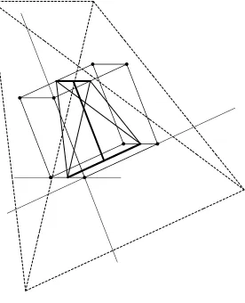
3The case n = 1 is very simple. For the segment S = [0,1], we have S =Q1. Therefore,ξ1 = 1and S is the unique perfect simplex. The equality
ξ1 = 1 could be also obtained from Theorem 3.
Consider the case n = 3. The conditions of Theorem 3 are satisfied, hence, ξ3 = 3. There exist a regular simplex S inscribed into Q3 such that
that α(S1) = P3i=1
Substituting vertices of Q3 into basic Lagrange polynomials we obtain
max
It follows from Theorem 1 and (24) that the extremal vertices of the cube, i. e., the vertices (1,1,1),(0,0,1),(0,1,0),(1,0,0)belong to the facets of the simplex 3S1. Every facet of 3S1 contains only one vertex of Q3. The rest
vertices of the cube belong to the interior of 3S1. Thus, though for S1 we
have S1 ⊂Q3 ⊂3S1, the simplex S1 is not perfect.
From (3), we obtain that three maximum segments in S1 parallel to
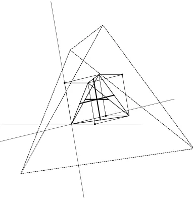
co-ordinate axes are intersected at the center of the cube. Now consider the simplex S2 with vertices 12,0,0
. For this simplex,
The formula (6) takes the form
ξ(S2) = 4 max
1≤k≤4 x∈maxver(Q3)
(−λk(x)) + 1.
Substituting vertices of Q3 into polynomials we obtain
−λ1(0,1,1) =−λ1(1,1,1) =−λ2(0,0,1) =−λ2(1,0,1) =
case all the vertices of Q3 are extremal. It follows from Theorem 1 and (25)
that each vertex of Q3 belongs to the boundary of3S2. Therefore,S2, unlike
S1, is a perfect simplex.
Bold lines mark the segments corresponding to the axial diameters.
6
The Exact Value of
ξ
5Theorem 4. There exist simplex S ⊂ Q5 such that simplex 5S is
circum-scribed around Q5 and boudary of 5S contains all vertices of the cube.
Proof. Consider the simplexS ⊂R5with vertices 1
2,1,
Matrices A and A−1 for the simplex S have the form
A=
polyno-mials for S are
It follows from (6) that
ξ(S) = 6 max that the simplex 5S is circumscribed around Q5. We get from (9) that each
axial diameter of S is equal to1. the condition (7) is satisfied. It has the form
max
This condition provides an alternative proof of the fact that simplex 5S is circumscribed around the cube Q5.
The list of vertices delivering the maximum in (26) includes all vertices of the cube. It means that (n−1)-dimensional faces of the simplex 5S (which form its boundary) contain all the vertices of the cube.
The theorem is proved.
Proof. LetS be the simplex from the proof of Theorem 4. Thenξ5≤ ξ(S) =
5. It follows from (11) that the inverse inequality ξ5 ≥ 5 holds. Therefore
ξ5 = 5.
It is easy to see that center of gravity ofS is the point 1 2, fact also can be obtained from Theorem 2.
The results of this section mean that there exist perfect simplices in R5. Moreover, we have found infinite family of such simplices. This family is described in the next section.
7
Some Family of Perfect Simplices in
R
5Consider the family of simplicesR =R(s, t)inR5with vertices s,1,1 R is nondegenerate and
Let us write down the basic Lagrange polynomials of R:
The axial diameters ofR can be found by (2):
d1(s, t) =d2(s, t) = 1,
Calculations with the use of (27) give
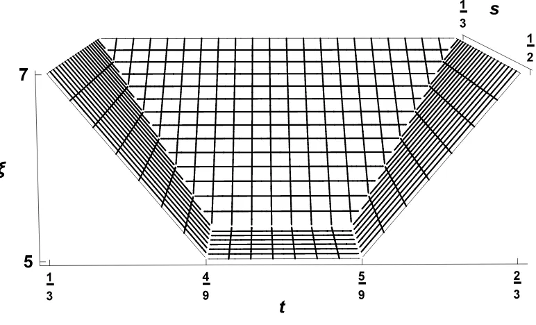
Figure 3: Graph of the functionξ =ξ(R(s, t))for s∈1
3, 1 2
, t∈1
3, 2 3
Applying (6), we obtain
ξ(R) = 6M(s, t) + 1 = 5, s∈4
9, 5 9
, t∈4
9, 5 9
;
ξ(R) = 6M(s, t) + 1>5, s /∈4
9, 5 9
, t /∈4
9, 5 9
. (30)
The graph of the function ξ = ξ(R(s, t)) for s ∈ 1
3, 1 2
, t ∈ 1
3, 2 3
is shown in Fig. 3. It follows from (30) and Collorary 6 that, if the conditions (28) are satisfied, then ξ(R(s, t)) =ξ5 = 5. Thus, R(s, t)⊂Q5 ⊂5R(s, t).
In the following we assume that (28) is true. Sinceξ(R) = 5 = dimR5, we haveα(R) =ξ(R)(see section 1). Therefore, the simplex5Ris circumscribed aroundQ5. The equalityα(R) = 5implies that axial diameters ofRare equal
to 1. If (28) holds true, then (29) takes the form
max
1≤k≤6 x∈maxver(Q5)
(−λk(x)) =
2
Table 1: Main extremal vertices
k Vertices ofQ5 such that(−λk(x)) =
2 3
for 4
9 ≤s≤ 5 9,
4
9 ≤t≤ 5 9
1 (0,0,0,0,0),(0,0,1,0,0), (1,0,0,0,0),(1,0,1,0,0)
2 (0,1,0,0,0),(0,1,1,0,0), (1,1,0,0,0),(1,1,1,0,0)
3 (0,0,0,1,0),(0,0,1,1,0),(0,1,0,1,0),(0,1,1,1,0),
(1,0,0,1,0),(1,0,1,1,0), (1,1,0,1,0),(1,1,1,1,0)
4 (0,0,1,0,1),(0,0,1,1,1),(0,1,1,0,1),(0,1,1,1,1),
(1,0,1,0,1),(1,0,1,1,1), (1,1,1,0,1),(1,1,1,1,1)
5 (1,0,0,0,1),(1,0,0,1,1), (1,1,0,0,1),(1,1,0,1,1)
6 (0,0,0,0,1),(0,0,0,1,1), (0,1,0,0,1),(0,1,0,1,1)
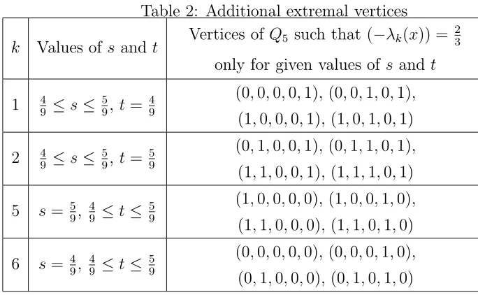
Table 2: Additional extremal vertices
k Values of s and t Vertices ofQ5 such that (−λk(x)) =
2 3
only for given values ofs and t
1 49 ≤s≤ 59, t= 49 (0,0,0,0,1), (0,0,1,0,1),
(1,0,0,0,1),(1,0,1,0,1)
2 49 ≤s≤ 59, t= 59 (0,1,0,0,1), (0,1,1,0,1),
(1,1,0,0,1),(1,1,1,0,1)
5 s= 59, 49 ≤t ≤ 59 (1,0,0,0,0), (1,0,0,1,0),
(1,1,0,0,0),(1,1,0,1,0)
6 s= 49, 49 ≤t ≤ 59 (0,0,0,0,0), (0,0,0,1,0),
The set of vertices of Q5 delivering maximum in (31), for given k, depends
on s and t. Let us study the behavior of the coefficients of basic Lagrange polynomials (27). If s and t satisfy (28), then 2 −3t > 0, 3t − 1 > 0,
3s−1 > 0, 2−3s > 0. For the rest of coefficients depending on s and t, we have inequalities 3t− 4
3 ≥ 0, 5
3 −3t ≥ 0, 3s− 5 3 ≤ 0,
4
3 −3s ≤0. These
expressions can be equal to 0 only on the boundary of the area (28). If the multiplier in front of xi is equal to0, thenxi does not influence the value of λk(x). Since, forx∈ver(Q5), the variablexi takes values0or1, the number of extremal vertices for λk(x) in this situation doubles.
The lists of vertices delivering maximum in (31) are given in Table 1 and Table 2. Denote Π =
(s, t) : 49 < s < 59, 49 < t < 59 . Using Theorem 1, we obtain the following result. For any (s, t) ∈ Π, the set ver(Q5) is divided
into 6 non-intersected classes of extremal vertices. Number of all extremal vertices is equal to 32, i. e., the number of vertices ofQ5. If(s, t)∈Π, then the
vertices of the same class are the inner points of the same 4-dimensional facet of the simplex 5R(s, t). The partition of ver(Q5) into classes is represented
in Table 1.
Additionally, ifk = 1,2,5,6, then, for some values of(s, t)(in particular, when (s, t)∈ ∂Π), some other vertices also will be extremal. All such cases are listed in Table 2. In each of these cases, corresponding vertices belong to two different 4-dimensional facets of 5R(s, t), i. e., belong to the facets of smaller dimension.
If one of s and t is the endpoint of 4
9, 5 9
, then the number of extremal vertices (considering repetitions) is equal to 36. If both s and t are the endpoints of the segment, then the number of extremal vertices (considering repetitions) is equal to 40.
It is easy to see that the center of gravity of R(s, t) coincides with the center of gravity of Q5. This fact could be also derived from Theorem 2.
8
Nonregular Extremal Simplices in
R
7Since 8 is an Hadamard number, it follows from Theorem 3 that there exist the regular simplex S ⊂Q7 such that ξ(S) =ξ7 = 7. In this section we
show that the property ξ(S) = ξ7 holds also for some nonregular simplices.
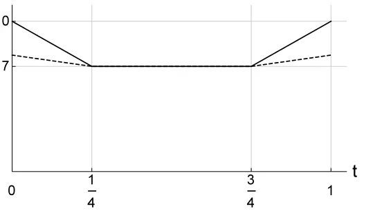
In this sense the case n= 7 is analogous to the case n = 3 (see section 5). LetT =T(t)be the simplex with vertices(1,0,0,0,0,0,1),(1,0,1, t,1,1,0),
(0,1,1,1−t,0,1,1), (0,0,0, t,1,1,0), (0,1,1,1−t,0,0,0), (1,1,0, t,1,1,0),
matrix A(t) for the simplex T has the form
Figure 4: The graphs of the functions α(T(t)) and ξ(T(t))
Consequently, for 1
4 ≤ t ≤ 3
4, we have α(T) = ξ(T) = 7. It means that
simplex 7T is circumscribed around Q7. The theorem is proved.
The graphs of the functionsα(T(t)) and ξ(T(t)) are shown in Fig. 4.
9
The Exact Value of
ξ
9In this section we show that ξ9 = 9. Moreover, we describe some family
of simplices S⊂Q9 such that ξ(S) = 9.
Let S = S(t) be the simplex with vertices (1,0,0,0,0,0,0,0,1),
(1,1,0,1, t,1,1,0,0), (1,0,1,1,1 − t,0,1,1,0), (0,1,1,1, t,0,0,1,1),
(0,1,1,0,1 − t,1,0,0,0), (0,0,0,1, t,0,1,1,0), (1,1,0,0,1 − t,1,1,1,0),
(0,1,1,0, t,1,1,0,1), (0,0,1,1,1 − t,1,0,1,1), (1,0,0,0,1,0,0,0,1).
If 0 ≤ t ≤ 1, then S(t) ⊂ Q9. Omitting the details, we present
charac-teristics of S:
det(A) = 25, vol(S) = |det(A)|
9! =
5
72576 = 0.00006889. . .
di(S) =
50
|10−25t|+|15−25t|+ 45, i6= 5; d5 = 1;
α(S) =
9, 2
5 ≤t≤ 3 5, 61
5 −8t, t < 2 5,
8t+215 , t > 35,
ξ(S) =
9, 2
5 ≤t ≤ 3 5,
25−40t, t < 25,
If 25 ≤t ≤ 35, then α(S) =ξ(S) = 9. Since ξ9 ≥ 9 (see (11)), we get ξ9 = 9.
It follows from the equality α(S) = ξ(S) that simplex 9S is circumscribed around Q9. Additional analysis shows that simplex S(t)is not perfect.
10
Concluding Remarks
The values α(S), ξ(S), di(S), ξn are connected with some geometric es-timates in polynomial interpolation. Detailed description of this connection can be found in the book [3]. These questions are beyond the scope of this paper.
Our results mean that, for all odd n from the interval 1 ≤n ≤ 9, holds ξn = n. This equality holds also for the infinite set of numbers n such that n+ 1 is an Hadamard number. We suppose that ξn = n for all odd n. However, by the time of submitting the paper, we have nor proof, nor refutation of this conjecture.
As it was mentioned above, perfect simplices in Rn exist at least for n = 1,3,5. It is unknown whether there exist perfect simplices for n > 5. It is also unclear whether there exist perfect simplices in Rn for any even n. Note that for n = 2 perfect simplices do not exist. This result follows from the full description of simplices S ⊂Q2 such that ξ(S) =ξ2, see [3].
The examples of extremal simplices for n = 5,7,9 were found partially with the use of computer. The families of simplices were constructed by generalization of individual examples. In particular, we utilized the property of simplices from Theorem 2. The figures were created with application of the system Wolfram Mathematica [9]. Despite the fact that we used numer-ical computations, all the results of this paper are exact and the proofs are complete.
References
[1] Nevskii, M. V. On a property of n-dimensional simplices. Mat. Zametki 87(4), 580–593 (2010) (in Russian). doi: 10.4213/mzm7698 English trans-lation: Nevskii, M. V. On a property of n-dimensional simplices. Math. Notes 87(3–4), 543–555 (2010) doi:10.1134/S0001434610030326
[3] Nevskii, M. V. Geometric estimates in polynomial interpolation. P. G. Demidov Yaroslavl State University, Yaroslavl (2012) (in Russian).
[4] Nevskii, M. V. Computation of the longest segment of a given direction in a simplex. Fundamentalnaya i prikladnaya matematica 18(2) 147–152 (2013) (in Russian). English translation: Nevskii, M. V. Computation of the longest segment of a given direction in a simplex. Journal of Mathe-matical Sciences 2013(6), 851–854 (2014) doi:10.1007/s10958-014-2175-6
[5] Nevskii M. V., Ukhalov A. Yu. On numerical characteristics of a simplex and their estimates. Modeling and Analysis of Information Systems 23(5), 603–619 (2016) (in Russian). doi:10.18255/1818-1015-2016-5-603-619
[6] Hall M., Jr. Combinatorial theory. Blaisdall publishing company, Waltham (Massachusets) – Toronto – London (1967)
[7] Hudelson M., Klee V., Larman D. Largest j-simplices in d-cubes: some relatives of the Hadamard maximum determinant problem. Linear Algebra Appl. 241–243, 519–598 (1996) doi:10.1016/0024-3795(95)00541-2
[8] Lassak M. Parallelotopes of maximum volume in a simplex. Discrete Com-put. Geom 21, 449–462 (1999) doi:10.1007/PL00009432
[9] Mangano S. Mathematica cookbook. O’Reilly Media Inc., Cambridge (2010)
[10] Nevskii M. Properties of axial diameters of a simplex. Discrete Comput. Geom 46(2), 301–312 (2011) doi:10.1007/s00454-011-9355-7
[11] Scott P. R. Lattices and convex sets in space. Quart. J. Math. Oxford (2) 36, 359–362 (1985)